Synthetic data generation for digital twins: enabling production systems analysis in the absence of data

ABSTRACT

Industry increasingly focuses on data-driven digital twins of production lines, especially for planning, controlling and optimising applications. However, the lack of open data on manufacturing systems presents a challenge to the development of new data-driven strategies. To fill this gap, the paper aim to introduce a strategy for generating random production lines and simulating their behaviour, thus enabling the generation of synthetic data. So far, such data can be recorded in event logs or machine status format, with the latter adopted for the use cases. To do so, the production lines are modelled using complex network concepts, with the system’s behaviour simulated via an algorithm in Python. Three use cases were assessed, in order to present possible applications. Firstly, the stabilisation of working, starved and blocked machines was investigated until a steady state was reached. The system behaviour was then investigated for different model parameters and simulation intervals. Finally, the production bottleneck behaviour (a phenomenon that can harm the production capacity of manufacturing systems) was statistically studied and described. The authors anticipate that this artificial and parametric data benchmark will enable the development of data-driven techniques without prior need for a real dataset.

KEYWORDS:

• Digital twins
• manufacturing systems
• data models
• complex systems
• simulation

1. Introduction

Recently, Industry 4.0 (I4.0) has influenced the development of new manufacturing execution systems (MESs), such as digital twins (DT) (Jaskó et al. 2020). A new era of smart manufacturing systems based on cyber-physical systems is disruptive to a variety of aspects of traditional manufacturing companies (Almada-Lobo 2015). In a highly digitalised, globalised and volatile disrupted environment, manufacturing companies are seeking to become more competitive (Mourtzis 2021). DTs may be considered an important tool in addressing this challenge, as they can precisely represent systems changes over time.

A DT is a virtual model, synchronised to a physical system through real-time data, thus allowing the simulation and analysis of performance, behaviour and potential outcomes (Segovia and Garcia-Alfaro 2022). The importance of DTs makes it essential to generate open datasets relating to manufacturing processes and to make them accessible to developers, researchers and students.

However, accessing manufacturing data is very difficult in the real world (Liu and Deng 2008). In other cases, shop floor sensors can be imprecise, representing 5–10% error levels (J. Li et al. 2009). This means the development of data-driven technologies is constrained by limited access to real databases within quality standards (Libes, Lechevalier, and Jain 2017). Accordingly, some authors regard the creation of representative benchmarks for processing data as one of the most important challenges in this research field (Aalst et al. 2011).

Data benchmarks consist of sample datasets and representative quality criteria for comparing tools and algorithms (Der Aalst Wil 2012b). These datasets can originate from different sources which come with associated pros and cons. The open datasets from real world processes TFIPM are available but do not usually describe production processes or have all the information anonymised. Another strategy for data generation is to use lab-scale physical models for data generation. This enables the development of essential technologies but requires a lot of human resources to implement (Lugaresi, Valerio Alba, and Matta 2021). Thus, using simulation in virtual environments is a promising way to make up for the lack of data access on production lines or in manufacturing systems (Libes, Lechevalier, and Jain 2017).

Simulation modelling is a popular technique for evaluating the design, operation and performance of complex systems (Friederich et al. 2022). It enables the modelling of current system behaviour and prediction of future behaviour in order to support decisions. However, these models are usually designed manually by simulation experts as it is a time-consuming task (Skoogh, Perera, and Johansson 2012). The present authors would argue that the time spent modelling these systems prevents developers, researchers and students from other fields (such as artificial intelligence, process mining and production systems, engineering) from generating their own data and scaling up their studies of digital twins. This gap constitutes the research problem that this paper aims to help to solve. Thus, the following question arises: ‘How can artificial manufacturing systems be generated and simulated at scale?’

To answer the research question, the authors set up three requirements to ensure the solution’s usability. Firstly, the data needs to match the digital twins’ data requirements, as detailed in sec:DT. Secondly, the process must be easy to run and user-friendly in a development environment. Finally, the strategy must be general enough to provide data representing not only the behaviour of a single system but of multiple systems with the same basic characteristics.

Consequently, the general objective of this paper is to develop a strategy to automatically generate production line layouts and simulate their behaviour. The authors’ vision is to generate useful data for digital twins and enable the testing, validation and prototyping of data-driven algorithms. This general objective is divided into five specific aims:

1. Conception of a flexible model for the generation of complex networks that can represent production systems in the most fundamental way; the Manufacturing Network Random Model (MN-RM);

2. Development of a throughput simulation system capable of performing the basic operating dynamics of a manufacturing system; the Complex Manufacturing Throughput Simulation (CLEMATIS);

3. Run an experimental use case with a huge number of systems: analyse the dynamic behaviour of the proposed network generation model under simulation;

4. Run a theoretical use case from the perspective of complex networks: study the underlying mechanisms affecting the state of the network; and,

5. Run a practical use case consisting of a probabilistic, experimental approach with practical applications: the Bottleneck Distribution Analysis.

To address the gap in benchmarking of manufacturing systems’ open datasets, a twofold strategy is proposed. Firstly, a network generation algorithm capable of generating randomised networks to represent a wide range of manufacturing systems. And secondly, a simulation strategy to simulate the networks that were generated. The most significant contribution of this research lies in the novel generation of manufacturing data. This can be a valuable resource for those lacking enough data to develop data-driven digital twins.

The remainder of this paper is organised as follows. Section 2.1 presents the theoretical background to digital twins and synthetic data generation. Section 3 describes the approach used to solve the first and second objectives (complex-network modelling and simulation system development). Section 4 summarises the findings of the designed model’s execution, characterisation and use cases; these are the third, fourth and fifth objectives. In Section 5 the results are presented and future research directions are proposed. Finally, Section 6 presents a summary of the paper’s achievements and research findings.

2. Literature review

A manufacturing process is defined as the use of one or more physical mechanisms to transform the shape or properties of a material (Chryssolouris 2006). Simply put, MES connects elements for sensing, decision-making and acting (Beregi et al. 2021). The MESs represented in a wide range of processes may be considered complex manufacturing networks (Zhan, Qingbo, and Tingxin 2014). In Industry 4.0, a smart manufacturing system (SMS) is a complex physical system that can be broken down into multiple digital models. This concept evolves simulation and modelling capabilities, interoperability, IoT sensors, tools and computing infrastructure (Leng et al. 2021).

The production system behaviours and properties can be recorded in event logs, or machine status or health monitoring databases (T. Li et al. 2017). These databases can be used to synchronise executable models and real systems (Friederich et al. 2022). The models in question are called digital twins. This context leads to an increased demand for large amounts of data (Cochran, Kinard, and Bi 2016).

When the digital twin concept is implemented, it becomes a system with a business life cycle. The key stages in a system’s life cycle are: concept, development, production, utilisation, support and retirement (Freund 2005). A digital twin relies on data synchronisation. Thus, it would require at least dummy data from its concept stage to understand what kind of analysis would be feasible and beneficial. However, collecting real data in all these stages is no trivial activity and requires a lot of resources.

Synthetic data generation is a useful and effective way of obtaining data. Some researchers fill this gap by generating data with lab-scale models or simulation models (Friederich et al. 2022; Libes, Lechevalier, and Jain 2017; Lugaresi, Valerio Alba, and Matta 2021). However, there is still a need for solutions to deal with specific system characteristics. The proposed alternative is to approach manufacturing systems as complex networks and use a graph generation strategy to enable system creation at scale. The following sections give a literature overview of the topics of digital twins data synchronization and synthetic data generation.

2.1. Digital twins data synchronisation

Industry is increasingly focused on digital shadows and twins of production lines, especially in planning, controlling and optimising applications (Shao 2021). Digital twins are suitably accurate and executable virtual models of physical things or systems (Wright and Davidson 2020). Similarly, shop floor operations can be described using simulation models. These are ranked among the top three tools for manufacturing system decision support (Skoogh, Johansson, and Stahre 2012). By integrating both concepts into a manufacturing system context, a simulation model may be used as the basic digital model for the development of a digital twin (Lugaresi and Matta 2018; Shao et al. 2019; Kumbhar, Ng, and; Buggineni 2023).

An entity-based reference model for this representation is presented in ISO 23,247–2:2021: Automation systems and integration – Digital twin framework for manufacturing (ISO 2020). Multiple different digital twins can be generated for one or more physical objects, based on the defined system requirements. The twinned object is used as a basis for creating a digital twin. In principle, the development of a digital twin based on a physical object could be data-driven or a manual process. The latter would be considered a kind of manual reverse engineering process (Tekinerdogan and Verdouw 2020).

The geometric, physical, behavioural and collaborative models are descriptive in nature, whereas the decision-making model is an intelligent, data-driven model (Semeraro et al. 2019). Thus, the digital twins are used to estimate the physical system’s response before it is triggered by an unexpected event (Schleich et al. 2017). The data that supports the modelling of smart factories may be categorised as state data, event data, or condition-monitoring data. All three are in a time-series format and thus each record consists of an observation and a timestamp (ts) (Friederich et al. 2021). The data categories are detailed below:

1. State data: records of the operational states of the system’s individual assets as working, starved, blocked and so on (Friederich et al. 2021);

2. Event data: records of event information generated by the system assets (timestamps, activity IDs and workpiece/order IDs) (Lugaresi and Matta 2021); and

3. Condition-monitoring data: records of relevant sensor data in time-series format (Friederich et al. 2022). In this paper, this category is regarded as a simply random seed that generates failures during the simulation.

It is possible to distinguish three levels of abstraction in the digital twin: (1) components, (2) systems and (3) systems of systems. In this context, components are bearings, systems are gearboxes and engines, while systems of systems are shop floors. Developing a digital twin requires the use of: (1) a physical entity, (2) a digital model of that entity, (3) a data extraction and communication protocol between the cyber and physical systems and (4) data analytics techniques (van Dinter, Tekinerdogan, and Raymon 2022). The data-driven and manual reverse engineering processes offer distinct advantages in developing digital twins for manufacturing systems.

Data-driven methods can yield cost-effectiveness by using existing data and reducing efforts during a development phase. While manual reverse engineering allows for more precise models, it requires more resources in the development phase. However, to select the appropriate process, it is necessary to consider such factors as the data availability and quality, desired level of detail, project timeline and budget constraints. In this paper, data is generated by the CLEMATIS simulation strategy, which represents the behaviour of the systems generated by MN-RM. This strategy can generate artificial dataset benchmarks from basic input parameters, with low computational costs and just a few input parameters.

2.2. Synthetic data generation

Real manufacturing data is not trivial to collect (Liu and Deng 2008), can present elevated error levels (J. Li et al. 2009) and access is often limited (Libes, Lechevalier, and Jain 2017). This situation constraints the development of new data-driven technologies for manufacturing, such as digital twins. In the research field of data-driven digital twins, some researchers filled this data gap with lab-scale representations (Friederich et al. 2022; Lugaresi, Valerio Alba, and Matta 2021) Also, simulations in virtual environments are a promising way of compensating for a lack of data (Libes, Lechevalier, and Jain 2017). But even so, building these representations can take huge effort and is a time-consuming task (Skoogh, Perera, and Johansson 2012).

The benefits of process modelling and simulating manufacturing systems is already well described in the literature (Brinksmeier et al. 2006; Tönshoff et al. 1992). For example, applying process simulations can reduce production time and costs (Mohan et al. 1998). Software such as FEDES (Finite Element Data Exchange System) uses simulated manufacturing process chains, including aeronautical engine components (Afazov 2013), to propose a methodology for sequentially simulating each step in a manufacturing process (Paralikas, Salonitis, and Chryssolouris 2013). Furthermore, the application of modelling and simulation techniques can assist with the decision-making during process planning (Rodrguez et al. 2015).

DT models are increasingly being used to improve the performance of complex manufacturing systems and can significantly enhance decision-making to mitigate the consequences of known bottlenecks (Latsou, Farsi, and Ahmet Erkoyuncu 2023). DT is based on data acquisition and processing and simulation plays a crucial role by enabling real-time communication. However, the complexity of industrial data poses some challenges (Stavropoulos and Mourtzis 2022). In the factory of the future, simulation may be a proven enabler throughout the manufacturing life cycle. Indeed, its integration with emerging technologies (in the form of digital twins) is one of the greatest challenges of the Fourth Industrial Revolution (Mourtzis 2020).

Although digital twins constitute a digital technology, various results validation steps (including expert insight) are required before deployment in a real-world environment (Mahesh, Ng, and Bandaru 2023). This means synthetic data is still valuable for various purposes (such as model validation, evaluation, data augmentation, input for artificial intelligence algorithms, and so on) (Chan, Rabaev, and Pratama 2022; Pires dos Santos et al. 2019; Smith and Dickinson 2022). For example, synthetic data and expert insights were used to validate DT models in high-risk, less digitised industries (Weerapura et al. 2023). This increased need for data occasioned several assessments. These addressed the issues and requirements surrounding the construction of synthetic data generators to provide data for scientists working in advanced manufacturing (Buggineni 2023; Libes, Lechevalier, and Jain 2017). However, none of the assessments found a strategy for generating parametric production lines and simulating data production at scale.

There has been an effort to generalise the understanding of manufacturing systems flexibility (Alexopoulos et al. 2007). Indeed, complex network techniques are suitable for dealing with the complicated relationships within production-line processes (Li et al. 2017a). The science of complex network arose from the necessity to understand the relationships between entities that traditional statistics and data analytics cannot handle (Wasserman and Faust 1994). Graph theory has also been widely applied to the modelling of real-world complex systems (Duchemin and De Castro 2023). However, due to the high dimensionality of graphs, it has been necessary to assume some structure to the data in order to extract useful information. Thus, random graph generation models were introduced to enable the study of specific network properties (Channarond 2015), such as the Erdös-Renyi model, scale-free networks (Barabási 2009), small-world networks (Watts and Strogatz 1998) and so on.

In the context of digital twins, data availability remains a significant challenge in contemporary scientific research. Balancing theoretical advancements with practical applications is crucial. Synthetic data offers a valuable solution by supporting theoretical understanding, model validation and automatic simulation model generation, plus other research domains. This perspective underscores the complementary role of real-world and synthetic data in driving progress and innovation within the field of digital twins. It allows research development without the limitations and consequences of a real-world application.

3. Methodology

In an effort to provide synthetic datasets for researchers and developers, the methodology is divided into two main functions. The first is the Manufacturing Network Random Model (MN-RM) which represents an algorithm for graph generation. These graphs are used as input to the Complex Manufacturing Throughput Simulation (CLEMATIS) script. The second function, CLEMATIS, is a complex network strategy for simulation. Thus, it become possible to generate databases from a series of initial parameters. Figure 1 shows how the methodology pipeline is organised.

Figure 1. Methodology pipeline from the user inputs to the use cases.

We argue that the statistical study of topological properties, node assignment strategy and system behaviour are the first steps in validating MN-RM and CLEMATIS strategies. Consequently, three basic characteristics are assessed in this paper: a) the system stabilisation, b) the impact of the failure rate on system function and c) the probabilistic distribution of bottleneck steps. To do this, the authors initially propose a continuous version of the CLEMATIS strategy that records machine state data. This simplification enables testing of the previous characteristics for long runs and an elevated number of machines or production steps.

The related code was structured using the Python programming language and igraph library (Csardi and Nepusz 2006) for the visual representation of graphs. All the libraries and programs are open source and free. The code used to implement this strategy is available in a GitHub repository.¹ The concepts necessary to understand the theory behind this implementation will be explained in the following subsections.

3.1. Random production line generator (MN-RM)

The MN-RM is presented as a solution for generating random production lines. To enable the study of the rich set of phenomena experienced in manufacturing systems, complex network concepts are applied to generate random systems. In this context, the production line can be represented as a graph network, with the machines being the nodes and directed edges representing the flow of materials in the process. The establishment of a fully connected network is achieved through a two-fold strategy. Each production step is initially assigned to a specific machine and then a random allocation of machines is carried out. This results in each machine being linked to all machines in the subsequent production step.

The proposed model generates networks based on two parameters: the total number of nodes (the total number of machines in the process), defined by $\mathit{n}$ and the number of production steps, defined by $\mathit{s}>0$. A production step is a point in the process with one or more identical machines and each machine performing exactly the same task: receiving raw materials in one state and transforming them in a subsequent state. Consequently, machines within the same production step are interchangeable and do not have edges between them.

The production steps are placed in ascending order, beginning with step 0 and ending with step $\mathit{s}-1$. Every node from production step $\mathit{i}$, where $0<\mathit{i}<\mathit{s}-1$, can receive materials from every node in the preceding production step $\mathit{i}-1$ and can supply materials for every node in the succeeding production step $\mathit{i}+1$. Hence, the nodes in step $\mathit{i}$ are fully connected with those in step $\mathit{i}-1$ and $\mathit{i}+1$.

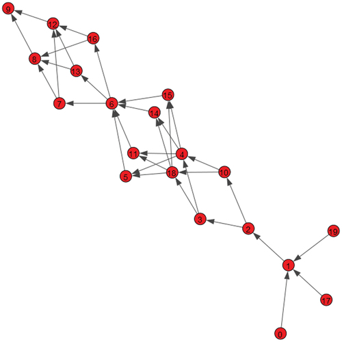
Moreover, for the network to be connected from start to finish, the number of nodes $\mathit{n}$ needs to be equal to, or greater than, the number of production steps $\mathit{s}$. If $\mathit{n}=\mathit{s}$, every production step will have a single node and the manufacturing process will be serial, with each machine feeding the next. On the other hand, if $\mathit{n}>\mathit{s}$, some production steps will have more than one node. In this case, the model generator will first place one node in each production step, to guarantee that no production step is disconnected. It will then place the remaining nodes randomly, following a uniform distribution. The Figure 2 shows an example of a network generated by the model.

Figure 2. Example of a production network with 20 nodes and 10 production steps.

Once the number of nodes and number of production steps have defined the whole topology of the network, the parameter alpha is calculated as

(1) $\mathit{\alpha }=\frac{s}{n},$(1)

To control their relationship. At least one node needs to be placed in each production step, so the number of nodes is always equal to or greater than the number of production steps. Consequently, $\mathit{\alpha }$ is in the interval $(0,1]$: values close to 0 being a production line with parallel nodes and 1 being one with serial nodes.

The algorithm will accept as input a number of machines greater than the number of production steps. The parameters are arbitrarily defined by the user and, once defined, are fixed throughout the simulation. All nodes share the same parameters. This paper focuses on analysing the topology of the network, so the effect of these parameter variations was not assessed. Thus, the only parameters affecting network structure are the number of steps and number of machines.

Other important parameters for the functioning of the networks are the production rate of the nodes, their failure rate and their buffer size. The production rate is the amount of material a node can output in a single iteration. The failure rate is the probability of a node failing in any given iteration (and encompassing all the real-world phenomena that might make a machine unavailable). Lastly, the buffer size is the maximum quantity of material a machine can have in its processing queue.

3.2. Virtual production line simulator (CLEMATIS)

This section aims to present, define and justify the CLEMATIS simulation strategy. According to Shannon (Shannon 1975) simulation is ‘the process of designing a model of a real system and conducting experiments with this model for the purpose either of understanding the behaviour of the system or of evaluating various strategies (within the limits imposed by a criterion or set of criteria) for the operation of the system’. Compared to other methods of production analysis, such as queuing theory or static capacity calculations, this tool mimics the dynamics of manufacturing systems and thus offers a great advantage (Skoogh, Johansson, and Stahre 2012).

There are different strategies for virtual simulation and they can be divided into numerical, script programming languages and commercial software with a graphical user interface. The numerical approaches are made using matrix or graph operations (a common strategy is the use of Petri Nets) (Villani 2004). Some examples are also available in (Haustermann, Wagner, and Moldt 2011). Regarding simulation using pre-built packages in scripting programming languages, the most common strategies are SimSharp for C#, SimJulia for Julia, Simmer for R and Simpy for Python (Lünsdorf and Scherfke 2002). Regarding software with a graphical user interface to allow detailed simulation of systems, the following can be highlighted: Rowkwel Arena (Lugaresi and Matta 2020), Visual Components, Enterprise Dynamics, Flexsim (Krenczyk 2014) and Siemens Tecnomatix Plant Simulation (Milde and Reinhart 2019).

These different simulation strategies have their pros and cons. While mathematical operations are much faster and have greater freedom, the complexity of the concepts can make their implementation harder. Although commercial software is much easier to understand, it is computationally heavier and usually offers constrained communication protocols with other platforms. Models based on pre-built scripts in open-source programming languages are an intermediate approach, lying between these previous two. Even so, there are still lower-level languages (C, C #) and higher-level ones suitable for data science applications (Julia, R, Python). In this context, the Python language and low-level mathematical implementation were chosen for their speed, ease of communication with other platforms and compatibility with statistical and process-mining packages. The purpose of this choice was to facilitate the first implementation’s passage through the barrier and make the work easier for subsequent users.

The main class of CLEMATIS is divided into two code blocks. The first creates the following arrays: production rates, buffers and states. It then organises the list of all system nodes according to their topology (production order) and creates the system time variable. From that, the second block is a for loop that goes through all productive nodes of each iteration. In these iterations, the state of the node is checked and, if the node is working, the entity in its buffer can be processed and delivered to the buffer of the next production step. The number of iterations is defined by the user at the beginning of the execution.

At this point, it is important to explain the three main data formats that can be recorded in a production line. The first is state data; this records the system’s operational states (working, turned off, starved or blocked) (Friederich et al. 2021). The second is the event log data; this records the start and end time of each activity, and can also include product identification and additional information (Lugaresi and Matta 2021). The third is the condition monitoring data; this records relevant health data from a system (Friederich et al. 2022). CLEMATIS can be used to generate event logs or state data. However, in this paper, the analysis used only state databases. This was done to allow the cases to exploit the most fundamental static and dynamic properties of the model. The data collection strategy will be explained in the next paragraph.

During production, the service principle is first-come first-served. Then, every node in the system can be in three states: starved, blocked and working. Firstly, a node is starved if its buffer is empty and consequently, it does not have any material to process. Secondly, a node is blocked if all its succeeding nodes have their buffers full and are unable to receive new materials. Finally, a node that has material in its buffer and can feed at least one node in the next production step is said to be working.

Furthermore, the nodes in the first production step are assumed to have an infinite quantity of raw materials available to them and thus they cannot be starved. Also, once nodes in the final production stage are completing products and not feeding any node in the network, there is no limit to their production capacity. Thus, they cannot be in the blocked state.

In each iteration of the production process simulation, the state of the nodes and quantity of material in their buffers is updated according to the topological order of the network. Additionally, in every iteration, a node that is working may experience failure according to the probability defined by its failure rate. The failure rate requires a seed to generate random failures in the system.

4. Use cases and model characterisation

This section presents three use cases demonstrating model capabilities and characterisation techniques. The aim is to study the dynamic behaviour of the proposed model and how well it represents what is found in real-world production systems. We anticipate the unlocking of potential for theoretical, practical and experimental studies for digital twins and production line performance evaluation.

Three use cases are presented. The first consists of the production simulation characterisation over random generated networks throughout a large number of iterations. It consists of an exploratory study of the network steady state, defined by the iteration number, following which the amount of starved, blocked and working nodes do not vary over time.

The second use case seeks to understand how the topology of the network affects its dynamic behaviour under simulation. Doing this means observing the distribution of working node changes with $\mathit{\alpha }$. These results are then interpreted from the perspective of the Theory of Constraints (TOC), which defines a production bottleneck as ‘any resource whose capacity is equal to or less than the demand placed upon it’ (Goldratt and Cox 2016). In this case, this means the production bottleneck step is the one with fewer machines working.

The third use case relies on the TOC concepts that (i) every system has a constraint and (ii) that this constraint is an opportunity for improvement (Rahman 1998). The TOC working principle is known as the Process of Ongoing Improvement (POOGI) and the first POOGI step is always to identify a system’s bottleneck (Wu, Zheng, and Shen 2020). Assuming this to be important, the purpose of this use case is to develop an analytical formulation of the probabilistic distribution of machines in the bottleneck step. The analytical results are then compared to the experimental results in order to validate the approach.

In the analyses, only the system’s asymptotic properties are considered. This means considering the state of the system after many iterations, when a proportion of the nodes in each state has already converged. The simulations are also repeated many times, with only the average node properties of each state being analysed. This means that specific instances of system state are not considered. Thus, as the number of iterations increases, the choice of a specific seed does not change the asymptotic results.

The authors anticipate that these use cases will enable a basic understanding of how the framework can be executed and analysed. When the digital twin concepts are implemented, this analysis may be executed, results compared and digital twin models validated. This comparison can be run as a model-based validation, properties test (Hua, Lazarova-Molnar, and Francis 2022) or time-series analysis (Lugaresi et al. 2022).

4.1. Use case 1: experimental stability analysis

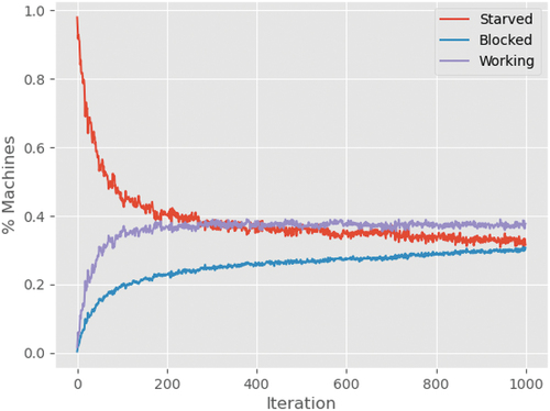
First, it is analysed how the distributions of nodes in the working, starved and blocked states change over time and whether the networks that are generated reach a steady state. We produced 30 samples of the network and ran each sample through 1000 iterations, observing for each iteration the percentage of nodes in each state. The simulated networks have $\mathit{\alpha }=0.5$, with $\mathit{n}=500$ machines distributed in $\mathit{s}=250$ production steps. The production rate and buffer size are unitary and the failure rate is 0.1.

The results are shown in Figure 3. It may be observed that all nodes start in the starved state, as no material has been produced yet and so the node buffers are empty. As the iterations progress, the fractions of nodes in the working and blocked states grow until they reach a steady state. For the working nodes, it is visible that after iteration 400 their quantities remain stable, comprising fewer than 40% of all the nodes in the network. This behaviour shows that the networks have found stability, are able to leave the transient state and reach a steady state.

Figure 3. Percentage of nodes in the starved, blocked and working states with respect to the number of iterations.

In practice, this state represents the stabilisation of a production line when productivity is constant. In this experiment, it is possible to understand this initial stage of production in large production lines. Furthermore, in future experiments, it might be possible to set a finite number of entities to be processed and then analyse the behaviour of the production line until its complete stop. This type of experiment may also be used as a basis for studying batch production or production stage scheduling.

4.2. Use case 2: complex network behaviour and topology

Once we have evidence that the system is stable, starts the investigation (in the steady state) on how the distribution of working nodes is affected by the network topology, as described by the parameter $\mathit{\alpha }$. The experiments vary $\mathit{\alpha }$ starting from 0.025, indicating a network with most nodes in parallel and increasing its value until reach 1.0, a network with all nodes in series. This analysis should help us understand the role of the production network topology in the overall efficiency of the system, as inferred from the percentage of working nodes.

We generate networks with $\mathit{n}=500$ nodes, varying the number of production steps in the range $\mathit{s}\in [25,500]$, for networks with failure rates of 0.0 and 0.1. All networks have production rates and buffer sizes of 1.0. 25 samples are generated for each configuration.

The results can be seen in Figure 4. It is possible to observe the same behaviour in both curves, represented by an asymmetrical V-shaped graph. When $\mathit{\alpha }$ is almost zero and the networks are close to becoming totally parallel, the percentage of working nodes is relatively high. As $\mathit{\alpha }$ increases and the networks become more serialised, the percentage of working nodes decreases at a rapid pace, reaching a minimum when $\mathit{\alpha }$ is close to 0.2. After that, the percentage of working nodes starts increasing again, until it reaches the point where the network is totally serial, when $\mathit{\alpha }=1.0$.

Figure 4. Percentage of working nodes with respect to $\mathit{\alpha }$.

This behaviour indicates that our system is experiencing a phase transition, in which its working regime changes. In the first working regime, that goes from roughly $\mathit{\alpha }=0$ to $\mathit{\alpha }=0.2$. The smaller the $\mathit{\alpha }$ value, the higher the percentage of working machines. When $\mathit{\alpha }$ values are closer to 0.2, it is possible to see the lower ratios of working machines. However, once the point at which $\mathit{\alpha }=0.2$, (which is called ${\alpha }_{\mathit{critical}}$), the system shows the opposite behaviour; the more serial it is, the more efficient it gets. This is an interesting result which may have useful implications for real-life production systems.

To interpret why the network experiences two working regimes for different ranges of $\mathit{\alpha }$, two important characteristics of the simulation model are highlighted. Firstly, it assumes the first production step in the network has an infinite quantity of raw materials available to it and thus cannot be starved. Secondly, it assumes that the last production step in the network has no restrictions on how much it can produce and thus cannot be blocked.

With these two conditions, the authors argue that when $\mathit{\alpha }\to 0$ and our network topology is a single production step with a large number of nodes, the % working value goes to 100%. This conclusion stems from the fact that if the network has only one production step, then this is simultaneously both the first and the last production step. Thus, the only possible state for its nodes is working. This situation is illustrated in Figure 5a.

Figure 5. (a) Totally parallel production network, $\mathit{\alpha }=0.0$. (b) Totally serial production network, $\mathit{\alpha }=1.0$.

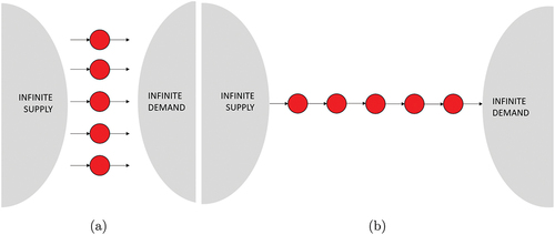
At the other extreme of the spectrum, when $\mathit{\alpha }=1.0$, the number of nodes is equal to the number of production steps. Consequently, every production step will have a single node and the network will be totally serial, similar to a linked list. This scenario is illustrated in Figure 5b. Furthermore, in the situation where all nodes have a failure rate equal to zero and all nodes have the same production rate of one, consequently the materials produced at the first node will flow to the last one uninterrupted. No node will ever be starved or blocked. This is consistent with the results of the experiment illustrated in Figure 4.

We thus conclude that, if our failure rate is equal to zero for both $\mathit{\alpha }=0$ and $\mathit{\alpha }=1$, all nodes in the network will be working in steady space. In order to explain the behaviour of the intermediate values of $\mathit{\alpha }$, the concept of a production bottleneck is introduced. This the point in the process with the minimum productivity, or minimum production rate. It restricts the production of the whole process and, if its productivity increases, the overall productivity of the system will also increase.

For our network, the production capacity of each production step is the sum of the production rates of the nodes present in that production step. Assuming the production rate to be unitary for every node, the capacity of a production step is the number of nodes in that production step. Consequently, the bottleneck in our network is the production step with the smallest number of nodes. This step will be called bottleneck step and it is illustrated in Figure 7.

Figure 6. Production network with 20 nodes and 8 production steps. Every node has a production rate of 1.0, so the production capacity in a production step is the sum of nodes in it. The bottleneck step is the production step with the smallest production capacity of the network.

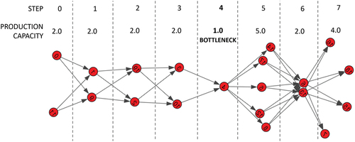
From this definition, it is possible to observe that all the production steps may have a maximum number of working nodes, which is equal to the number of nodes in the bottleneck step. If a production step comes before the bottleneck step and has more nodes than the bottleneck, then the excess nodes will be blocked because the bottleneck does not have enough capacity. For instance, production step 3 in Figure 6 has a production capacity of 2.0, while the bottleneck has a production capacity of only 1.0. Consequently, production step 3 will always have one node blocked in the steady state. Similarly, if a production step comes after the bottleneck step and has more nodes than the bottleneck, the excess nodes will be starved. For example, the production step 5 in Figure 6 has a production capacity of 5.0 but the bottleneck can provide it with a production of only 1.0, so it will have 4 starved nodes in the steady state.

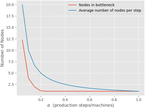
Knowing that the nodes are placed randomly in the network following a uniform distribution the network grows beyond a single production step, and a bottleneck will always be present. To further investigate this point, it was registered (for networks with $\mathit{\alpha }$ in the range $(0,1.0]$) the number of nodes in the bottleneck step and the average number of nodes per step. The curves are shown in Figure 7. For all values of $\mathit{\alpha }$, except $\mathit{\alpha }=1.0$, there is a bottleneck step. In other words, the average number of nodes in a production step is greater than the number of nodes in the bottleneck. Furthermore, it can be seen that the difference between the average number of nodes in a production step and the number of nodes in the bottleneck step decreases as $\mathit{\alpha }$ grows. This difference indicates the average number of idle nodes per step. This number is greater for networks with smaller values of $\mathit{\alpha }$. The definition of idle nodes comprises all nodes that are not working.

Figure 7. Average number of nodes per production step and number of nodes in the bottleneck step with respect to $\mathit{\alpha }$.

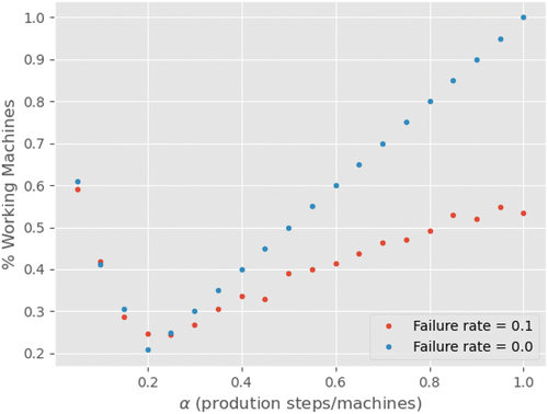
We can calculate the total number of idle nodes in the network by multiplying the average number of idle nodes per step by the total number of steps in the network. After normalising this value, the percentage of working nodes is found by simply reducing it by one. The curve obtained this way is shown in Figure 8, plus the curve obtained by simulating the networks with a failure rate equal to zero.

Figure 8. Percentage of working nodes with respect to $\mathit{\alpha }$, obtained using bottleneck analysis and experimentally through simulation.

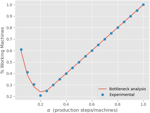
We can see that both curves agree almost perfectly. This shows that our reasoning as to the mechanism that determines whether a node is working or not in the steady state is correct. Even more importantly, bottleneck analysis (as developed here) is an important discipline for production engineers and is relevant for understanding the production capacity of real-world manufacturing systems. Our model can successfully simulate the fundamental behaviours of such systems.

4.3. Use case 3: bottleneck distribution analysis

In this section, it is presented an hybrid use case comparing the theoretical, probabilistic distribution of bottlenecks and the experimental results observed. Our objective is to parameterise the number of machines in the bottleneck stage, according to the model input variables. The analysis is divided into two stages. The first describes the analytical approach to developing probabilistic distribution equations, while the second presents the experimental results of implementing the model.

A summary of the first stage will be presented below. The process of assigning machines to production steps was first modelled as a random allocation, similar to the balls and bins problem (Mitzenmacher, Richa, and Sitaraman 2001). However, the complex characteristics of the minimum anticipated value distribution of the number of machines in each production step (Leadbetter, Lindgren, and Rootzén 2012) led to the use of a simplified approach to this problem. The upper limit of the lower tail of the Poisson cumulative distribution function is used as the number of machines assigned to the bottleneck step, with a probability equal to $\frac{1}{s}$.

The second stage presents the experimental results of this approach. Thus, simplification could be seen to yield satisfactory results. It became clear that there is a critical alpha, in which the number of machines assigned to the bottleneck step becomes null or equal to one (in the case of CLEMATIS).

To initiate the first stage, it is necessary to declare the statistical variables of the problem. Thus, let $X_i$ be the number of machines randomly assigned to step $\mathit{i}=0,\dots ,\mathit{s}-1$ such that:

(2) $\sum _{\mathit{i}=0}^{\mathit{s}-1}{X}_i=\mathit{n}.$(2)

Each network/production line can be constructed given a fixed $\mathit{\alpha }=\frac{s}{n}$, that represents the inverse of the Poisson rate parameter $\mathit{\lambda }=\frac{1}{\alpha }$. The authors also assume independence between the variables representing the number of machines assigned to each step, $X_i\mathrm{\perp }{X}_j,\mathrm{\forall }\mathit{i}\ne \mathit{j}$ and that $X_i\sim \mathrm{Poisson}(\mathit{\lambda })$ for $\mathrm{\forall i}$. Hence, the probability mass function is given by:

(3) $\mathit{P}(\mathit{X}=\mathit{k})=\frac{{\lambda }^k{e}^{-\mathit{\lambda }}}{\mathit{k}!},$(3)

and the cumulative distribution function is:

(4) $\mathit{P}(\mathit{x}\le \mathit{k})=\left\{\begin{array}{c}0,\mathrm{if}\mathit{x}\le 0,\\ e^{\lambda }{\sum }_{i=0}^k\frac{{\lambda }^i}{\mathit{i}!},\mathrm{otherwise}.\end{array}\right.$(4)

We want to estimate $\mathit{Y}$, that is the number of machines located in the bottleneck step, where:

(5) $\mathit{Y}=\mathit{min}(X_0,X_2,\dots ,X_{\mathit{s}-1}).$(5)

This equation is studied in the field called ‘extreme value distribution theory’ (Leadbetter, Lindgren, and Rootzén 2012) and can be rewritten as:

(6) $\mathit{Y}=-\mathit{max}(-X_0,-X_2,\dots ,-X_{\mathit{s}-1}).$(6)

At this point, it is important to note that the phenomenon is studied from the perspective of the distribution of attempts to assign machines to each step. This machine assignment process is described by a uniform probability distribution in the production steps, which leads us to assume the following relationship:

(7) $\mathit{P}(X_i\le \mathit{Y})=\frac{1}{s}.$(7)

Thus, this relationship is assumed to represent the first quantile of the Poisson cumulative distribution function, which is related to the number of machines in the bottleneck step. Then, considering the R-th quantile equation of Y for R $\in (0,1)$ (Short 2013), obtained from the Poisson distribution:

(8) $\mathit{Q}(\mathit{\lambda },\mathit{R})=\min \mathit{k}\in \mathcal{N}\mathrm{such}\mathrm{that}\mathit{P}(\mathit{Y}\le \mathit{k})\ge \mathit{R}.$(8)

Consequently, considering $\mathit{R}=\frac{1}{s}$ it is possible to rewrite the quantile function as:

(9) $\mathit{Q}(\mathit{\lambda },s^{-1})=\min \mathit{k}\in \mathcal{N}\mathrm{such}\mathrm{that}\mathit{P}(\mathit{Y}\le \mathit{k})\ge s^{-1}$(9)

Finally, the objective becomes finding the value of $\mathit{k}$, which will be admitted and evaluated as equivalent to Y. This value can be found by the inverse of the survival function (Fs) (Virtanen et al. 2020) – considering $\mathrm{Fs}(\mathit{k},\mathit{\lambda })=1-\mathrm{CDF}(\mathit{k},\mathit{\lambda })$, where CDF is the cumulative density function of the Poisson distribution:

(10) $\mathit{P}(X_i\le \mathit{k};\mathit{\lambda })=\mathrm{CDF}(\mathit{k},\mathit{\lambda }).$(10)

and, by substitution, letting $\mathit{k}=\mathit{Y}$:

(11) $s^{-1}=1-\mathrm{Fs}(\mathit{Y},\frac{n}{s})$(11)

which leads us to the inverse survival function that will be applied to estimate the value of $\mathit{Y}$:

(12) $\mathit{Y}=\mathrm{F}{\mathrm{s}}^{-1}(1-s^{-1},\frac{n}{s}).$(12)

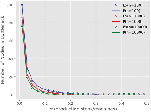
An experiment was designed to validate the analytical results obtained through this quantile approach. For this experiment, each production network was built 50 times with 100, 1,000 and 10,000 nodes, varying the alpha values from 0.01 to 0.5, in steps of 0.02. The number of machines present in the bottleneck step of each network was then observed. Using the quantile approach, the average number of machines in the bottleneck step over the 50 repetitions of each production network composition was compared with the analytical values obtained.

The results are presented in Figure 9, in which is visible the decay of the number of nodes in the bottleneck step proportional to the alpha growth, or lambda decay. Moreover, the analytical result was close to the average throughout all the experiments that were conducted. It was therefore possible to model the machine distribution problem in the bottleneck stage using the same parameters as for the MN-RM and CLEMATIS model.

Figure 9. Number of machines in the bottleneck step, obtained using the statistical model and experimentally through simulation.

5. Discussions and future research directions

There is a lack of research into evolution laws and performance evaluation for manufacturing networks (Li et al. 2017a). The parameterised probabilistic behaviour of MN-RM strategy was assessed in order to provide some examples of practical analysis. The minimum number of nodes assigned to a step was demonstrated analytically. The authors would argue that these analyses can be conducted with a wide variety of input parameter indicators. Hence, MN-RM can be used as a basis for statistical, probabilistic and multivariate analyses (Curry and Feldman 2010; Pansare, Yadav, and Nagare 2023). Furthermore, this generative model was developed using concepts from the research area of complex networks (Cohen and Havlin 2010). This allows analysis of these production line mechanisms from the perspective of complex networks (Becker, Meyer, and Windt 2014; Li et al. 2017b).

To understand how the manufacturing system behaves for different topological characteristics, the variable $\mathit{\alpha }$ was defined to control the network seriality. This means that $\mathit{\alpha }\to 0$ represents a totally parallel network and $\mathit{\alpha }=1.0$ a totally serial network. These process architectures may be defined by different nomenclatures in the bibliography, an example being the Lasagna or Spaghetti Processes (Van der Aalst 2011).

A subsequent step in this study was the development of CLEMATIS, a module that provides network simulation and data generation capabilities. By executing this module, machine state data and event logs can be generated. The strategy was implemented from scratch and followed the anticipated behaviour, as demonstrated by stability analysis. In the steady state, it was possible to observe the following phenomenon: the percentage of working nodes starts relatively high, for small values of $\mathit{\alpha }$ and decreases until it reaches a critical value. At this point, the system undergoes a phase transition, changing its working regime. For values of $\mathit{\alpha }$ greater than the critical value, the percentage of working nodes increases until $\mathit{\alpha }$ reaches 1.0.

It is important to emphasise that this strategy is still in fundamental form. Thus, future research directions include three main pathways that are synchronised with the methodology pipeline, as shown in Figure 10. Each of the proposed objectives for this paper is linked to a particular future research direction. From the model input parameters to the use cases, there are opportunities that will be explained in this section.

Figure 10. Future Research directions synchronised with the methodological pipeline.

Firstly, improvement measures for the model implementation. These include the capability to input unbalanced parameters, implement a simulation strategy based on more libraries and improve user capabilities. This solution can promote more realistic behaviours, of the kind likely to be faced in production environments. To summarise, heterogeneous failure rates, production rates and buffer sizes can be implemented in order to exploit the model under harsher conditions. Synthetic data helps simulate various ‘what-if’ scenarios, thus aiding assessment of the impact of parameter changes on production line performance without costly real-world adjustments. Finally, synthetic data supports training and education by offering a safe environment for personnel to learn about manufacturing system behaviour and operations.

Secondly, implementing strategies for production line performance evaluation using these datasets as benchmark. There are three promising future research directions: (I) processing the data through artificial intelligence and machine learning for data-driven analysis, such as studying bottlenecks in production systems (Subramaniyan et al. 2020, 2021). (II) simulation-based optimisation techniques (Swisher, Jacobson, and Yücesan 2003), such as ensuring the process of ongoing improvement in production lines (Wu, Zheng, and Shen 2020). (III) these artificial databases can be used as benchmarks for process mining techniques (Der Aalst Wil 2012a; der Aalst et al. 2003; der Aalst, Wil, and Maruster 2004; Van der Aalst 2011).

Thirdly, use this strategy as an input for the development, evaluation and validation of digital twins in a safe environment, as the data requirements are the same as those presented in 2.1. This model may be built according to the reference framework for manufacturing digital twins presented in ISO 23,247–1 (ISO 2020). Optimising production planning, scheduling and routing problems are among the main applications for digital twins. Thus, these artificial databases enable implementations for resource (such as materials labour and equipment) optimisation, cycle-time reduction and inventory cost reductions (Shao and Helu 2020).

6. Conclusions

In the introduction, three solution requirements were set up and the authors argued that the requirements were satisfied. Firstly, the MN-RM strategy can generate a wide variety of production systems (represented by complex networks) and simulate them simply by using CLEMATIS. Secondly, this approach is easy to run and can be imported from GitHub and executed locally at low computational cost. The only requirement is that Python is installed on the computer device. Thirdly, the three use cases demonstrate how the analysis may be made at scale, by varying the input parameters.

In order to represent the production lines simply, the data generated needs to fit the digital twin requirements explained in 2.1. The authors propose a solution consisting of a two-step approach that can generate manufacturing systems and simulate them. The asymptotic behaviour of status machine data is studied. The first step is called MN-RM, a strategy that assigns a defined number of machines to a defined number of production steps according to a Poisson probability distribution. The second step is called CLEMATIS, a simulation strategy that represents the production in the production lines that were built in the previous step. The input parameters are the number of production steps, the number of machines and the number of products to be processed. After running the codes, the output can be an event log or a machine status database.

We observed that our proposed model allows the construction of a set of statistically parameterised complex layouts. Thus, it is possible to simulate these layouts and generate data to analyse their static and dynamic properties. There is evidence that the proposed simulation is stable. This means that for a large number of iterations, the quantity of nodes in each state becomes constant, reaching a steady state. The experiments demonstrated that this behaviour can be explained using the very well-known concept of bottleneck analysis, which is often used to understand the productivity of real-world systems. This concept was validated by reproducing the results from the simulation using an analytical probabilistic approach. This is a good indication of our model’s ability to reproduce the behaviour of real manufacturing systems.

The data generated from CLEMATIS and MN-RM plays a pivotal role in digital twin application enhancement. Firstly, it can facilitate model calibration and validation by comparing simulated data with real-world data, ensuring that digital twin models faithfully represent physical manufacturing systems. Secondly, it enables predictive analysis through machine-learning training, supporting proactive decision-making and optimisation. Thirdly, it can be used for simplified real-time performance monitoring, where digital twins continuously align their simulated behaviour with live synthetic data for validation purposes. Fourthly, synthetic data aids in simulating various ‘what-if’ scenarios and helps assess the impact of parameter changes on production line performance without costly real-world adjustments. Finally, synthetic data supports training and education by offering a safe environment for personnel to learn about manufacturing system behaviour and operations. The authors argue that this foundational dataset generation strategy is indispensable for digital twins advancements, enabling them to faithfully mimic the system’s behaviour and performance in a safe and flexible environment.

Disclosure statement

No potential conflict of interest was reported by the author(s).

Additional information

Funding

This work was supported by the Coordenação de Aperfeiçoamento de Pessoal de Nível Superior.

Notes

1. https://github.com/Victorf-lopes/clematis.git.

References

- Aalst, W. V. D., A. Adriansyah, A. K. A. de Medeiros, F. Arcieri, T. Baier, T. Blickle, J. Chandra Bose, et al. 2011. “Process Mining Manifesto.” In Business Process Management Workshops: BPM 2011 International Workshops, 169–194. Clermont- Ferrand, France: Springer Berlin Heidelberg, August 29.
- Afazov, S. M. 2013. “Modelling and Simulation of Manufacturing Process Chains.” CIRP Journal of Manufacturing Science and Technology 6 (1): 70–77. https://doi.org/10.1016/j.cirpj.2012.10.005.
- Alexopoulos, K., N. Papakostas, D. Mourtzis, P. Gogos, and G. Chryssolouris. 2007. “Quantifying the Flexibility of a Manufacturing System by Applying the Transfer Function.” International Journal of Computer Integrated Manufacturing 20 (6): 538–547. https://doi.org/10.1080/09511920600930046.
- Almada-Lobo, F. 2015. “The Industry 4.0 Revolution and the Future of Manufacturing Execution Systems (MES).” Journal of Innovation Management 3 (4): 16–21. https://doi.org/10.24840/2183-0606_003.004_0003.
- Barabási, A.-L. 2009. “Scale-Free Networks: A Decade and Beyond.” Science 325 (5939): 412–413. https://doi.org/10.1126/science.1173299.
- Becker, T., M. Meyer, and K. Windt. 2014. “A Manufacturing Systems Network Model for the Evaluation of Complex Manufacturing Systems.” International Journal of Productivity and Performance Management 63 (3): 324–340. https://doi.org/10.1108/IJPPM-03-2013-0047.
- Beregi, R., G. Pedone, B. Háy, and J. Váncza. 2021. “Manufacturing Execution System Integration Through the Standardization of a Common Service Model for Cyber-Physical Production Systems.” Applied Sciences 11 (16): 7581. https://doi.org/10.3390/app11167581.
- Brinksmeier, E., J. C. Aurich, C. H. Edvard Govekar, H.-W. Hoffmeister, F. Klocke, J. Peters, et al. 2006. “Advances in Modeling and Simulation of Grinding Processes.” CIRP Annals 55 (2): 667–696. https://doi.org/10.1016/j.cirp.2006.10.003.
- Buggineni, V. 2023. “Utilizing Synthetic Data Generation Techniques to Improve the Availability of Data in Discrete Manufacturing for AI Applications: A Review and Framework.” Order No. 30315940. University of Georgia ProQuest Dissertations Publishing. Available from ProQuest Dissertations & Theses Global: The Sciences and Engineering Collection. 2823787457. http://proxy.lib.chalmers.se/login?url=https://www.proquest.com/dissertations-theses/utilizing-synthetic-data-generation-techniques/docview/2823787457/se-2.
- Channarond, A. 2015. “Random Graph Models: An Overview of Modeling Approaches.” Journal de la Société Française de Statistique 156 (3): 56–94.
- Chan, K. C., M. Rabaev, and H. Pratama. 2022. “Generation of Synthetic Manufacturing Datasets for Machine Learning Using Discrete-Event Simulation.” Production & Manufacturing Research 10 (1): 337–353. https://doi.org/10.1080/21693277.2022.2086642.
- Chryssolouris, G. 2006. Manufacturing Systems: Theory and Practice. 2nd ed. New York: Springer-Verlag.
- Cochran, D. S., D. Kinard, and Z. Bi. 2016. “Manufacturing System Design Meets Big Data Analytics for Continuous Improvement.” Procedia CIRP 50:647–652. https://doi.org/10.1016/j.procir.2016.05.004.
- Cohen, R., and S. Havlin. 2010. Complex Networks: Structure, Robustness and Function. New York, USA. Cambridge University Press.
- Csardi, G., and T. Nepusz. 2006. “The Igraph Software Package for Complex Network Research.” InterJournal Complex Systems 1695. https://igraph.org.
- Curry, G. L., and R. M. Feldman. 2010. Manufacturing Systems Modeling and Analysis. Verlag GmbH, Berlin: Springer Science & Business Media. https://doi.org/10.1007/978-3-642-16618-1.
- Der Aalst Wil, V. 2012a. “Process Mining.” Communications of the ACM 55 (8): 76–83. https://doi.org/10.1145/2240236.2240257.
- Der Aalst Wil, V. 2012b. “Process Mining: Overview and Opportunities.” ACM Transactions on Management Information Systems 3 (2): 1–17. https://doi.org/10.1145/2229156.2229157.
- der Aalst, V., T. W. Wil, and L. Maruster. 2004. “Workflow Mining: Discovering Process Models from Event Logs.” IEEE Transactions on Knowledge and Data Engineering 16 (9): 1128–1142. https://doi.org/10.1109/TKDE.2004.47.
- der Aalst, V., M. P. Wil, B. F. Van Dongen, J. Herbst, L. Maruster, G. Schimm, and A. J. Weijters. 2003. “Workflow Mining: A Survey of Issues and Approaches.” Data & Knowledge Engineering 47 (2): 237–267. https://doi.org/10.1016/S0169-023X(03)00066-1.
- Duchemin, Q., Y. De Castro, R. Adamczak, N. Gozlan, K. Lounici, and M. Madiman. 2023. “Random Geometric Graph: Some Recent Developments and Perspectives.” High Dimensional Probability IX: The Ethereal Volume 80 347–392. https://doi.org/10.1007/978-3-031-26979-0_14.
- Freund, E. 2005. “ISO/IEC 15288: 2002, Systems Engineering-System Life-Cycle Processes.” Software Quality Professional 8 (1): 42.
- Friederich, J., S. Chung Jepsen, S. Lazarova-Molnar, and T. Worm. 2021. ” “Requirements for Data-Driven Reliability Modeling and Simulation of Smart Manufacturing Systems.” In 2021 Winter Simulation Conference (WSC), edited by S. Kim, B. Feng, K. Smith, S. Masoud, and Z. Zheng, 1–12. Phoenix, AZ, USA: IEEE. https://doi.org/10.1109/WSC52266.2021.9715410.
- Friederich, J., D. P. Francis, S. Lazarova-Molnar, and N. Mohamed. 2022. “A Framework for Data-Driven Digital Twins for Smart Manufacturing.” Computers in Industry 136:103586. https://doi.org/10.1016/j.compind.2021.103586.
- Goldratt, E. M., and J. Cox. 2016. The Goal: A Process of Ongoing Improvement. Abingdon, UK: Routledge.
- Haustermann, M., T. Wagner, and D. Moldt. 2011. “Petri Nets Tools Database Quick Overview.” Accessed November 16, 2022. https://www2.informatik.uni-hamburg.de/TGI/PetriNets/tools/quick.html.
- Hua, E. Y., S. Lazarova-Molnar, and D. P. Francis. 2022. ”Validation of Digital Twins: Challenges and Opportunities.” In 2022 Winter Simulation Conference (WSC), Singapore, edited by F. Ben, P. Yijie, G. Pedrieli, S. Eunhye, S. Shashaani, and C. Corlu, 2900–2911. New York City, USA: IEEE.
- ISO. 2020. DIS 23247-1 Automation Systems and Integration—Digital Twin Framework for Manufacturing. Geneva, Switzerland: International Organization for Standardization.
- Jaskó, S., A. Skrop, T. Holczinger, T. Chován, and J. Abonyi. 2020. “Development of Manufacturing Execution Systems in Accordance with Industry 4.0 Requirements: A Review of Standard-And Ontology-Based Methodologies and Tools.” Computers in Industry 123:103300. https://doi.org/10.1016/j.compind.2020.103300.
- Krenczyk, D. 2014. “Automatic Generation Method of Simulation Model for Production Planning and Simulation Systems Integration.” In Advanced Materials Research, edited by K. Alan and L. Tak, Vol. 1036, 825–829. Switzerland: Trans Tech Publications. https://doi.org/10.4028/www.scientific.net/amr.1036.825.
- Latsou, C., M. Farsi, and J. Ahmet Erkoyuncu. 2023. “Digital Twin-Enabled Automated Anomaly Detection and Bottleneck Identification in Complex Manufacturing Systems Using a Multi-Agent Approach.” Journal of Manufacturing Systems 67:242–264. https://doi.org/10.1016/j.jmsy.2023.02.008.
- Leadbetter, M. R., G. Lindgren, and H. Rootzén. 2012. Extremes and Related Properties of Random Sequences and Processes. New York, USA: Springer Science & Business Media.
- Leng, J., D. Wang, W. Shen, X. Li, Q. Liu, and X. Chen. 2021. “Digital Twins-Based Smart Manufacturing System Design in Industry 4.0: A Review.” Journal of Manufacturing Systems 60:119–137. https://doi.org/10.1016/j.jmsy.2021.05.011.
- Libes, D., D. Lechevalier, and S. Jain. 2017. ”Issues in Synthetic Data Generation for Advanced Manufacturing.” In 2017 IEEE International Conference on Big Data (Big Data), edited by S. Guan, 1746–1754. Boston, MA, USA: IEEE. https://doi.org/10.1109/BigData.2017.8258117.
- Li, J., D. E. Blumenfeld, N. Huang, and J. M. Alden. 2009. “Throughput Analysis of Production Systems: Recent Advances and Future Topics.” International Journal of Production Research 47 (14): 3823–3851. https://doi.org/10.1080/00207540701829752.
- Li, T., Y. Jiang, C. Zeng, B. Xia, Z. Liu, W. Zhou, and X. Zhu. 2017. ”FLAP: An End-to-End Event Log Analysis Platform for System Management.” In 23rd ACM SIGKDD International Conference on Knowledge Discovery and Data Mining, edited by S. Matwin, 1547–1556. Halifax, NS, Canada, New York, USA: Association for Computing Machinery. https://doi.org/10.1145/3097983.3098022.
- Li, Y., F. Tao, Y. Cheng, X. Zhang, and A. Y. C. Nee. 2017a. “Complex Networks in Advanced Manufacturing Systems.” Journal of Manufacturing Systems 43:409–421. https://www.sciencedirect.com/science/article/pii/S0278612516300887. https://doi.org/10.1016/j.jmsy.2016.12.001.
- Li, Y., F. Tao, Y. Cheng, X. Zhang, and A. Y. C. Nee. 2017b. “Complex Networks in Advanced Manufacturing Systems.” Journal of Manufacturing Systems 43:409–421. https://doi.org/10.1016/j.jmsy.2016.12.001.
- Liu, F. Y., and X. L. Deng. 2008. “Research on Manufacturing Network and Its Statistic Characteristics.” Electro-Mechanical Engineering 24 (1): 11–13.
- Lugaresi, G., S. Gangemi, G. Gazzoni, and A. Matta. 2022. “Online Validation of Simulation-Based Digital Twins Exploiting Time Series Analysis.” In 2022 Winter Simulation Conference (WSC), edited by B. Feng, P. Yjie, G. Pedrielli, S. Wunhye, S. Shashaani, and C. G. Corlu, 2912–2923. New York City, USA: IEEE.
- Lugaresi, G., and A. Matta. 2018. “Real-Time Simulation in Manufacturing Systems: Challenges and Research Directions.” In 2018 Winter Simulation Conference (WSC), edited by M. Rabe, A. Skoogh, N. Mustafee, and A. A. Juan, 3319–3330. New York City, USA: IEEE.
- Lugaresi, G.and A. Matta. 2020. “Generation and Tuning of Discrete Event Simulation Models for Manufacturing Applications.” In 2020 Winter Simulation Conference (WSC), edited by K. H. Bae, S. Lazarova-Molnar, Z. Zheng, B. Feng, and S. Kim, 2707–2718.New York City, USA. IEEE Press.
- Lugaresi, G., and A. Matta. 2021. “Automated Manufacturing System Discovery and Digital Twin Generation.” Journal of Manufacturing Systems 59:51–66. https://doi.org/10.1016/j.jmsy.2021.01.005.
- Lugaresi, G., V. Valerio Alba, and A. Matta. 2021. “Lab-Scale Models of Manufacturing Systems for Testing Real-Time Simulation and Production Control Technologies.” Journal of Manufacturing Systems 58:93–108. https://doi.org/10.1016/j.jmsy.2020.09.003.
- Lünsdorf, O., and S. Scherfke. 2002. “Simpy Ports and Comparable Libraries.” Accessed November 16, 2022. https://simpy.readthedocs.io/en/latest/about/ports.html.
- Mahesh, K., A. H. Ng, and S. Bandaru. 2023. “A Digital Twin Based Framework for Detection, Diagnosis, and Improvement of Throughput Bottlenecks.” Journal of Manufacturing Systems 66:92–106. https://doi.org/10.1016/j.jmsy.2022.11.016.
- Milde, M., and G. Reinhart. 2019. “Automated Model Development and Parametrization of Material Flow Simulations.” In 2019 Winter Simulation Conference (WSC), edited by N. Mustafee, M. Rabe, K. H. G. Bae, C. Szabo, and S. Molnar-Lazarova, 2166–2177.
- Mohan, R. V., K. K. Tamma, D. R. Shires, and A. Mark. 1998. “Advanced Manufacturing of Large-Scale Composite Structures: Process Modeling, Manufacturing Simulations and Massively Parallel Computing Platforms.” Advances in Engineering Software 29 (3–6): 249–263. https://doi.org/10.1016/S0965-9978(98)00009-X.
- Mourtzis, D. 2020. “Simulation in the Design and Operation of Manufacturing Systems: State of the Art and New Trends.” International Journal of Production Research 58 (7): 1927–1949. https://doi.org/10.1080/00207543.2019.1636321.
- Mourtzis, D. 2021. Design and Operation of Production Networks for Mass Personalization in the Era of Cloud Technology. Oxford, UK: Elsevier. https://doi.org/10.1016/C2019-0-05325-3.
- Pansare, R., G. Yadav, and M. R. Nagare. 2023. “Reconfigurable Manufacturing System: A Systematic Review, Meta-Analysis and Future Research Directions.” Journal of Engineering, Design & Technology 21 (1): 228–265. https://doi.org/10.1108/JEDT-05-2021-0231.
- Paralikas, J., K. Salonitis, and G. Chryssolouris. 2013. “Robust Optimization of the Energy Efficiency of the Cold Roll Forming Process.” The International Journal of Advanced Manufacturing Technology 69 (1–4): 461–481. https://doi.org/10.1007/s00170-013-5011-0.
- Pires dos Santos, R., D. L. Dean, J. M. Weaver, and Y. Hovanski. 2019. “Identifying the Relative Importance of Predictive Variables in Artificial Neural Networks Based on Data Produced Through a Discrete Event Simulation of a Manufacturing Environment.” International Journal of Modelling and Simulation 39 (4): 234–245. https://doi.org/10.1080/02286203.2018.1558736.
- Rahman, S.-U. 1998. “Theory of Constraints: A Review of the Philosophy and Its Applications.” International Journal of Operations & Production Management 18 (4): 336–355. https://doi.org/10.1108/01443579810199720.
- Richa, A. W., M. Mitzenmacher, and R. Sitaraman. 2001. “The Power of Two Random Choices: A Survey of Techniques and Results.” In Handbook of Randomized Computing, edited by S. Rajasekaran, P. M. Pardalos, J. H. Reif, and J. Rolim, Vol. 9, 255–304. Dordrecht, Netherlands: Kluwer Academic Publishers.
- Rodrguez, H., M. R. C. Nuria, E. Orta Cuevas, and J. Torres Valderrama. 2015. “Using Simulation to Aid Decision Making in Managing the Usability Evaluation Process.” Information and Software Technology 57:509–526. https://doi.org/10.1016/j.infsof.2014.06.001.
- Schleich, B., N. Anwer, L. Mathieu, and S. Wartzack. 2017. “Shaping the Digital Twin for Design and Production Engineering.” CIRP Annals 66 (1): 141–144. https://doi.org/10.1016/j.cirp.2017.04.040.
- Segovia, M., and J. Garcia-Alfaro. 2022. “Design, Modeling and Implementation of Digital Twins.” Sensors 22 (14): 5396. https://doi.org/10.3390/s22145396.
- Semeraro, C., M. Lezoche, H. Panetto, M. Dassisti, and S. Cafagna. 2019. “Data-Driven Pattern-Based Constructs Definition for the Digital Transformation Modelling of Collaborative Networked Manufacturing Enterprises.” In 20th IFIP WG 5.5 Working Conference on Virtual Enterprises, edited by K. Rannenberg, 507–515. Turin, Italy, Cham, Switzerland: Springer. https://doi.org/10.1007/978-3-030-28464-0.
- Shannon, R. E. 1975. Systems Simulation; the Art and Science. Technical Report.
- Shao, G. 2021. Use Case Scenarios for Digital Twin Implementation Based on Iso 23247. Gaithersburg, MD, USA: National Institute of Standards.
- Shao, G., and M. Helu. 2020. “Framework for a Digital Twin in Manufacturing: Scope and Requirements.” Manufacturing Letters 24:105–107. https://doi.org/10.1016/j.mfglet.2020.04.004.
- Shao, G., S. Jain, C. Laroque, L. Hay Lee, P. Lendermann, and O. Rose. 2019. “Digital Twin for Smart Manufacturing: The Simulation Aspect.” In 2019 Winter Simulation Conference (WSC), edited by N. Mustafee, M. Rabe, K. H. G. Bae, C. Szabo, and S. Lazarova+Molnar, 2085–2098. New York City, USA: IEEE.
- Short, M. 2013. “Improved Inequalities for the Poisson and Binomial Distribution and Upper Tail Quantile Functions.” International Scholarly Research Notices 2013:1–6. https://doi.org/10.1155/2013/412958.
- Skoogh, A., B. Johansson, and J. Stahre. 2012. “Automated Input Data Management: Evaluation of a Concept for Reduced Time Consumption in Discrete Event Simulation.” Simulation 88 (11): 1279–1293. https://doi.org/10.1177/0037549712443404.
- Skoogh, A., T. Perera, and B. Johansson. 2012. “Input Data Management in Simulation–Industrial Practices and Future Trends.” Simulation Modelling Practice and Theory 29:181–192. https://doi.org/10.1016/j.simpat.2012.07.009.
- Smith, J. K., and C. Dickinson. 2022. “Discrete-Event Simulation and Machine Learning for Prototype Composites Manufacture Lead Time Predictions.” In 2022 Winter Simulation Conference (WSC), edited by B. Feng, P. Yijie, G. Pedrielli, S. Eunhye, S. Shashaani, and C. G. Corlu 1695–1706. New York City, USA: IEEE.
- Stavropoulos, P., and D. Mourtzis. 2022. “Digital Twins in Industry 4.0” In Design and Operation of Production Networks for Mass Personalization in the Era of Cloud Technology, edited by D. Mourtzis, 277–316. Amsterdam, Netherlands: Elsevier. https://doi.org/10.1016/B978-0-12-823657-4.00010-5.
- Subramaniyan, M., A. Skoogh, J. Bokrantz, M. Azam Sheikh, M. Thürer, and Q. Chang. 2021. “Artificial Intelligence for Throughput Bottleneck Analysis–State-of-the-Art and Future Directions.” Journal of Manufacturing Systems 60:734–751. https://doi.org/10.1016/j.jmsy.2021.07.021.
- Subramaniyan, M., A. Skoogh, A. Sheikh Muhammad, J. Bokrantz, B. Johansson, and C. Roser. 2020. “A Generic Hierarchical Clustering Approach for Detecting Bottlenecks in Manufacturing.” Journal of Manufacturing Systems 55:143–158. https://doi.org/10.1016/j.jmsy.2020.02.011.
- Swisher, J. R., S. H. Jacobson, and E. Yücesan. 2003. “Discrete-Event Simulation Optimization Using Ranking, Selection, and Multiple Comparison Procedures: A Survey.” ACM Transactions on Modeling and Computer Simulation 13 (2): 134–154. https://doi.org/10.1145/858481.858484.
- Tekinerdogan, B., and C. Verdouw. 2020. “Systems Architecture Design Pattern Catalog for Developing Digital Twins.” Sensors 20 (18): 5103. https://doi.org/10.3390/s20185103.
- Tönshoff, H. K., J. Peters, I. Inasaki, and T. Paul. 1992. “Modelling and Simulation of Grinding Processes.” CIRP Annals 41 (2): 677–688. https://doi.org/10.1016/S0007-8506(07)63254-5.
- Van der Aalst, W. 2011. Process Mining Discovery, Conformance and Enhancement of Business Processes.Berlin, Germany: Springer. https://doi.org/10.1007/978-3-642-19345-3.
- van Dinter, B. T. Tekinerdogan, and C. Raymon. 2022. “Predictive Maintenance Using Digital Twins: A Systematic Literature Review.” Information and Software Technology 107008:107008. https://doi.org/10.1016/j.infsof.2022.107008.
- Villani, E. 2004. “Modelagem e análise de sistemas supervisórios hbridos.” PhD diss., Universidade de São Paulo.
- Virtanen, P., R. Gommers, and E. Oliphant Travis 2020. “SciPy 1.0: Fundamental Algorithms for Scientific Computing in Python.” Nature Methods 17:261–272. https://doi.org/10.1038/s41592-019-0686-2.
- Wasserman, S., and K. Faust. 1994. Social Network Analysis: Methods and Applications. Cambridge, UK: Cambridge University Press. https://doi.org/10.1017/CBO9780511815478.
- Watts, D. J., and S. H. Strogatz. 1998. “Collective Dynamics of ‘Small-world’networks.” Nature 393 (6684): 440–442. https://doi.org/10.1038/30918.
- Weerapura, V., M. M. D. S. Ranil Sugathadasa, I. Nielsen, and A. Thibbotuwawa. 2023. “Feasibility of Digital Twins to Manage the Operational Risks in the Production of a Ready-Mix Concrete Plant.” Buildings 13 (2): 447. https://doi.org/10.3390/buildings13020447.
- Wright, L., and S. Davidson. 2020. “How to Tell the Difference Between a Model and a Digital Twin.” Advanced Modeling and Simulation in Engineering Sciences 7 (1): 1–13. https://doi.org/10.1186/s40323-020-00147-4.
- Zhan, G., Z. Qingbo, and S. Tingxin. 2014. “Analysis and Research on Dynamic Models of Complex Manufacturing Network Cascading Failures.” In 2014 Sixth International Conference on Intelligent Human-Machine Systems and Cybernetics, edited by Z. J. Xue, Vol. 1, 388–391. Hangzhou, China, Washington, DC, USA: IEEE Computer Society. https://doi.org/10.1109/IHMSC.2014.101.
- Wu, K., M. Zheng, and Y. Shen. 2020. “A Generalization of the Theory of Constraints: Choosing the Optimal Improvement Option with Consideration of Variability and Costs.” IISE Transactions 52 (3): 276–287. https://doi.org/10.1080/24725854.2019.1632503.