Bioacoustic classification of a small dataset of mammalian vocalisations using deep learning

ABSTRACT

In the last few years, automatic extraction and classification of animal vocalisations has been facilitated by machine learning (ML) and deep learning (DL) methods. Different frameworks allowed researchers to automatically extract features and perform classification tasks, aiding in call identification and species recognition. However, the success of these applications relies on the amount of available data to train these algorithms. The lack of sufficient data can also lead to overfitting and affect generalisation (i.e. poor performance on out-of-sample data). Further, acquiring large data sets is costly and annotating them is time consuming. Thus, how small can a dataset be to still provide useful information by means of ML or DL? Here, we show how convolutional neural network architectures can handle small datasets in a bioacoustic classification task of affective mammalian vocalisations. We explain how these techniques can be used (e.g. pre-training and data augmentation), and emphasise how to implement them in concordance with features of bioacoustic signals. We further discuss whether these networks can generalise the affective quality of vocalisations across different taxa.

KEYWORDS:

• Artificial intelligence
• machine learning
• species recognition
• species discrimination

1. Introduction

In recent years, the field of bioacoustics has embraced computational methods. Initially, approaches relied on the use of machine learning algorithms that learned from manually extracted data features, enabling them to make informed decisions or predictions. Although this seemed useful due as this allowed us to interpret these features, these methods have difficulties with more complex data, as is the case with animal vocalisations. Therefore, deep learning (DL) became the preferred choice, as it allows handling diverse arrays of problems, ranging from automatic (or semi-automatic) classification of animal vocalisations (Stowell et al. 2018) to sound event detection in soundscape recordings (LeBien et al. 2020). One the most common application of DL in bioacoustics is the sound detection and classification in animals, typically within the same taxon. Specifically, birds are the most studied species (Stowell et al. 2018; Joly et al. 2021), but other groups also attract attention such as marine mammals (Frazao et al. 2020) or anurans (Hassan et al. 2017). Other studies explored within-species classification, attempting to classify different vocalisation types (Bergler et al. 2019) to differentiate sex and strain (Ivanenko et al. 2020) or behavioural states (Wang et al. 2021).

Many DL techniques and methods can be used in bioacoustics (Stowell 2022). Early approaches relied on the use of basic multi-layer perceptron (MLP) architectures (Hassan et al. 2017). However, recent advances in efficient architectures led to applications using Convolutional Neural Networks (CNN). Convolutional networks are inspired by biological processes (Hubel and Wiesel 1968; Fukushima 1980) such that a connectivity pattern between neurons can resemble the organisation of the visual cortex in animals. Within DL, CNNs are typically used for image recognition, classification, and processing. In audio processing, raw acoustical data (or lightly processed data) are first converted into time-frequency representation before being served as input (Xie et al. 2019). Now, CNNs are standard tools in bioacoustic classification and rely on off-the-shelf architectures (Lasseck 2018; Guyot et al. 2021)

DL approaches require large data sets as paucity of training data can otherwise negatively affect accuracy (Tsalera et al. 2021). Performance is also affected by datasets with skewed class proportion (i.e. imbalanced datasets) (Sun et al. 2009). One possible solution is to generate additional data points, by applying transformation on existing training data, which then become additional ‘fabricated’ input. This technique, known as Data Augmentation (DA) can improve the performance of algorithms with small datasets (Zhao et al. 2022), including unbalanced ones (Arnaud et al. 2023).

An alternative to DA in dealing with small data is Transfer Learning (TL), in which the neural network is initialised with pre-trained as opposed to random weights. In TL, the network is pre-trained with a larger, usually more general (i.e. environmental audio) dataset, and the resulting network is re-trained for a specific task (i.e. animal vocalisations) using the small dataset. The underlying assumption is that the two training tasks are related enough and hence share some features, so that the new network can take advantage of previously learned features and only needs to fine-tune the weights. TL has been applied in bioacoustic classification tasks, particularly on sounds produced by whales (Zhong, Castellote et al. 2020; Zhong, LeBien et al. 2020), fish (Guyot et al. 2021), and birds (Kahl et al. 2021).

In the current study, we used typical off-the-shelf convolutional pre-trained networks to classify mammalian vocalisations across two conditions (affiliative and non-affiliative), comparing the performance between them by using both data augmentation and transfer learning strategies. We specifically address how to properly apply both techniques to these human and non-human vocalisations, and how they differ from other types of audio classification tasks. We discuss the capacity of the network to generalise affective calls across four species, and the implications that these generalisations can have in identifying acoustic cues that are common in mammalian vocalisations.

2. Methods

See Table 1 for a glossary of terms related to Machine Learning and Deep Learning.

Table 1. Glossary of key terminology in machine learning, based on definitions from James et al. (2013) and Goodfellow et al. (2016).

Term	Definition
Artificial Neural Network (ANN)	Set of algorithms inspired by biologically plausible brain networks in which data flow through a set of interconnected neurons, allowing the system to learn from observations. Learning occurs by modifying values in the connections of the neurons (weights), in a similar way to biological neurons.
Convolutional Neural Network (CNN)	Specialised type of artificial neural networks for processing data that have a known, grid-like topology. The name comes from the use of convolutions, a particular type of linear operator.
Cross-validation	Resampling technique that uses portions of available data to train and test a machine learning model over several iterations. Cross-validation is used to estimate how accurately the model would perform in practice. Depending on whether all combinations of testing and validation sets are considered, cross-validation methods can be exhaustive or not.
Deep Learning	Set of AI methods based on artificial neural networks that allow algorithms to learn abstract representations based on observed data. The term “Deep” is used to emphasise the hierarchical structure of the network layers as deeper layers learn more abstract and complex features.
Data Augmentation	Technique to artificially increase the size of a training set by applying transformations to data, creating modified copies that can be used to boost performance in training.
Dense Layer	The most common type of neural network layers, in which all neurons are connected to every neuron in its preceding layer. This layer is referred to as being deeply connected to the preceding layer.
Generalisation	Ability of a machine learning model to adjust to unknown data, taken from the same distribution used to create the model. A model that can generalise implies that it can extrapolate learned features into unseen data.
K-fold Cross Validation	A method in which an original sample is randomly partitioned in k subsamples (folds) of equal size. On each iteration, one of the subsamples is retained for validation, while the others are used for training. This method is non-exhaustive, as not all possible subsamples are tested.
Leave-p-out Cross Validation	An exhaustive method of cross-validation in which, out of the total number of samples, p are used for validation. This is repeated until all combinations of training and validation sets are tested. A particular case is when p=1, referred to as Leave-one-out cross-validation.
Overfitting	Phenomenon that occurs when a machine learning algorithm learns characteristics in training data that are too specific and cannot generalise. A direct consequence is that an overfitted model cannot adapt to new data drawn from the same data distribution that was used for training.
Pretraining	Procedure in which a neural network is trained using a large dataset in a general task to re-use learned parameters from the model for a secondary, more specific (but usually related) task.
Training and Testing sets	Training data refers to information or examples provided for a machine learning algorithm to enable it to learn, find patterns, and create new content. Testing data refers to information used to evaluate the performance of the algorithm.
Transfer learning	Machine learning approach that takes an existing, pretrained model or representation and reuses it (or parts of it) in a new task. Learned representations and features are re-used to improve performance in a new task.

2.1. Dataset

In the present study, we used a dataset consisting of vocalisations from four mammalian species. These species were human infants, dogs (Canis familiaris), chimpanzees (Pan troglodytes), an tree shrews (Tupaia belangeri), and their vocalisations were recorded in natural contexts. Vocalisations were divided into two categories (affiliative and non-affiliative/agonistic), with 24 vocalisations per category, resulting in a total of 192 sound files. Each vocalisation contained either a single call or a sequence of 5 to 8 calls, depending on the species.

Vocalisation duration was variable, with a mean of 0.76 ± 0.14 seconds, lasting at most 1 second. Sound intensity was normalised to 60 dB using PRAAT (Boersma and Weenink 2007). The sampling frequency was 44.1 [kHz] (16-bit, mono). Acoustic vocalisation characteristics like the average vocalisation duration in each condition and species, number of calls per vocalisation, mean fundamental frequency, etc., are reported in the original human classification study (Scheumann et al. 2014).

In the original study by Scheumann et al. (2014), the agonistic (or non-affiliative) and affiliative context categories were classified based on affiliative and non-affiliative contexts, respectively. Non-affiliative context category calls were induced by conflict situations that ended or changed an on-going interaction, whereas affiliative context category calls were produced by maintaining a current situation or interaction. Here, we simplify the use of an agonistic context category as the ‘negative’ condition, and the affiliative context category as the ‘positive’ condition.

In addition to this analysis, we conduct an acoustic characterisation of the dataset using Parselmouth (Jadoul et al. 2018). This involves extracting various acoustic parameters for each vocalisation that were included in the original study, including the duration of the vocalisation (VOC DUR), peak frequency (PEAK), mean fundamental frequency (MEAN f0), standard deviation of the fundamental frequency (SD f0), and percentage of voiced frames (%VOI). Additionally, measurements were taken for harmonic-to-noise ratio (HNR) and spectral centre of gravity (SPEC CENT). Mean values for these parameters are presented in a supplementary table in the Appendix. Utilising these measurements, we employed a statistical analysis (Generalised Linear Model) to examine the predictive capacity of these measures across different conditions, independent of species. The results of this analysis are also displayed in a supplementary table in the Appendix.

2.2. Neural network architectures

In the current study, we compared three pre-trained convolutional neural networks (CNN). These networks were chosen over other neural network architectures as they have consistently demonstrated their efficiency in terms of classification accuracy (Salamon et al. 2017; Knight et al. 2017). The first network is the VGG16, proposed by Simonyan and Zisserman (2014). This network became known for its impressive performance in the ImageNet Challenge 2014 (Russakovsky et al. 2015) and its good performance on datasets with limited labelled data. It has been successfully applied in bioacoustic tasks (Zhong, Castellote et al. 2020). The second network is the ResNet (He et al. 2015) derived from “residual networks’’, a strategy that improves both optimisation times and accuracy. The third network is the VGGish network (Hershey et al. 2017), which was developed specifically to be trained with audio signals (i.e. mel-spectrograms of audio input). Specifications of the three networks used (e.g. number and type of layers, number of parameters, etc) are found in Table 2.

Table 2. Convolutional neural networks specifications. VGG16 and Resnet were both pre-trained in a natural image dataset, while the VGGish network was pre-trained on a dataset of audio sounds taken from YouTube. These audio signals are considered diverse enough to generalise a different range of sounds.

Network	Conv. Layers	Dense Layers	N of Parameters	Pretrained in
VGG16	13	3	138 million	ImageNet
Resnet	49	1	25.6 million	ImageNet
VGGish	8	3	72.1 million	YouTube

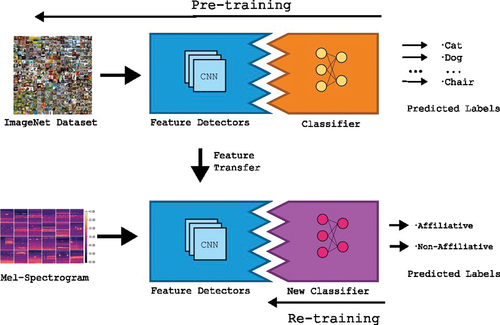
One advantage of using these networks is that pre-trained versions, obtained from training them on large datasets, are available. This enables the use of Transfer Learning (TL) approaches. (see Figure 1 in Box 1). With TL, feature detectors that are already learned by the network can be used in the new task, simplifying training. Here, the three networks were initialised with pre-trained weights. Particularly, VGG16 and ResNet were pre-trained with an image dataset (ImageNet), while VGGish was pre-trained using Google’s Audioset, which takes audio from YouTube videos. Although intuitively it would make sense to transfer from a related task, that is, from an audio classification task instead of natural images, it is known that transferring from an image task to an audio task is feasible (Lasseck 2018). Here, we froze all convolutional layers for all networks, and replace the classifier layers of each network with two layers of densely connected neurons (N = 1024 per layer, reLU activation), connected to a final layer composed of two neurons (one per category, softmax activation).

Box 1. Transfer learning applied to acoustic classification tasks.

Transfer learning (TL) is a technique applied in machine learning and especially easy to apply in deep learning DL, in which a model trained on a task is reused to increase performance in another related task. In a DL system, knowledge transfer happens through using segments of a pretrained network in another network. The new network is trained for the new task, and benefits in the retraining process by not needing as much data as when it would be trained from scratch.

A typical TL approach is performed in two steps. First, the network is pre-trained for a task using a large dataset. Networks for this type usually consist of two segments, namely a feature detector (convolutional layers for the case of a CNN) and a classifier (in most cases, densely connected layers). After the network is fully trained, a feature transfer step occurs, in which the classifier at the end of the network (dense layers) is removed and replaced with a new untrained classifier (densely connected layers initialised with random parameters). Then, the layers in the feature detector are frozen and the new classifier is trained with the data for the new task. This is called retraining. Another approach is fine-tuning, in which some (or all) layers in the feature detector are retrained, but at a much slower rate with much smaller changes. However, fine-tuning requires larger amounts of data. To benefit from a TL approach, both tasks should be related, so that during retraining, the network will take advantage of already learned features from the original task.

Figure 1. Proposed transfer learning scheme. Pre-trained feature detectors (Convolutional segments of a pre-trained network) are transferred to the new application, replacing the classifier segments with untrained densely connected layers. The new classifier is trained to identify the new labels, using learned features from the previous task.

2.3. Data processing

In the current study, each playback clip was converted into a time-frequency representation before being used as input. Mel-spectrograms were computed, using standard settings (NFFT = 4048, Hop length = 256, ~32 ms). Intensities in the spectrogram were represented in decibels, and the number of mel-bins were adjusted to the height that the networks require (224). Finally, the width of the spectrogram (time dimension) was set to 224 by padding with low values (i.e. ~-60 dB, background silence) until all inputs had the same size (i.e. 224 × 224).

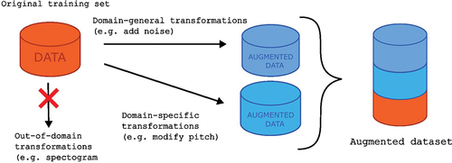
A data augmentation approach was used to increase the amount of training data (see Figure 2 in Box 2). Each audio segment was manipulated using the Parselmouth library (Jadoul et al. 2018) to use pitch manipulation algorithms that are provided by PRAAT (Boersma and Weenink 2007). Parselmouth is a powerful tool for computational acoustics, including bioacoustic feature extraction and data pre-processing (Jadoul et al. 2023) as it integrates seamlessly with other computational frameworks available in Python, such as the deep learning libraries used here. Two types of transformations were applied to training sets. First, sound segments were manipulated to increase or decrease the pitch by half an octave. The PRAAT algorithm could extract and modify pitch even in unvoiced segments, providing a transformed version of vocalisations even in absence of an actual clear sound. Second, noise was added to create a noisy version of the original signal, with approximately 5%,10%, or 15% of the sound’s total energy. Adding noise is a useful way to prevent generalisation and has improved performance in speech recognition applications (Ko et al. 2015). It is generally suggested for audio classification tasks (Abayomi-Alli et al. 2022).

Figure 2. Proposed data augmentation scheme. Original training data are subjected to domain-general (addition of noise) and domain-specific (pitch shift) transformations. Modifications in the time-frequency realm (like spectrogram rotations or stretching) are neglected for this particular study.

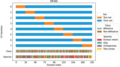
Another problem with small datasets is that a normal train/test split (e.g. 80/20) would yield a too small set (20% of the dataset, that is ~38 samples) to allow an accurate assessment of the model’s performance. A solution in this case is to use a resampling method that uses different subsets of the data to train and test the model on different iterations. Here, we performed a K-fold cross validation (See Box 3), dividing the data into eight subsets (i.e. folds) containing 24 samples, 12 per category (See Figure 3 for visual explanation). This way, we guaranteed a low dispersion between results and that each sample was evaluated at least once. In each iteration, 1-fold (24 samples) was used for testing, while the remaining 7 were used for retraining. For each retraining process, 20 epochs were considered, with a learning rate of 0.05, using Tensorflow’s Adam optimiser. Accuracy measures were obtained for each iteration, and in some cases, accuracy for specific species is also reported.

Figure 3. K-fold cross validation split. Every vocalisation (index in x axis) appears at least in the testing set (orange) and the remaining for training (blue). Class (affective condition) and Species was expressed in the last two lines. All 192 samples were separated in 8 subsets (folds), containing 24 vocalisations. Each fold was balanced in terms of class (12 vocalisations for each emotional valence) but not in terms of groups (random amount of vocalisation per species).

2.4. Implementations

First, the effect of Transfer Learning was evaluated by training the three networks with randomly initialised weights and comparing these to the pre-trained ones (no-TL vs. TL implementation). In this implementation, DA was always used, adding noise (10%), and adding samples with increased and decreased pitch. This should effectively triplicate the number of data samples in each training set, composed of 7 folds (a total of 672 data samples in the augmented dataset).

Second, to evaluate the impact of adding augmented samples in the training process, we tested the model with a progressively higher number of samples (progressive data size augmentation implementation). We wanted to test how many times data needed to be augmented to obtain sufficient performance. Two sub-implementations were evaluated, first with progressively adding more samples of the same type (5% of noise) for all three networks, ranging from no DA to four times the amount of data (x4). Note that since instances of added noise were random, two signals with the same base vocalisation and same noise added were considered different. In the second sub-implementation, different levels of noise were added (5%, 10%, 15%), with progressively more samples (no DA, x2, x3, x4). This approach was only tested in the ResNet network as we hypothesised that conclusions would be equivalent for the other two networks. All these experiments used TL procedures, and the three networks were evaluated independently.

Third, to evaluate which DA transformation best improved accuracy, several combinations of DA sets were considered (DA transformations implementation). We first tested the network augmenting only with noise (10%), for a domain general data transformation against increasing (f0↑) and decreasing (f0↓) pitch separately for a domain specific transformation. This duplicated the training set – for every case the amount of samples was the same. Second, we tested combinations of these approaches (effectively triplicating the amount of samples). A domain general transformation (adding noise, 5% and 10%) was compared against combinations of increase/decrease of pitch together with noise (10%). Finally, we evaluated the network with all three transformations: Noise (10%), pitch increase, and pitch decrease.

To explore how acoustic features from different species vocalisations could generalise across taxa in the two conditions, we chose a complementary approach. We performed a leave-one-out (LOO) cross-validation approach, where the network was trained with 3 of the species, using the data of the left-out species as a test set. The idea was to test the network with data from a species not being trained with, but of the same affective quality. This could provide an idea of how well CNN can generalise affiliative and agonistic vocalisations independent of the species emitting them.

Box 2. Data Augmentation in an acoustic classification task.

A well-described problem in DL is that efficient audio classification systems depend on large datasets for training (Tsalera et al. 2021). High-accuracy sound recognition systems face a big challenge regarding robustness and generalisation as factors such as noisy environments, reverberation, and other types of perturbations can affect performance negatively (Wang et al. 2015). When dealing with small acoustic datasets, a data augmentation procedure can help to increase performance of an otherwise poorly performing system (Zhao et al. 2022).

A data augmentation approach consists of applying transformations to available data to increase the number of items in the training set. The type of transformations applied depends on the task. In a classic image classification task, for example, possible transformations include modifying contrast or rotation of the image. It is important that transformations are applied in a way that important features are preserved after the transformation (e.g, in a face classification task, an eye needs to still be an eye after the transformation). In the case of acoustic classification using CNN, sounds are converted into a time-frequency representation to apply transformations before or after the conversion to spectrograms.

Regarding transformations in the time domain, there is general consensus that applying noise to the signal increases the overall performance independent of the application (Abayomi-Alli et al. 2022). This is considered a ‘domain general’ transformation. If a particular classification task includes vocalisations (animal or human), another suggestion includes a pitch shift, and this is considered a ‘domain specific’ transformation. In both cases, there are parameters that need to be tuned (e.g. the amount of noise, range of frequency shift for the pitch, etc.), and care must be taken to preserve important features. For example, a pitch shift cannot put fundamental frequency in an unnatural range. Other types of transformations include signal scaling or volume increase/decrease. For transformations applied directly to the spectrograms, care must be taken with standard image augmentation protocols, as they may result in unusable training items (e.g. a rotation would mix up time and frequency dimensions). In fact, standard image augmentation procedures have shown to be detrimental in bioacoustic classification tasks (Nanni et al. 2020). Successful transformations in time-frequency representation include masking (i.e. removing segments of the image) and mixing signals (Zhang et al. 2019).

Box 3. K-fold Cross-validation approach.

In Machine Learning, cross-validation is a model validation approach in which the data set is divided into a training and test-set repeatedly in different ways. By running multiple iterations, an idea can be formed about how variable the model’s performance is for different test sets, thus allowing statistical analysis of the model’s performance. A cross- validation approach is preferred over a traditional training/testing split when the dataset is too small, as few data samples for evaluation can underestimate or overestimate a model’s ability to predict new data (James et al. 2013).

There are various cross-validation approaches. The main differences revolve around the size of the splits, the amount of iterations and the type of data. A good criterion is to evaluate how many samples are available and how much computational power the training procedure will take. Usually, more exhaustive approaches tend to take more computational resources, and are preferred for very small datasets. An example is the leave-p-out cross validation, in which p items are taken for testing, and the remaining for training, using all possible combinations p items. A particular case is when p = 1, typically referred to as leave-one-out cross validation. For less exhaustive approaches, a common method is the K-fold cross-validation, in which data is separated into K subsamples, and each subsample is used once for testing across K iterations.

3. Results

First, we trained the VGG16 network with randomly initialised weights, i.e. without any TL approach, but with the previously described DA approach (no-TL condition). Results are reported in Table 3. Without transfer learning, accuracy was around 50% (i.e. no better than chance) on the test set for all three networks. It was clear that the amount of training data was insufficient. With the TL approach (Table 2) average accuracy was around 80% for the VGG16 and ResNet networks and 59% for the VGGish. However, accuracy results on individual species varied significantly. In Table 3, results for individual species showed that all three networks performed better for chimpanzees and tree shrews. Particularly, accuracy of chimpanzees and tree shrews was above 90% for the VGG16, while the ResNet could perfectly classify vocalisations across these species. The VGGish performed, with a 71% accuracy for these two species. On the other hand, accuracy decreased noticeably for human infants and dogs, with 68% and 57% respectively for the VGG16 and 58% and 66% respectively for the ResNet. Finally the VGGish obtained an accuracy of 61% for human infants but could not correctly classify vocalisations of dogs (accuracy below 50%). Note also that for human infants and dogs, variability in accuracy classifications also increased noticeably compared to the other two species.

Table 3. Average accuracy (mean ± standard deviation, in %), for the three tested networks with and without Transfer Learning (TL). Accuracy for individual species for the case with TL is also presented (rows in cursive).

Accuracy (%)	No TL+DA	TL+DA	Human Infants	Dog	Chimpanzee	Tree Shrew
VGG16	0.49±0.03	0.79±0.09	0.68±0.23	0.57±0.24	0.91±0.15	0.98±0.06
Resnet	0.51±0.04	0.81±0.07	0.58±0.17	0.66±0.26	1.0±0.0	1.0±0.0
VGGish	0.49±0.05	0.59±0.10	0.61±0.33	0.43±0.14	0.71±0.18	0.71±0.19

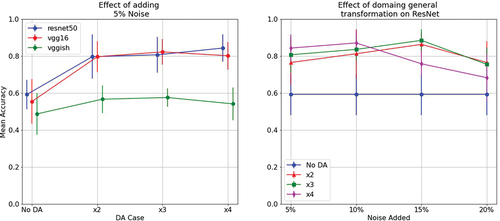
In a second iteration, we evaluated the impact on accuracy based on the number of samples in a training set. For this, we progressively increased the numbers of samples in the training set in two ways. Here we used transfer learning, as the first iteration had shown that no useful learning takes place without it. Results are presented in Figure 4. As shown in Figure 4 (left), using only the original data yielded poor results, although it is worth noting that accuracy was still above chance for the VGG16 and ResNet networks. Augmenting the data increased accuracy as expected, but adding more noisy samples in the x3 and x4 conditions did not noticeably improve accuracy. Overall, ResNet and VGG16 performed better than VGGish. Figure 4 (right) shows that noise at different levels boosted overall performance independent of condition for the ResNet network. In particular, adding 15% of noise yielded the best results, when duplicating or triplicating the training sample. However, increasing the amount of training data using higher levels of noise yielded lower performance compared to other methods.

Figure 4. Effect of adding progressively more samples into a training set, using the same type of augmentation (left). Effect of considering noise at different energy levels for the ResNet network (right).

In the third iteration we explored different combinations of data augmentation techniques, and results are summarised in Table 4. In this case, adding only noise (random transformation) was compared against domain specific transformations, i.e. pitch shift up (f0↑), or down (f0↓), for half an octave. Results revealed that including only domain-specific transformations (both pitch-shift up and down) yielded better results than adding only noise, although this difference seemed not to be statistically significant. In particular, including pitch-down transformations seemed to boost accuracy in all networks. More importantly, using a combination of domain general and domain-specific transformations seemed to yield the best results.

Table 4. Average accuracy (mean ± standard deviation, in %), for the different DA cases, for all three networks. Best results were observed when including a pitch-shift down transformation (f0↓).

	DA x2			DA x3				DA x4
Accuracy (%)	Noise (10%)	f0↓	f0↑	Noise (5%+10%)	f0↓ + Noise (10%)	f0↑ + Noise (10%)	f0↑ + f0↓	Noise (10%)+ f0↑+f0↓
VGG16	0.77±0.09	0.80±0.10	0.71±0.10	0.76±0.06	0.81±0.09	0.77±0.09	0.84±0.08	0.85±0.07
Resnet	0.79±0.11	0.83±0.07	0.81±0.9	0.82±0.07	0.84±0.06	0.79±0.10	0.88±0.08	0.89±0.04
VGGish	0.58±0.08	0.55±0.09	0.49±0.10	0.57±0.09	0.52±0.11	0.52±0.11	0.64±0.12	0.69±0.12

Finally, to evaluate the capacity of the three networks to generalise affective vocalisation qualities across species, the leave-one-out (LOO) cross validation approach was evaluated, using previously described TL and DA approaches. Results are presented in Table 5. It can be seen that the VGG16 network experienced an increase in accuracy when testing on human infants and chimpanzees. The same was observed, but with a higher accuracy, when testing the ResNet network with chimpanzees, but not for human infants. A similar situation occurred with the VGGish, showing an increase in accuracy for chimpanzees and tree shrews, but not for human infants nor dogs. Finally, some accuracies were noticeably low, particularly the ResNet classification of dog and tree shrews, which were below 40%, and the VGGish for dogs at 40%. This suggests that in these cases networks are inverting the affective quality of the recognised class (i.e. recognise an affiliative vocalisation as a non-affiliative, and vice versa).

Table 5. Average accuracy (mean ± standard deviation, in %) for the leave-one-out cross validation approach. Networks were trained with vocalisations from three of the species, while the testing was conducted on the remaining species. An increase in accuracy in chimpanzee vocalisation classification was observed when training with human infants vocalisations using any network. The opposite was observed only for VGG16. An accuracy increase was also observed with the Tree Shrew trained using the VGGish network.

	Test Set
Approach	Human Infants	Dog	Chimpanzee	Tree Shrew
LOO – VGG16	0.59±0.04	0.49±0.02	0.63±0.06	0.47±0.02
LOO – ResNet	0.42±0.03	0.26±0.03	0.79±0.03	0.39±0.04
LOO – VGGish	0.53±0.04	0.40±0.04	0.58±0.05	0.60±0.07

4. Discussion

In this study, we explored different classification approaches in a small set of mammalian vocalisations, using off-the-shelf convolutional neural networks. We highlight the importance of two particular techniques: Transfer Learning and Data Augmentation. Both techniques increased classification accuracy in a dataset of affective vocalisations in mammals. On the one hand, using pretrained networks has been the standard in bioacoustics for some time (Lasseck 2018; Guyot et al. 2021), demonstrating the usefulness in these classification and detection tasks. On the other hand, we also showed that incrementing the amount of data via DA techniques is also beneficial for small datasets, in accord with previous findings in acoustic data (Vecchiotti et al. 2019). DA techniques clearly boost accuracy classification in bioacoustic datasets (Nanni et al. 2020). These prior studies included more than a hundred samples per species and per class. The current results show that a DA approach can improve performance even in small data sets. However, while there is a wide range of transformations that can be applied to acoustic data (Abayomi-Alli et al. 2022), there is little understanding of the effectiveness of some of these transformations in bioacoustic datasets. Previous studies suggested that pitch shifts – among other transformations – are effective in bioacoustic classification of cats and birds (Nanni et al. 2020), being analogous to data in human voice speaker recognition (Nugroho et al. 2022). However, an exploration of parameter settings for these types of transformations (e.g. how much noise should be added or how much pitch should be increased or decreased) is yet to be studied. The current results suggest that noise around 10% or 15% of the total energy of a vocalisation should be added for data augmentation, but this may vary depending on the setting, that is, if there was already background noise or not. A limitation of the current study is that we did not explore if different increases or decreases in pitch improved accuracy, as this is likely to vary depending on the species and a more diverse range of species would be needed for this purpose. To illustrate this point, the vocal range of primates differs from that of birds, so applying the same pitch modification would not necessarily help models to achieve generalisation.

In the present study, ResNet seemed to achieve the best overall performance, closely followed by the VGG16. This might seem counterintuitive, as one would expect feature transfer from a similar task to yield better results. In fact, most recent studies followed the trend of pretraining on acoustic datasets (Kahl et al. 2021). However, evidence showed that transferring from a large image dataset (particularly, the ImageNet dataset used in this study), offers as good results as transferring from an audio dataset for a standard audio classification task (Palanisamy et al. 2020; Fonseca et al. 2021). The reason for this is still unclear (Neyshabur et al. 2021) because there is still no real understanding of what features are transferred in a TL approach. However, one study (Palanisamy et al. 2020) suggested that in initial layers, spectrograms are treated similarly by the network as images. A visualisation of this phenomena shows that the network pays attention to regions with high energy distribution in spectrograms by learning the boundaries of these regions. This is an analogue of how image detection algorithms learn edges around objects. By having unique shapes for each sound, the network can classify them well. Therefore, a network pre-trained on ImageNate that excels as an edge detector, will also be able to derive good classification accuracy with sufficient fine-tuning. Despite this, it remains unknown which pre-trained CNN would perform best in a given task, and recent studies that compare performance of different pre-trained networks are inconclusive (Tsalera et al. 2021). Following the current results, we suggest that both types of approaches (pretraining on image and audio datasets) should be tested in any particular classification task.

The current study also addressed the capacity of these networks to generalise affective call qualities across different species. Although it might seem that on average all three networks could generalise to some degree, looking into individual species we can see that the networks are able to only meaningfully generalise for chimpanzees and tree shrews, with a noticeable decrease in performance for the other two species. Looking into the acoustic characteristics of the calls (see Table A in Appendix), we noted that for chimpanzees and tree shrews, the distinction between agonistic and affiliative vocalisations was similar to the distinction between voiced and unvoiced vocalisations, respectively. On a similar note the Peak frequency is higher for agonistic calls in the same species. We also noticed that there were no major differences in acoustic features of human infants and dogs between the two agonistic conditions. The only exception might have been the peak fundamental frequency, which was slightly higher in the agonistic condition. This was supported by results of the GLM analysis (Table B in Appendix), in which only peak frequency showed a statistical difference between conditions. Interestingly, the distinction between voiced and unvoiced vocalisations was not significant, when considering all species. Despite this, and observing results in Table 4, we suggest that networks might be learning how to differentiate between voiced and unvoiced vocalisations. This is supported by the Leave-one-out cross-validation experiment, in which the VGGish network could slightly improve accuracy when tested in either of the species, whilst being trained on the other three. A possible reason why the VGGish network could make this distinction might be the pretraining of acoustic data (instead of an image dataset), as there might be a better feature transfer for the voiced/unvoiced differentiation. One potential reason why the GLM analysis might not sufficiently differentiate between conditions is that the selected acoustic parameters may not be informative for this analysis. While additional parameters like MFCC and kurtosis could be incorporated, the choice of acoustic parameters is often specific to each case and species, with no universal set of parameters or rules ensuring consistent results. Additionally, the assumption of linearity required for a GLM analysis may oversimplify this particular case. Introducing alternative nonlinear assumptions is challenging as this would necessitate a thorough examination of the vocalisations. One advantage of using DL is it can identify nonlinear relationships within the data without further input. Another advantage of using raw acoustical inputs is that neural networks can learn differences autonomously, eliminating the need for manual feature selection and evaluation, as in traditional machine learning approaches.

Bioacoustic research has suggested that agonistic calls are more relevant in cross-taxa communication (Scheumann et al. 2014) as they usually convey information about danger or threat to other species. In this regard non-linear vocal phenomena are usually present in these vocalisations (Anikin et al. 2020). One could argue that harshness and chaotic sounds derived from non-linear phenomena could be an acoustic feature that can therefore be generalised across taxa. However, as affiliative vocalisations are more commonly used in interspecies communication, it could also be said that these types of vocalisations cannot be generalised. From an evolutionary perspective, it is more likely that phylogenetically related species share similarities in vocalisations. This is something we observed (see Table 4), particularly in the VGG16 network, where accuracy was slightly higher when human infant vocalisations were present in the training set for classifying chimpanzee vocalisations and vice versa. However, we note that with such a limited number of calls and species these interpretations are necessarily preliminary, and given the nature of the tested networks, it remains to be seen which acoustic features ultimately lead to best performance in call classification. On a similar note, a separate study performed on bird vocalisations also suggested a relationship between accuracy in classification and phylogenetic distance (Provost et al. 2022). Consequently, we provided a first step in the use of DL approaches that can ultimately lead to explorations of broader spectra of species and vocalisations.

5. Conclusions

This research investigated the classification of mammalian vocalisations using convolutional neural networks, with a particular focus on techniques like Transfer Learning (TL) and Data Augmentation (DA). Both techniques enhanced the accuracy of classifying the affective quality of vocalisations for this particular dataset. The results showcase the efficacy of pre-training from image datasets, compared to TL from acoustic datasets. Among the models tested, ResNet exhibited the best performance, closely followed by VGG16. The study also explored whether these networks generalise across species, revealing effective discrimination in chimpanzees and tree shrew vocalisations, with less satisfactory results for human infants and dogs. We suggest a potential connection between accuracy and phylogenetic distance, but more studies are required, potentially with a more diverse range of species and types of vocalisations. Overall, we could provide preliminary insight into vocalisation features and their transferability across taxa using deep learning approaches, demonstrating the feasibility of these techniques in future research.

Future research should consider a more extensive range of species vocalisations to achieve more meaningful and robust results in terms of understanding different DA approaches and its limitations, but also for better comprehension of how these models can generalise affective quality across taxa and the feasibility of transferability to more niche applications and/or species. Simultaneously, we hope that this work motivates the use of DL techniques in applications where animal vocalisations are scarce, such as passive acoustic monitoring, which has become an efficient tool to track endangered species (Teixeira et al. 2019). Sound detection and classification for endangered species usually relies on techniques other than DL, like spectral cross-correlation (Arvind et al. 2023) or template matching (De Araújo et al. 2023). In that sense, we hope to encourage the use of DL techniques for acoustic monitoring of endangered species.

Disclosure statement

No potential conflict of interest was reported by the author(s).

Additional information

Funding

The work was supported by the Fonds Wetenschappelijk Onderzoek [G034720N]. The Center for Music in the Brain is funded by the Danish National Research Foundation [DNRF117].

Appendix

Table A. Acoustical characterisation of vocalisations. Mean ± standard deviation of following parameters: Vocalisation duration, mean fundamental frequency (f0), standard deviation of f0, peak frequency, harmonic-to-noise ratio (HNR), percentage of voiced frames, and spectral centre of gravity. Results are presented per species and per category.

	Human Infant	Dog	Chimpanzee	Tree Shrew
Agonistic context – negative emotional valence
Vocalisation duration	0.72 ± 0.18	0.85 ± 0.15	0.75 ± 0.18	0.77 ± 0.13
Mean f0	604.74 ± 492.93	705.61 ± 352.91	1217.7 ± 161.08	2812.97 ± 909.27
Standard Deviation f0	215.59 ± 549.86	302.79 ± 299.74	103.65 ± 102.98	605.09 ± 575.51
Peak frequency	1157.89 ± 669.3	686.96 ± 269.91	1803.18 ± 447.83	4874.27 ± 921.21
HNR	−37.12 ± 47.22	−100.09 ± 36.37	−25.3 ± 26.8	−106.24 ± 18.54
Percentage of Voiced Frames (%)	0.73 ± 0.27	0.48 ± 0.23	0.94 ± 0.1	0.48 ± 0.1
Spectral Centre of Gravity	1548.16 ± 795.25	938.93 ± 261.92	2004.96 ± 282.15	5470.93 ± 662.22
Affiliative context – positive emotional valence
Vocalisation duration	0.76 ± 0.13	0.72 ± 0.16	0.82 ± 0.14	0.69 ± 0.16
Mean f0	576.53 ± 380.01	686.79 ± 209.68	3026.45 ± 1087.77	4376.25 ± 827.05
Standard Deviation f0	358.12 ± 579.81	273.5 ± 341.4	1221.86 ± 833.55	1448.58 ± 465.97
Peak frequency	877.51 ± 674.82	763.95 ± 304.89	430.89 ± 666.13	371.53 ± 1213.94
HNR	−29.11 ± 38.21	−112.15 ± 12.89	−88.02 ± 47.31	−78.86 ± 52.29
Percentage of Voiced Frames (%)	0.86 ± 0.17	0.5 ± 0.17	0.48 ± 0.3	0.65 ± 0.2
Spectral Centre of Gravity	1122.37 ± 673.81	1106.08 ± 272.81	2151.56 ± 1407.34	3492.44 ± 1621.38

Table B. Statistical analysis of acoustical parameters. A generalised linear regression model was considered, with all acoustic parameters used to predict context category (affiliative, agonistic), independent of the species.

	Estimate	Standard Error	t-Value	p-Value
Vocalisation duration	0.51614	0.21765	2.3714	0.018751
Mean f0	−0.18394	0.18295	−1.0054	0.31601
Standard Deviation f0	6.52 × 10^−5	3.77 × 10^−5	1.7316	0.085015
Peak frequency	0.00010731	5.95 × 10^−5	1.8044	0.072807
HNR	−0.00017356	3.13 × 10^−5	−5.5513	9.79E × 10^−8
Percentage of Voiced Frames (%)	−0.0015772	0.00091746	−1.719	0.087287
Spectral Centre of Gravity	0.076262	0.16711	0.45637	0.64866
Vocalisation duration	1.07 × 10^−5	3.80 × 10^−5	0.28132	0.77878

References

- Abayomi-Alli OO, Damaševičius R, Qazi A, Adedoyin-Olowe M, Misra S. 2022. Data augmentation and deep learning methods in sound classification: a systematic review. Electronics. 11(22):3795. doi: 10.3390/electronics11223795.
- Anikin A, Pisanski K, Reby D. 2020. Do nonlinear vocal phenomena signal negative valence or high emotion intensity? R Soc Open Sci. 7(12):201306. doi: 10.1098/rsos.201306.
- Arnaud V, Pellegrino F, Keenan S, St-Gelais X, Mathevon N, Levréro F, Coupé C. 2023. Improving the workflow to crack Small, Unbalanced, Noisy, but Genuine (SUNG) datasets in bioacoustics: the case of bonobo calls. PLOS Comput Biol. 19(4):e1010325. doi: 10.1371/journal.pcbi.1010325.
- Arvind C, Joshi V, Charif R, Jeganathan P, Robin VV. 2023. Species detection framework using automated recording units: a case study of the critically endangered Jerdon’s Courser. Oryx. 57(1):55–62. doi: 10.1017/S0030605321000995.
- Bergler C, Schmitt M, Cheng RX, Schröter H, Maier A, Barth V, Weber M, Nöth E. 2019. Deep representation learning for orca call type classification. In: Ekštein K, editor. Text, speech, and dialogue. Cham: Springer International Publishing; p. 274–286. Lecture Notes in Computer Science. 10.1007/978-3-030-27947-9_23.
- Boersma P, Weenink D. 2007 Jan 1. PRAAT: doing phonetics by computer (version 5.3.51).
- De Araújo CB, Zurano JP, Torres IMD, Simões CRMA, Rosa GLM, Aguiar AG, Nogueira W, Vilela HALS, Magnago G, Phalan BT, et al. 2023. The sound of hope: searching for critically endangered species using acoustic template matching. Bioacoustics. 32(6):708–723. doi: 10.1080/09524622.2023.2268579.
- Fonseca AH, Santana GM, Bosque Ortiz GM, Bampi S, Dietrich MO. 2021. Analysis of ultrasonic vocalizations from mice using computer vision and machine learning. eLife. 10:e59161. doi: 10.7554/eLife.59161.
- Frazao F, Padovese B, Kirsebom OS. 2020. Workshop report: detection and classification in marine bioacoustics with deep learning. arXiv. 10.48550/arXiv.2002.08249.
- Fukushima K. 1980. Neocognitron: a self-organizing neural network model for a mechanism of pattern recognition unaffected by shift in position. Biol Cybern. 36(4):193–202. doi: 10.1007/BF00344251.
- Goodfellow I, Bengio Y, Courville A. 2016. Deep learning. Cambridge (MA): MIT Press.
- Guyot P, Alix F, Guerin T, Lambeaux E, Rotureau A. 2021. Fish migration monitoring from audio detection with CNNs. Proceedings of the 16th International Audio Mostly Conference; New York, NY, USA: Association for Computing Machinery. p. 244–247. AM ’21. 10.1145/3478384.3478393.
- Hassan N, Ramli DA, Jaafar H. 2017. Deep neural network approach to frog species recognition. 2017 IEEE 13th International Colloquium on Signal Processing & Its Applications (CSPA). p. 173–178. 10.1109/CSPA.2017.8064946.
- Hershey S, Chaudhuri S, Ellis DPW, Gemmeke JF, Jansen A, Moore RC, Plakal M, Platt, D., Saurous, R.A., Seybold, B. and Slaney, M. 2017. CNN Architectures for Large-Scale Audio Classification. 2017 IEEE International Conference on Acoustics, Speech and Signal Processing (ICASSP). p. 131–135. 10.1109/ICASSP.2017.7952132.
- He K, Zhang X, Ren S, Sun J. 2015. Deep residual learning for image recognition. arXiv. 10.48550/arXiv.1512.03385.
- Hubel DH, Wiesel TN. 1968. Receptive fields and functional architecture of monkey striate cortex. J Physiol. 195(1):215–243. doi: 10.1113/jphysiol.1968.sp008455.
- Ivanenko A, Watkins P, van Gerven MAJ, Hammerschmidt K, Englitz B, Theunissen FE. 2020. Classifying sex and strain from mouse ultrasonic vocalizations using deep learning. PLOS Comput Biol. 16(6):e1007918. doi: 10.1371/journal.pcbi.1007918.
- Jadoul Y, de Boer B, Ravignani A. 2023. Parselmouth for bioacoustics: automated acoustic analysis in python. Bioacoustics. 33(1):1–19. doi: 10.1080/09524622.2023.2259327.
- Jadoul Y, Thompson B, de Boer B. 2018. Introducing parselmouth: a python interface to praat. J Phon. 71:1–15. doi: 10.1016/j.wocn.2018.07.001.
- James G, Daniela W, Trevor H, Robert T. 2013. Resampling methods. In: James G, Witten D, Hastie T Tibshirani R, editors. An introduction to statistical learning: with applications in R. New York (NY): Springer; p. 175–201. Springer Texts in Statistics. 10.1007/978-1-4614-7138-7_5.
- Joly A, Goëau H, Kahl S, Picek L, Lorieul T, Cole E, Deneu B, Servajean M, Durso A, Bolon I, et al. 2021. Overview of LifeCLEF 2021: an evaluation of machine-learning based species identification and species distribution prediction. 12th International Conference of the Cross-Language Evaluation Forum for European Languages; Sep 2021; Virtual Event (France). p. 371–393. doi: 10.1007/978-3-030-85251-1_24.
- Kahl S, Wood CM, Eibl M, Klinck H. 2021. BirdNET: a deep learning solution for avian diversity monitoring. Ecol Inform. 61:101236. doi: 10.1016/j.ecoinf.2021.101236.
- Knight E, Hannah K, Foley G, Scott C, Brigham R, Bayne E. 2017. Recommendations for acoustic recognizer performance assessment with application to five common automated signal recognition programs. Avian Conserv Ecol. 12(2). doi: 10.5751/ACE-01114-120214.
- Ko T, Peddinti V, Povey D, Khudanpur S. 2015. Audio augmentation for speech recognition. In: Interspeech 2015. ISCA; p. 3586–3589. 10.21437/Interspeech.2015-711.
- Lasseck M. 2018. Audio-based bird species identification with deep convolutional neural networks. p. 11.
- LeBien J, Zhong M, Campos-Cerqueira M, Velev JP, Dodhia R, Lavista Ferres J, Mitchell Aide T. 2020. A pipeline for identification of bird and frog species in tropical soundscape recordings using a convolutional neural network. Ecol Inf. 59:101113. doi: 10.1016/j.ecoinf.2020.101113.
- Nanni L, Maguolo G, Paci M. 2020. Data augmentation approaches for improving animal audio classification. Ecol Inf. 57:101084. doi: 10.1016/j.ecoinf.2020.101084.
- Neyshabur B, Sedghi H, Zhang C. 2021. What is being transferred in transfer learning? doi: 10.48550/arXiv.2008.11687.
- Nugroho K, Noersasongko E, Purwanto M, Moses Setiadi DRI, Setiadi DRIM. 2022. Enhanced Indonesian ethnic speaker recognition using data augmentation deep neural network. J King Saud Univ Comput Inf Sci. 34(7):4375–4384. doi: 10.1016/j.jksuci.2021.04.002.
- Palanisamy K, Singhania D, Yao A. 2020. Rethinking CNN models for audio classification. arXiv. 10.48550/arXiv.2007.11154.
- Provost KL, Yang J, Carstens BC, Staples AE. 2022. The impacts of fine-tuning, phylogenetic distance, and sample size on big-data bioacoustics. PLOS ONE. 17(12):e0278522. doi: 10.1371/journal.pone.0278522.
- Russakovsky O, Deng J, Su H, Krause J, Satheesh S, Ma S, Huang Z, Karpathy A, Khosla A, Bernstein M, et al. 2015. ImageNet large scale visual recognition challenge. Int J Comput Vis. 115(3):211–252. doi: 10.48550/arXiv.1409.0575.
- Salamon J, Bello JP, Farnsworth A, Kelling S. 2017. Fusing shallow and deep learning for bioacoustic bird species classification: 2017 IEEE international conference on acoustics, speech, and signal processing, ICASSP 2017. 2017 IEEE International Conference on Acoustics, Speech, and Signal Processing, ICASSP 2017 - Proceedings; Jun 16; ICASSP, IEEE International Conference on Acoustics, Speech and Signal Processing - Proceedings. p. 141–145. 10.1109/ICASSP.2017.7952134.
- Scheumann M, Hasting AS, Kotz SA, Zimmermann E, Bolhuis JJ. 2014. The voice of emotion across species: how do human listeners recognize animals’ affective states? PLOS ONE. 9(3):e91192. doi: 10.1371/journal.pone.0091192.
- Simonyan K, Zisserman A. 2014. Very deep convolutional networks for large-scale image recognition. arXiv preprint arXiv:1409.1556. doi: 10.48550/arXiv.1409.1556.
- Stowell D. 2022. Computational bioacoustics with deep learning: a review and roadmap. PeerJ. 10(13152):e13152. doi: 10.7717/peerj.13152.
- Stowell D, Stylianou Y, Wood M, Pamuła H, Glotin H, Orme D. 2018. Automatic acoustic detection of birds through deep learning: the first bird audio detection challenge. Methods Ecol Evol. 10(3):368–380. doi: 10.48550/arXiv.1807.05812.
- Sun Y, Wong AKC, Kamel MS. 2009. Classification of imbalanced data: a review. Intern J Pattern Recognit Artif Intell. 23(4):687–719. doi: 10.1142/S0218001409007326.
- Teixeira D, Maron M, van Rensburg BJ. 2019. Bioacoustic monitoring of animal vocal behavior for conservation. Conserv Sci Pract. 1(8):e72. doi: 10.1111/csp2.72.
- Tsalera E, Papadakis A, Samarakou M. 2021. Comparison of pre-trained CNNs for audio classification using transfer learning. J Sens Actuator Netw. 10(4):72. doi: 10.3390/jsan10040072.
- Vecchiotti P, Pepe G, Principi E, Squartini S. 2019. Detection of activity and position of speakers by using deep neural networks and acoustic data augmentation. Expert Syst Appl. 134:53–65. doi: 10.1016/j.eswa.2019.05.017.
- Wang J-C, Lee Y-S, Lin C-H, Siahaan E, Yang C-H. 2015. Robust environmental sound recognition with fast noise suppression for home automation. IEEE Trans Autom Sci Eng. 12(4):1235–1242. doi: 10.1109/TASE.2015.2470119.
- Wang K, Wu P, Cui H, Xuan C, Su H. 2021. Identification and classification for sheep foraging behavior based on acoustic signal and deep learning. Comput Electron Agric. 187:106275. doi: 10.1016/j.compag.2021.106275.
- Xie J, Hu K, Zhu M, Yu J, Zhu Q. 2019. Investigation of different CNN-based models for improved bird sound classification. IEEE Access. 7:175353–175361. doi: 10.1109/ACCESS.2019.2957572.
- Zhang Z, Xu S, Zhang S, Qiao T, Cao S. 2019. Learning attentive representations for environmental sound classification. IEEE Access. 7:130327–130339. doi: 10.1109/ACCESS.2019.2939495.
- Zhao YX, Li Y, Wu N. 2022. Data augmentation and its application in distributed acoustic sensing data denoising. Geophys J Int. 228(1):119–133. doi: 10.1093/gji/ggab345.
- Zhong M, Castellote M, Dodhia R, Lavista Ferres J, Keogh M, Brewer A. 2020. Beluga whale acoustic signal classification using deep learning neural network models. J Acoust Soc Am. 147(3):1834. doi: 10.1121/10.0000921.
- Zhong M, LeBien J, Campos-Cerqueira M, Dodhia R, Ferres JL, Velev JP, Mitchell Aide T. 2020. Multispecies bioacoustic classification using transfer learning of deep convolutional neural networks with pseudo-labeling. Applied Acoustics. 166:107375. doi: 10.1016/j.apacoust.2020.107375.