Full article: Escaping the No Free Lunch Theorem: A Priori Advantages of Regret-Based Meta-Induction

Formulae display: $MathJax Logo$ ?Mathematical formulae have been encoded as MathML and are displayed in this HTML version using MathJax in order to improve their display. Uncheck the box to turn MathJax off. This feature requires Javascript. Click on a formula to zoom.

ABSTRACT

A new solution strategy for the problem of induction has been developed based on a priori advantages of regret-weighted meta-induction (RW) in prediction tasks. These a priori advantages seem to contradict the no-free lunch (NFL) theorem. In this paper, the NFL challenge is dissolved by three novel results: (1) RW enjoys free lunches in the long run. (2) Yet, the NFL theorem applies to iterated prediction tasks, because the distribution underlying it assigns a zero probability to all possible worlds in which RW enjoys free lunches. (3) The a priori advantages of RW can even be demonstrated for the short run.

KEYWORDS:

1. Introduction: the NFL theorem and Hume’s problem of induction

How can inductive inferences be rationally justified, in the sense of being reliable or at least preferable to non-inductive inferences? This is the problem of induction. It was raised by the philosopher David Hume almost three centuries ago. Today, its solution is still unsettled. Hume showed that all standard methods of justification fail when applied to the task of justifying induction. Obviously, induction cannot be justified by deductive logic, since it is logically possible that the future (unobserved) is completely different from the past (observed). Most importantly, induction cannot be justified by induction from the observation of its past success in the following way:

(1) Inductive justification of induction: Induction has been successful in the past, thus by induction it will be successful in the future.

Argument (1) is circular and without justificatory value. This has been most clearly demonstrated by Salmon (Citation1957, p. 46) who pointed out that anti-induction may also be pseudo-justified in the same circular manner. Roughly speaking, anti-induction predicts the opposite of what has been regularly observed in the past (cf. sections 5–6). Its circular ‘justification’ runs as follows (where ‘successful/unsuccessful’ means ‘having more/less success than random guessing’):

(2) Anti-inductive justification of anti-induction: Anti-induction was unsuccessful in the past, thus by anti-induction it will be successful in the future.

This shows that with the help of circular reasoning one may justify mutually inconsistent conclusions. This proves that this kind of reasoning is without cognitive value. Considerations of this sort led Hume to the skeptical conclusion that induction cannot be rationally justified at all, but is merely the result of psychological habit.

The no-free lunch theorem (NFL) deepens Hume’s inductive skepticism. NFL theorems have been formulated for different learning tasks and in different versions (cf. Giraud-Carrier & Provost, Citation2006; Rao et al., Citation1994; Schaffer, Citation1994; Wolpert, Citation1992; Wolpert & Macready, Citation1995). In this paper, we investigate the NFL theorem in application to online prediction tasks. The most general formulation is found in Wolpert (Citation1996). Wolpert’s NFL theorem comes in a weak and a strong version. The strong version rests on unrealistic assumptions about the loss function. Therefore, we focus in this paper on the weak NFL theorem. It says that the probabilistically expected success of any (non-clairvoyant) prediction method is equal to the expected success of random guessing or any other prediction method, provided that one assumes (a) a state-uniform prior probability distribution (abbreviated SUPD), ie a distribution that is uniform over all possible world states, and (b) a weakly homogeneous loss function (see below).

Does the NFL theorem undermine the objective of learning theory? A standard defence of learning theorists against the NFL challenge maintains that one should not compute the expected success of learning strategies by means of a state-uniform prior distribution. Rather, one should compute expected success using the (conjectured) actual distribution of the possible states of our environment, and ‘according to our evidence’, the latter distribution is clearly not uniform.Footnote¹ We argue that this line of defence against the NFL challenge does not work, because our beliefs about the actual distribution of possible states of our environment are themselves based on an inductive inference. Thus, this argument commits the fallacy of circularity: inductive reasoning is ‘justified’ because, by means of an inductive inference, we believe that the actual distribution is not state-uniform. However, the only thing we know for sure, by direct experience, are the frequency distributions in samples observed in the past. Whether their inductive generalization to predictions of the future is reliable depends on the unobserved part of this distribution. Here, the NFL theorem comes into play and undermines this line of defence by pointing out that every generalization method (whether inductive, anti-inductive or whatever) is on average equally successful. Thus, we could, with equal right, infer from our past evidence the opposite of what the inductivist infers, namely, that future distributions will be state-uniform. This brings us back to the general argument against circular justifications raised above: that with their help, opposite conclusion can be ‘justified’.

We do not deny that there is achievement in demonstrating that some learning methods are better than others under the supposition that the true probability distribution has already been learned. However, for a robust defence of inductive learning methods against the NFL challenge, a better argument is needed, one that does not presuppose what has to be proved.

Recently, a non-circular solution to the problem of induction has been proposed. It is based on a priori results about the access optimality and access dominance of regret-weighted meta-induction (in short: RW) in online learning.Footnote² In this paper, we explore the relation between meta-induction and the NFL theorem. In sections 2 and 3 the most important results about RW are presented and confronted with the weak NFL theorem in application to iterated binary prediction tasks in online learning. Thereafter, the apparent contradiction is analyzed and dissolved, from both the long-run (sec. 4) and short-run perspectives (sec. 5). We also consider real-valued prediction tasks (sec. 3 and 6). Wolpert’s NFL theorem does not apply to them, but we will prove a restricted version of the NFL theorem that still applies and study its relation to RW. Our investigations continue the work of Schurz and Thorn (Citation2017) and Schurz (Citation2019). Sections 2–4 recapitulate the major findings about meta-induction and the long-run analysis of the NFL theorem, together with new findings.Footnote³ Sections 5 contains a short-run investigation of the performance of meta-inductive strategies in binary prediction games based on computer simulations that, for the first time, analyze the exponential variant of RW and compare it with linear RW; moreover, the results about average regrets, quadratic scoring and scoring with regularity bias, theorem 6 and are new. Section 6 presents computer simulations of real-valued prediction games presenting almost exclusively new results. As an outlook, section 7 exhibits two novel applications of meta-inductive strategies to two real-world problems.

Table 1. Meta-induction and no-free lunch for binary event games. Cells show the percentage of possible binary sequences with 20 rounds, for which the six methods M-I, M-AI, Av, ITB, LRW, and ERW have achieved an absolute success within respective intervals (left margin). The last line shows state-uniform average of absolute success and absolute regret, compared to maximal success.

Download CSV Display Table

Table 2. Meta-induction and no-free lunch for binary event games. Effect of the increase of rounds from 10 to 20 for M-I, M-AI, LRW, and ERW. Cells show the percentages of sequences in which success rates within respective intervals (left margin) have been reached.

Download CSV Display Table

Table 3. Meta-induction and no-free lunch for binary event games with a quadratic scoring. Cells show the percentage of possible binary sequences with 20 rounds, for which the six methods M-I, M-AI, Av, ITB, LRW, and ERW have reached an absolute success within respective intervals (left margin). The last line shows state-uniform average of absolute success and absolute regret, compared to maximal success.

Download CSV Display Table

Table 4. Meta-induction for binary events from the perspective of a frequency-uniform distribution. Cells show (average) absolute successes of the six methods M-I, M-AI, Av, ITB, LRW, and ERW, for binary sequences with 20 rounds, depending on their event frequencies (left margin).

Download CSV Display Table

Table 5. Meta-induction for binary events from the perspective of frequency-uniform distributions, with quadratic scoring. Cells show (average) absolute successes of the six methods M-I, M-AI, Av, ITB, LRW, and ERW, for binary sequences with 20 rounds, depending on their event frequencies (left margin). The last line shows the average success for a distribution with a weak regularity bias.

Download CSV Display Table

Based on our investigations, a defence against the NFL challenge is developed that is based on five novel results:

– RW enjoys free lunches, ie its predictive long-run success dominates that of other prediction strategies.

– The NFL theorem applies to iterated online prediction tasks, provided that the assumed prior distribution is a SUPD.

– The SUPD is maximally induction-hostile and assigns a probability of zero to all possible worlds in which RW enjoys free lunches. This dissolves the apparent conflict with the NFL theorem.

– The a priori advantages of RW can be demonstrated even under the assumption of a SUPD. For infinite event sequences, these advantages follow from the long-run optimality and dominance properties of RW. For finite event sequences, they are based on RW’s combined ability to avoid large losses in irregular sequences and achieve near optimal successes in regular sequences.

– Further advantages of RW become apparent when frequency- or entropy-uniform distributions are considered.

2. Regret-weighted meta-induction

In the area of regret-based learning, theoretical results about vanishing long-run regrets of certain meta-strategies of prediction (or decision) have been developed. These results hold universally, for strictly all possible event sequences, independent of any assumed probability distribution (Cesa-Bianchi & Lugosi, Citation2006; Shalev-Shwartz & Ben-David, Citation2014, ch. 21). Although labelled as ‘online learning under expert advice’, these results characterise the performance of strategies of meta-learning (cf. Lemke et al., Citation2015), inasmuch as a forecaster which we call the ‘meta-inductivist’ tracks the past success rates of accessible prediction methods (‘experts’) and utilises this information in constructing an improved prediction strategy. Since the meta-inductivist predicts future events based on past success rates, short-run regrets (compared to the best method) are unavoidable. What can be achieved in the short run is proving worst-case bounds of these regrets that are as tight as possible and converge to zero as fast as possible. In the long run, the regret-weighted meta-inductivist, RW, is guaranteed to predict at least as accurately as the best accessible prediction method, even in circumstances of non-convergent success rates of the independent methods. A frequent label for this property is ‘Hannan-consistency’ (Cesa-Bianchi & Lugosi, Citation2006, p. 70). Schurz and Thorn (Citation2016) propose to call this property access optimality, because

– it expresses a long-run optimality result restricted to accessible methods, and

– this label is in line with standard game theoretical terminology of ‘optimality’ and ‘dominance’.

Based on these facts, a solution to Hume’s problem of induction is proposed (Schurz, Citation2008, Citation2019) that proceeds as a two-step argument as follows: (i) The meta-strategy RW has an ‘a priori’ justification, because for any given cognitive agent and in every possible world, it is recommendable to apply this meta-strategy on top of all prediction methods accessible to the agent. (ii) Per se, this a priori justification of RW does neither entail that object induction (induction applied at the level of events) is more successful than random guessing nor that there cannot exist a more successful clairvoyant method. However, the a priori justification of meta-induction bestows us a non-circular a posteriori justification of object induction in our world as follows: Until now, non-inductive prediction strategies have been observed to be significantly less successful than the inductive ones, and hence, it is meta-inductively justified to favor object-inductive strategies in the future. This argument is no longer circular, because it is backed up by a non-circular justification of meta-induction.

What stands in apparent conflict with the NFL theorem is not the access optimality of RW, but rather its access dominance, that is, the fact that RW performs at least as well and sometimes better than other accessible methods. At the end of this section, we prove that RW is access-dominant in comparison to many other prediction methods. This means that there are ‘free lunches’ for RW, ie, advantages in some possible world states that are not compensated by disadvantages in other possible world states.

We now turn to the formal definitions and results. Following Schurz (Citation2008), meta-induction is explicated in the framework of prediction games.

Definition 1 (Prediction game): A prediction game is a pair $((e), P)$ consisting of

(1.1) An infinite sequence $(e) := (e_{1}, e_{2}, \dots)$ of events $e_{n}$ coded by real numbers between 0 and 1, possibly rounded according to a finite accuracy. $V a l \subseteq [0, 1]$ denotes the value space of possible events $e_{n} \in V a l$ . Each time n corresponds to one round of the game.

(1.2) A finite set of prediction methods or ‘players’ $P = A \cup M$ , whose task, in each round n, is to predict the next event $e_{n + 1}$ of the event sequence. Methods are of two sorts: $A = {A_{1}, \dots, A_{m}}$ is the set of accessible base methods (eg, object-inductive algorithms or experts), and $M = {M_{1}, \dots, M_{k}}$ the set of meta-methods that base their predictions on those of the base methods. The predictions of all methods are assumed to be elements of a value space $V a l_{p r e d} \subseteq [0, 1]$ that may extend $V a l$ ( $V a l \subseteq V a l_{p r e d}$ ).

We say that (i) a method A is accessible to a meta-method M iff (if and only if), at any time of the given prediction game, M can either (a) observe A’s present predictions (external access) or (b) simulate A’s present predictions (internal access). Moreover, (ii), a class $A$ of methods is accessible to a meta-method M iff (a) all methods in $A$ are accessible to M in the sense of (i) and (b) M can simultaneously keep a record of their present predictions and past success rates and apply its evaluation algorithm to these data.

Prediction games (as defined above) may be applied in different ways. In the context of epistemology, it is assumed that $A$ contains all methods that are accessible to the given epistemic agent, while $M$ contains only one method, the agent’s meta-method that is a priori justified by its access optimality. Typically, the base methods are independent methods (‘individual learners’) that compute their predictions solely from observations of events. However, for several purposes, it is important that $A$ may also contain dependent methods (‘social learners’), provided that the access relations are not circular; in particular, methods in $A$ must not attempt to base their predictions on the meta-methods in M (Schurz, Citation2019, p. 91 f.). Another kind of application that will also be employed in this paper is the comparative evaluation of meta-methods in the form of prediction tournaments. Here, $M$ contains several meta-methods that have access to the same set $A$ of base methods, but are inaccessible to each other (cf. Schurz & Thorn, Citation2017; Thorn & Schurz, Citation2019).

The evaluation of a method’s success is achieved by the following notions:

– $p r e d_{n} (P)$ is the prediction of player $P$ for time $n$ delivered at time $n - 1$ .

– The distance of the prediction $p r e d_{n}$ from the event $e_{n}$ is measured by a normalised loss function, $l o s s (p r e d_{n}, e_{n}) \in [0, 1]$ .

– The natural loss function is defined as the absolute distance between prediction and event, $| p r e d_{n} - e_{n} |$ . It is a special case of linear loss functions ( $c_{0} + c_{1} \cdot | p r e d_{n} - e_{n} |$ ). However, the results about universal access optimality below apply to much larger classes of loss functions: (i) The results about actual losses of real-valued predictions apply to all loss functions that are convex in the argument $p r e d$ , which means that the loss of a weighted average of two predictions is not greater than the weighted average of the losses of two predictions (eg, linear, polynomial and exponential functions of the natural loss function are convex). (ii) The results about expected or average losses with discrete predictions hold for arbitrary loss functions.

– $s c o r e (p r e d_{n}, e_{n}) := 1 - l o s s (p r e d_{n}, e_{n})$ is the normalised score obtained by prediction $p r e d_{n}$ of event $e_{n}$ .

– $a b s_{n} (P) := \sum_{i = 1}^{n} s c o r e (p r e d_{i} (P), e_{i})$ is the absolute success achieved by method $P$ until time $n$ .

– $s u c_{n} (P) := a b s_{n} (P) / n$ is the success rate of method $P$ at time $n$ .

– $M a x s u c_{n} := m a x ({a b s_{n} (P) : P \in A})$ is the maximal absolute success of the accessible base methods at time $n$ and $m a x s u c_{n} := M a x s u c_{n} / n$ is their maximal success rate.

In prediction games as defined by us, it is allowed that probabilistic mixtures (weighted averages) of events may be predicted. Thus, even if the events are binary ( $e_{i} \in {0, 1})$ , predictions may be any real numbers in [0,1]. This is different in discrete prediction games, in which the predictions must coincide with events. In this paper, we focus on games with real-valued predictions and mention discrete prediction games only in the margin.

The simplest kind of meta-induction, in short MI, is the strategy Imitate-the-best, abbreviated ITB. In each round n, ITB imitates the prediction of the method with maximal success at time n; in cases of ties, it choses the first best method in an arbitrary ordering. ITB fails to be universally access-optimal: Its success rate breaks down when it plays against adversarial methods, who return inaccurate predictions as soon as their predictions are imitated by ITB (Schurz, Citation2008, sec. 4). ITB is only access-optimal in prediction games whose set of accessible methods contains a unique best method $A_{k}$ after a winning time w (cf. Schurz, Citation2019, sec. 6.1).

In contrast, regret-weighted meta-induction (RW) predicts a weighted average of the predictions of the accessible methods (see definition 2.1). The weights of RW depend on the so-called regrets, or attractivitiesFootnote⁴ (see definition 2.2). We here consider two kinds of regret-weighted strategies: (i) linear regret-weighted meta-induction, abbreviated as LRW, whose weights are proportional to the positive parts of the regret rates (definition 2.3), and exponential regret-weighted meta-induction, abbreviated as ERW, whose weights are exponential functions of the absolute regrets (definition 2.4). When we assert something about RW, we mean that the assertion holds for both LRW and ERW.

Definition 2 (Regret-weighted meta-induction)

(2.1) For every weighted MI strategy W, its predictions are defined as

p r e d_{n + 1} (W) := \frac{\sum_{i = 1}^{m} w_{n} (A_{i}) \cdot p r e d_{n + 1} (A_{i})}{\sum_{i = 1}^{m} w_{n} (A_{i})},

provided

n > 0

and the denominator is positive; else

p r e d_{n + 1} (W) = 0.5.

(2.2) For every regret-weighted MI strategy RW, the absolute regret of RW with respect to an accessible base method $A_{i}$ at time $n$ is defined as $R e g_{n} (A_{i}) := a b s_{n} (A_{i}) - a b s_{n} (R W)$ and the relative regret as $r e g_{n} (A_{i}) := R e g_{n} (A_{i}) / n$ .

(2.3) The weights of the linear RW strategy, in short LRW, are defined as $w_{n} (A_{i}) := m a x (r e g_{n} (A_{i}), 0)$ .

(2.4) The weights of the exponential RW strategy, in short LRW, are defined as $w_{n} (A_{i}) := e^{\sqrt{(8 \cdot l n (m) / (n + 1))} \cdot R e g_{n} (A_{i})}$ .

The crucial property of RW is that RW forgets prediction methods that have negative regret rates, ie predict worse than RW. While LRW forgets them immediately, ie attaches a weight of zero to every method with negative regret, ERW forgets them gradually, since here negative absolute regrets are set into the exponent, which means that for increasing n, their weight converges rapidly to zero. We will see soon that ERW’s exponential weights lead to an improved worst case bound for EAW’s maximal regret (theorem 1), but lead to a slower rate of forgetting suboptimal methods, which makes a difference for the short-run behaviour of LRW and ERW (sections 5–6).

The notion of access optimality is defined as follows:

Definition 3 (Access optimality)

(3.1) A meta-method method M is access-optimal in a class $G$ of prediction games iff for all $((e), A \cup M) \in G$ ,

$M \in M$ , and $l i m s u p_{n \to \infty} (m a x s u c_{n} - s u c_{n} (M)) \leq 0$ .

(3.2) A (meta-) method M is universally access-optimal iff it is access-optimal in the class of all prediction games whose set of meta-players contains M.

Our notion of access optimality refers to the long run, ie, the limiting performance for $n \to \infty$ . It requires that the limit superior of the success difference between the maximal success of the accessible methods and RW’s success must not be greater than zero; this requirement is well-defined even if neither the success rates nor the success differences converge.

Theorem 1 establishes that both LRW and ERW are universally access-optimal in the long run. In the short run, they may suffer from a possible regret compared to the maximal success of the accessible methods which, however, is bound by tight worst-case bounds that converge to zero when n grows large. The result of theorem 1 holds even in ‘adversarial’ environments with event frequencies and success rates that do not converge but are endlessly oscillating in irregular ways.

Theorem 1 (Universal access optimality of RW)

For every prediction game $((e), A \cup M)$ with $R W \in M$ and a convex loss function, the following holds

(1.1) Short run:

For LRW: ( $\forall n \geq 1$ ) $m a x s u c_{n} - s u c_{n} (L R W) \leq \sqrt{\frac{m}{n}}$ .

For ERW: $(\forall n \geq 1$ ) $m a x s u c_{n} - s u c_{n} (E R W) \leq \sqrt{2 \cdot l n (m) / n} + \sqrt{l n (m) / 8 \cdot n^{2}}$

\leq 1.77 \cdot \sqrt{l n (m) / n} .

(1.2) Long run:

For $R W \in {L R W, E R W}$ : $l i m s u p_{n \to \infty} (m a x s u c_{n} - s u c_{n} (R W)) \leq 0$ .

A generalised proof of theorem 1.1 for all polynomially weighted meta-inductivists is found in Cesa-Bianchi and Lugosi (Citation2006), pp. 9–14 (cf. theorem 2.1, corollary 2.1). LRW is identical to the polynomially weighted ‘forecaster’ (meta-inductivist) with parameter $p$ set to 2. A proof for ERW is given in Cesa-Bianchi and Lugosi (Citation2006), p. 17–20 (cf. theorem 2); for a simpler proof for ERW with a fixed prediction horizon, see Shalev-Shwartz and Ben-David (Citation2014), p. 253 f. ERW’s worst-case bounds are a significant improvement over LRW’s worst-case bounds, as they do not increase with $\sqrt{m}$ but with $\sqrt{l n (m)}$ . However, this result concerning worst-case bounds does not necessarily say much about average performance (see sections 5–6).

As remarked above, theorem 1 does not directly apply to discrete prediction games. These are games with a finite space of event values $V a l = {v_{1}, \dots, v_{r}}$ whose predictions must choose one of these values; predicting mixtures or probabilities of events is not allowed, ie $V a l = V a l_{p r e d}$ . An important subcase is discrete games with binary events coded by their truth values: $V a l = V a l_{p r e d} = {0, 1}$ . Theorem 1 is not directly applicable to discrete games because their loss function (eg the zero-one loss) is usually not convex. Yet there are two ways in which theorem 1 can be indirectly applied to discrete prediction games for RW = LRW as well as for RW = ERW. They are based on the fact that the probabilistic expectation or average value of an arbitrary loss function is always linear and thus convex (cf. Schurz, Citation2019, p. 333):

(1) Randomization, $r R W$ : Here, $r R W$ predicts $e_{n + 1} = v_{i}$ (the next event takes value $v_{i}$ ) with a probability ( $P$ ) that equals the weight sum of all accessible players predicting $v_{i}$ , where the players’ weights are defined in the same way as for RW. It can be proved that the cumulative expected regret of rRW (ie, the sum of RW’s P-expected losses for each round) is smaller than or equal to RW’s worst-case regret: $m a x s u c_{n} - (1 / n) \cdot \sum_{1 \leq t \leq n} E x p_{P} (s c o r e_{t} (r R W)) \leq b_{n}^{R W}$ , where $b_{n}^{R W}$ is the worst-case bound of RW $\in {L R W, E R W}$ and $E x p_{P} (s c o r e_{n} (r R W))$ $:= \sum_{1 \leq i \leq r} P (e_{n + 1} = v_{i}) \cdot (1 - l o s s (v_{i}, e_{i}))$ ; for the proof cf. Cesa-Bianchi and Lugosi (Citation2006), sec. 4.1 +2, and more explicitly in Schurz (Citation2019), appendix 12.25. However, this method is not fully general, because it presupposes that the events are probabilistically independent of $r R W$ ’s choice of prediction. Therefore, this method does not yield access-optimal predictions in adversarial environments.

(2) Collective meta-induction, $c R W$ , introduced in Schurz (Citation2008), sec. 8: Here, a collection of k meta-inductivists $c R W_{1}, \dots, c R W_{k}$ approximates the probabilies of rRW’s predictions of the event values by the frequencies of cRW’s predicting these values. For the average regret of cRW’s predictions, a worst-case regret bound can be proved that equals $b_{n}^{R W}$ plus an additional worst-case regret due to rounding errors of size $\frac{r - 1}{2 \cdot k}$ (r being the number of possible event values). By increasing k, the additional regret can be made arbitrarily small.Footnote⁵ The important property of collective RW meta-induction is that its approximative access optimality holds in full generality and for all loss functions. Moreover, assuming that the $c R W$ s are cooperators and share their success in equal parts, then in addition to achieving a collective average success that is approximately access-optimal, each individual member of the collective is guaranteed to be approximately access-optimal.

A further generalization of theorem 1 is possible by applying meta-induction to sets of accessible methods whose finite size is allowed to grow unboundedly in time. It can be shown that even if confronted with growing sets of accessible methods, ERW is access-optimal, provided that the number of accessible methods grows less than exponentially in time (cf. Mourtada & Maillard, Citation2017; Schurz, Citation2019, sec. 7.3.1). For the purpose of this paper, this extension is not needed.

Universal access optimality is a great a priori advantage of RW. Optimality, however, it is not enough to offer a possible solution to the consequences of the NFL theorem, for the reason that the notion of optimality does not exclude the possibility that there can be many equally optimal methods. A unique preference for one method in a given class of methods requires the stronger notion access dominance defined as follows:

Definition 4 (Access dominance)

A meta-method M is access-dominant with respect to a class $M$ of meta-methods containing M iff M, but no other method in $M$ is access-optimal in the class $G_{M}$ of all prediction games whose set of meta-methods is $M$ .

Note: This is equivalent to the condition that for every meta-method $M^{⋆} \in M ∖ {M}$ , there exist prediction games in $G_{M}$ in which M is superior to M $^{⋆}$ , in the sense that $l i m i n f_{n \to \infty} (s u c_{n} (M) - s u c_{n} (M^{⋆})) \geq 0$ and $l i m s u p_{n \to \infty} (s u c_{n} (M) - s u c_{n} (M^{⋆})) > 0$ (proof in Schurz, Citation2019, p. 96, prop. 5.1).

We do not define the notion of universal dominance; it does not apply because there are different versions of regret-based meta-induction, all of which are optimal in the long run and not uniquely ranked according to their short-run performance (eg ERW and polynomial meta-inductivists mentioned above). So RW cannot be universally access-dominant. What the NFL theorem suggests, however, is a much stronger claim, namely that no method can dominate another method, thus all methods are ‘equally optimal’. In the remainder of this section, we show that this is not true.

Theorem 2 states a variety of restricted dominance results for RW. Concerning theorem (2.2) (a), note that the notions of access optimality and access dominance, although designed for meta-methods, may also be applied to independent methods, which if included in $M$ simply make no use of the information about the behaviour of other methods. Particularly interesting is the failure of access optimality of the meta-inductive method SW that identifies unnormalised weights with success rates. The rule SW has been frequently studied in cognitive psychology, where it has been called ‘Franklin’s rule’ (Gigerenzer et al., Citation1999, p. 83). The reason why SW cannot be access-optimal is the fact that, unlike RW, it does not forget methods that predict worse than itself.

Theorem 2 (access dominance for RW)

(2.1) RW dominates every accessible prediction method $M$ (in the long run) that is not universally access-optimal, ie, for every such method $M$ , there is a prediction game containing RW and $M$ in which RW’s long-run success rate exceeds that of $M$ , $l i m i n f_{n \to \infty} (s u c_{n} (R W) - s u c_{n} (M)) > 0$ .

(2.2) Not universally access-optimal in the long run are (a) all independent (non-clairvoyant) methods and (b) among meta-strategies (b1) all one-favourite methods (which at each time point imitate the prediction of one accessible method), (b2) success-based weighting SW using success rates as weights, and (b3) linear regression for a linear loss function.

Proof. Proof of theorem (2.1): Assume that M is not access-optimal. So there exists a prediction game $((e), A \cup M)$ with $M \in M$ such that M is not access-optimal in $((e), A \cup M)$ . We add RW to $M$ , which does not affect the methods accessible to M. Thus, M is not access-optimal in $((e), A \cup M \cup {R W})$ either, but by theorem 1, RW is access-optimal in this game. Thus (by the note to definition 4), RW dominates M.

Proof of theorem (2.2) (a): Let O be an independent method based on a computable prediction function f, and $(e^{'})$ an O-adversarial event sequence defined as follows: $e_{1}^{'} = 0.5$ , and $e_{n + 1}^{'} = 1$ if $f (e_{1}^{'}, \dots, e_{n}^{'}) < 0.5$ ; else $e_{n + 1}^{'} = 0$ . The predictions of the perfect $(e^{'})$ -forecaster O’ are identified with the so-defined sequence, ie, $p r e d_{n} (O^{'}) = e_{n}^{'}$ . In the prediction game $((e^{'}), {O, O^{'}, R W})$ , the success rate of O can never exceed 1/2, that of $O^{'}$ is always 1 and that of RW converges to 1 (by theorem 1). So O is not universally access-optimal.

Proof of theorem (2.2)(b1): Consider the binary prediction game ((e), {OF, A1, A0}), where OF is a one-favourite meta-strategy, A1 predicts always 1, A0 always 0, and (e) is an ‘OF-adversarial’ event sequence, ie, $e_{n} = | 1 - p r e d_{n} (O F) |$ . Then, OF’s success rate is always zero, while at any time n, at least one of A1 and A0 must have a success rate of $\geq 0.5$ ; thus, OF is not access-optimal.

Proof of theorem (2.2) (b2): Consider a real-valued prediction game ((e), {P, Q, SW}) satisfying $\forall n : 0 <$ pred_n(P) < pred_n(Q) < e_n. This implies (*) $\forall$ n: $s u c_{n} (P) < s u c_{n} (Q)$ . Our assumptions entail that score $_{n + 1} (S W) = 1 - (e_{n + 1} - (w_{n} \cdot p r e d_{n + 1} (P) + (1 - w_{n}) \cdot p r e d_{n + 1} (Q)))$ , where $w_{n} := s u c_{n} (P) / (s u c_{n} (P) + s u c_{n} (Q))$ . This together with (*) implies that score $_{n} (P) <$ score $_{n} (S W) <$ score $_{n} (Q)$ , and hence, $s u c_{n} (P) < s u c_{n} (S W) < s u c_{n} (Q)$ holds for all n; thus, SW is not access-optimal.

Proof of theorem (2.2) (b3): Assume a binary random sequence converging against a limiting 1-frequency of $r > 0.5$ , with two independent predictors A1 and A0 that constantly predict 1 and 0, respectively. Then, linear regression always predicts the so-far event frequency, which minimises the squared loss, but not the linear loss. The linear loss is minimised by the median value, which is 1 in our setting and is predicted by the method A1. Thus, linear regression with a linear loss function is not access-optimal.□

Theorem 2 brings us to the core question of this paper. For the theorem seems to entail that in the long run, there are ‘free lunches’ for regret-based meta-induction, in the sense that there are prediction methods $M$ and event sequences $(e)$ for which RW’s long-run success is strictly greater than that of $M$ without there being any ‘compensating’ event sequences $(e^{'})$ in which RW’s long-run success is smaller than that of $M$ . This is in apparent conflict with the NFL folklore. This conflict is investigated in the next sections.

3. NFL theorems for prediction games

The application of NFL theorems to prediction games is not straightforward. First of all, the prediction game account is more general than the NFL framework since the results of the former account hold even if clairvoyant methods are admitted. Thereby, a prediction method is clairvoyant if its choice of prediction is deterministically or probabilistically dependent on some future events, conditional on all past events. For clairvoyant methods, free lunches are obviously possible, and one philosophically important advantage of the strategy RW is that it is access-optimal even if clairvoyant methods are allowed. However, regret-based meta-induction should not only be attractive for those who consider paranormal worlds as possible. Thus, in what follows, we take the non-clairvoyance assumption of the NFL theorems (Wolpert, Citation1996, p. 1380) as granted and investigate their compatibility with the access dominance of regret-based learning.

There are two further possible hindrances of applying the NFL framework to regret-based online learning. They are treated as follows:

– Regret-based learning is defined for meta-strategies, while the NFL framework applies to ordinary prediction methods, defined as functions from past event sequences to the next event.Footnote⁶ But every finite combination of a fixed set of independent prediction methods is itself a defined prediction method. Thus, the NFL framework equally applies to prediction meta-strategies, given that they are applied to an arbitrary but fixed set of independent methods. This assumption will be made in the following.

– Online learning consists of a (possibly infinite) iteration of one-shot learning tasks in which the test item of round $n$ is added to the training set of round $n + 1$ . For this reason, the NFL theorems are only applicable if one assumes a state-uniform $P$ -distribution, as will be explained below.

In the introduction, we defined a ‘state-uniform’ P as the one which assigns the same probability (or P-density) to each ‘possible world’. In general, possible worlds are identified with prediction games $((e), P)$ , with $(e)$ being the natural and $P = A \cup M$ the social part of the world. In the following investigation, however, the set of methods $P$ will be fixed. Therefore, we can identify the probability of a world with that of its event sequence and model distributions over possible words by distributions over event sequences.

The strong version of Wolpert’s NFL theorem asserts that under a SUPD, the probability of possible world states in which a (computable) prediction method earns a particular success is the same for all prediction methods (Wolpert, Citation1996, p. 1343). Thus, not only the average success but also the success distribution are the same for all prediction methods. This theorem presupposes that the loss function is homogeneous (Wolpert, Citation1996, p. 1349), which means by definition that for every possible loss value $c$ , the number of possible event values $e \in V a l$ for which a prediction leads to a loss of $c$ is the same for all possible predictions. This requirement is overly strong; it is satisfied for binary or discrete prediction games with the zero-one loss function $l o s s_{1 - 0}$ , which has only two possible loss values: $l o s s_{1 - 0} (p r e d, e) = 0$ if $p r e d = e$ and $l o s s_{1 - 0} (p r e d, e) = 1$ if $p r e d \neq e$ . As soon as real-valued predictions are allowed, a sensible loss function will assign a loss different from 0 or 1 to some predictions that are different from 0 or 1. Such a loss function is no longer homogeneous. So the strong NFL theorem does not apply to RW or any other real-valued prediction method. Real-valued predictions are not only reasonable in application to real-valued events but also to binary or discrete events, eg, by predicting their probabilities. Even in binary or discrete games, the effect of real-valued predictions can be simulated, as was explained in sec. 2, by randomising discrete predictions or by distributing them statistically over a collection of forecasters.

Only a weak version of the NFL theorem holds for prediction games with binary events and real-valued predictions, provided the loss function is weakly homogeneous:

Definition 5 (Weakly homogeneous loss function)Footnote⁷

Loss function ‘loss’ is weakly homogeneous iff for each possible prediction, the sum of losses over all possible events is the same, or formally, iff $\forall p r e d \in V a l_{p r e d}, \sum_{e \in V a l} l o s s (p r e d, e) =$ $c^{⋆}$ (where $c^{⋆}$ is a constant).

The condition of weak homogeneity is satisfied for prediction games with binary events, real-valued predictions and the natural loss function, since for every prediction $p r e d \in [0, 1]$ , $l o s s (p r e d, 1) + l o s s (p r e d, 0) = 1 - p r e d + p r e d = 1$ . Under this condition, the following weak NFL theorem holds for the probabilistic expectation value ( $E x p_{P}$ ) of the success rate of a prediction method $M$ , where ‘ $(e_{1 - n})$ ’ abbreviates ‘ $(e_{1}, \dots, e_{n})$ ’ and $V a l (C) = {l o s s (p r e d, e) : p r e d \in V a l_{p r e d}, e \in V a l}$ is the set of possible loss values. The proof uses the fact that the state-uniform prior distribution induces a uniform distribution over the r possible event values conditional on all possible past sequences, $P (e_{n + 1} | (e_{1}, \dots, e_{n})) = 1 / r$ . This implies that the proof of the NFL theorems applies to every round of a prediction game and thus to the entire game.

Theorem 3 (Weak NFL theorem for prediction games)

Given a state-uniform $P$ -distribution over the space of event sequences with $r$ possible event values and a weakly homogeneous loss function, the following holds for every (non-clairvoyant) prediction method $M$ and $n \geq 0$ :

The expectation value of $M$ ’s success rate after an arbitrary number of rounds is $1 - \frac{c^{⋆}}{r}$ , or formally, $E x p_{P} (s u c_{n} (M)) := \sum_{c \in V a l (C)} c \cdot P (s u c_{n} (M) = c) = 1 - \frac{c^{⋆}}{r}$ .

Proof. We abbreviate ‘loss’ with ‘ $ℓ$ ’, ‘pred’ with ‘p’ and ‘Val’ with ‘ $V$ ’. First, we prove the following:

Lemma: For every prediction method M, the expectation value of M’s loss in the prediction of the ‘next’ event equals c*/r, conditional on every possible sequence of ‘past’ events, or formally,

E x p_{P} (ℓ (p_{n + 1}, e_{n + 1}) | (e_{1 - n})) := \sum_{c \in V} c \cdot P (ℓ (p_{n + 1}, e_{n + 1}) = c | (e_{1 - n})) = c^{⋆} / r .

Proof of lemma: As in Wolpert (Citation1996), we allow that prediction methods are probabilistic, ie, deliver predictions conditional on past events with certain probabilities. First, we compute the conditional probability of a particular loss value c. By probability theory, it holds for all n $\geq$ 0,

P (ℓ (p_{n + 1}, e_{n + 1}) = c | (e_{1 - n})) =

= \sum_{p_{n + 1} \in V_{p}} \sum_{e_{n + 1} \in V} δ (ℓ (p_{n + 1}, e_{n + 1}), c) \cdot P (p_{n + 1}, e_{n + 1}) | (e_{1 - n})),

where ‘ $δ$ ’ is the Kronecker symbol. By probability theory, we obtain

= \sum_{p_{n + 1} \in V_{p}} \sum_{e_{n + 1} \in V} δ (ℓ (p_{n + 1}, e_{n + 1}), c) \cdot P (p_{n + 1} | (e_{1 - n}), e_{n + 1}) \cdot P (e_{n + 1} | (e_{1 - n})),

which gives us by non-clairvoyance

= \sum_{p_{n + 1} \in V_{p}} \sum_{e_{n + 1} \in V} δ (ℓ (p_{n + 1}, e_{n + 1}), c) \cdot P (p_{n + 1} | (e_{1 - n})) \cdot P (e_{n + 1} | (e_{1 - n})),

and by rearranging terms

= \sum_{p_{n + 1} \in V_{p}} P (p_{n + 1} | (e_{1 - n})) \cdot \sum_{e_{n + 1} \in V} δ (ℓ (p_{n + 1}, e_{n + 1}), c) \cdot P (e_{n + 1} | (e_{1 - n})),

and finally by the state uniformity of P

= \sum_{p_{n + 1} \in V_{p}} P (p_{n + 1} | (e_{1 - n})) \cdot (1 / r) \cdot \sum_{e_{n + 1} \in V} δ (ℓ (p_{n + 1}, e_{n + 1}), c) .

Next, we compute the expectation value:

E x p_{P} (ℓ (p_{n + 1}, e_{n + 1}) | (e_{1 - n})) := \sum_{c \in V (C)} c \cdot P (ℓ (p_{n + 1}, e_{n + 1}) = c | (e_{1 - n})),

from which we get by the result in the line above ”Next, we compute...”:

= \sum_{c \in V (C)} c \cdot \sum_{p_{n + 1} \in V_{p}} P (p_{n + 1} | (e_{1 - n})) \cdot (1 / r) \cdot \sum_{e_{n + 1} \in V} δ (ℓ (p_{n + 1}, e_{n + 1}), c),

and by rearranging terms

= \sum_{p_{n + 1} \in V_{p}} P (p_{n + 1} | (e_{1 - n})) \cdot (1 / r) \cdot \sum_{c \in V (C)} c \cdot \sum_{e_{n + 1} \in V} δ (ℓ (p_{n + 1}, e_{n + 1}), c) .

Note that ‘ $\sum_{c \in V (C)} c \cdot \sum_{e_{n + 1} \in V} δ (ℓ (p_{n + 1}, e_{n + 1}), c)$ ’ is nothing but the sum of $p_{n + 1}$ ’s loss values for all possible events, ie, $\sum_{e_{n + 1} \in V} ℓ (p_{n + 1}, e_{n + 1})$ . So, by the weak homogeneity of the loss function, we continue as follows:

= \sum_{p_{n + 1} \in V_{p}} P (p_{n + 1} | (e_{1 - n})) \cdot (1 / r) \cdot c^{⋆} = c^{⋆} / r

(since $\sum_{p_{n + 1} \in V_{p}} P (p_{n + 1} | (e_{1 - n})) = 1)$ (End of proof of lemma).

The expectation value of M’s success rate is the expectation value of the sum of M’s scores divided by n. Since the result of the lemma holds for every round n, the additivity of expectation values ( $E x p_{P} (X_{1} + X_{2}) = E x p_{P} (X_{1}) + E x p_{P} (X_{2})$ ) entails that $E x p_{P} (s u c_{n} (M)) = n \cdot (1 - (c^{⋆} / r)) / n = 1 - (c^{⋆} / r)$ . □

We emphasise that the state uniformity of the probability distribution is a necessary condition of the application of the NFL theorem to prediction games, because the NFL theorem must hold for each round of a game. This requires that the distribution is uniform conditional on every possible past sequence, which is tantamount to demanding the state uniformity of $P$ . There are generalizations of NFL theorems for one-shot learning procedures to certain symmetric but non-uniform P-distributions, but they are not valid for prediction games. For example, Rao et al. (Citation1994) consider generalization algorithms which have to learn a binary n-bit sequence by generalising from a given training sequence of k bits to the test sequence given by the remaining $n - k$ bits. The authors demonstrate for this learning scenario (ibid., , sec. 3.2) that the weak NFL theorem holds for every P-distribution over n-element sequences that is invariant under exchange of zeros and ones, ie, $P (e_{1}, \dots, e_{n}) = P (e_{1}^{⋆}, \dots, e_{n}^{⋆})$ holds for all $(e_{1}, \dots, e_{n}) \in {0, 1}^{n}$ , where $0^{⋆} = 1$ and $1^{⋆} = 0$ . Such a distribution guarantees that for every sequence $(e_{1}, \dots, e_{n})$ , there is an equally probable sequence, defined as $(e_{1}, \dots, e_{k}, e_{k + 1}^{⋆}, \dots, e_{n}^{⋆})$ , such that the average success rates of a one-short generaliser for (e) and for ( $e^{⋆}$ ) equal the success rate random guessing (ie, 0.5), which entails the weak NFL theorem. However, this result does not generalise to prediction games. To see this, consider a distribution that satisfies the symmetry requirement of Rao et al. (Citation1994), but gives highly regular sequences a much higher probability than irregular sequences. For such a distribution, object-inductive prediction methods will be much more successful than non-inductive methods, because they are successively learning from the results of past tests in an online fashion. To give an example, consider 3-element sequences with k = 1, $n - k$ = 2 and the symmetric P-distribution P(111) = P(000) = 0.2, P(011) = P(100) = 0.1, P(010) = P(101) = 0.1 and P(110) = P(001) = 0.1. The simplest object-inductive prediction method is abbreviated as OI and predicts $p r e d_{n + 1} = 1$ if $f r e q_{n} (1) \geq 0.5$ or $n = 0$ ; else $p r e d_{n + 1} = 0$ (where ‘ $f r e q_{n} (1)$ ’ denotes the frequency of 1ʹs among the first n events). In application to the explained distribution, OI has an expected absolute success of $0.2 \cdot (2 + 2) + 0.1 \cdot (1 + 0) + 0.1 \cdot (0 + 1) + 0.1 \cdot (1 + 1) = 1.2$ . In contrast, the expected absolute success of the two methods ‘predict always 1’ and ‘predict always 0’ is $0.2 \cdot (2 + 0) + 0.1 \cdot (2 + 0) + 0.1 \cdot (1 + 1) + 0.1 \cdot (1 + 1) = 1.0$ . In conclusion, online learning in prediction games is a non-trivial improvement over one-short learning procedures, because its vulnerability to NFL theorems is confined to state-uniform distributions.

For prediction games with numerically graded events, standard convex loss functions are not even weakly homogeneous. Here, ‘free lunches’ are possible. For example, assume a prediction game with possible events 0.1, 0.3, 0.5, 0.7 and 0.9, and a natural loss function. Then, the sum of the losses over all possible events is 1.2 for the prediction 0.5, 1.4 for the predictions 0.3 and 0.7, and 2.0 for the predictions 0.1 and 0.9. Here, the averaging method that always predicts 0.5 has a significantly higher expected success than, for example, the method that always predicts 0.9. Although the preceeding fact constitutes an important limitation of Wolpert’s result, unfortunately, it does not imply that graded worlds are generally more induction-friendly than discrete worlds. Even for real-valued events, one can prove the following restricted no-free lunch result, which we add to the list of NFL results.

Theorem 4 (Restricted no-free lunch result for real-valued events) Assume that $V a l \subset [0, 1]$ is a finite set of possible real-valued events that are symmetrically distributed around the mean value of 0.5 (ie, $V a l = {0.5 - a_{1}, 0.5 - a_{2}, \dots, 0.5 - a_{n}, 0.5, 0.5 + a_{n}, 0.5 + a_{n - 1}, \dots, 0.5 + a_{1}}$ , for $0.5 > a_{1} > a_{2} > \dots > a_{n} > 0$ ) and the loss function is a function of the natural loss. For every prediction method M, let its dual $M^{⋆}$ be defined by $p r e d_{n} (M^{⋆}) = 1 - p r e d_{n} (M)$ (for all $n \geq 1$ ). Then, the expected success of M and $M^{⋆}$ , according to a state-uniform distribution, is equal.

Proof. For every ‘training set’ sequence $(e_{1}, \dots, e_{n})$ , every loss function

$l o s s (p r e d_{n + 1}, 1) = f (| p r e d_{n + 1} - e_{n + 1} |)$ and every prediction $p r e d_{n + 1}$ of method M, the following holds by considerations of symmetry: There are as many continuations $e_{n + 1}$ of the sequence that give the loss $f (| p r e d_{n + 1} - e_{n + 1} |) = c$ to $p r e d_{n + 1}$ as there are continuations that give the same loss c to $M^{⋆}$ ’s prediction $1 - p r e d_{n + 1}$ . To see this, switch the events $0.5 + a_{i}$ by $0.5 - a_{i}$ and note that $| p r e d_{n + 1} (M) - (0.5 + a_{i}) | = | (1 - p r e d_{n + 1} (M^{⋆}) - (0.5 - a_{i}) |$ . Since every continuation $e_{n + 1}$ has the same prior probability, theorem 4 follows.□

Theorem 4 entails, for example, that for state-uniform distribution over real-valued prediction games, the expected success of ‘average induction’, Av-I, which predicts the so-far observed event average, and that of its anti-inductive dual, ‘average anti-induction’ Av-AI, which predicts 1 minus the so-far observed event average, are equal. The same applies to the prediction methods ‘Med-I’ and ‘Med-AI’, which predict the observed median value or 1 minus this value, respectively.Footnote⁸ Note that, although theorem 4 is restricted to pairs of opposite methods, it is in another sense more general than the weak NFL theorem (theorem 3), because it holds for all loss functions that are a function f of the natural loss (it is natural to require that f is monotonically increasing in its argument, but theorem 4 holds even without this requirement). In particular, theorem 4 holds also for prediction games with binary events whose loss function is not linear but properly convex (eg, quadratic), for which the weak NFL theorem fails (see section 5).

Theorem 4 breaks down for events that are non-symmetrically distributed around their mean value and for anti-inductive methods that are not the precise dual of an inductive method (see section 6).

In conclusion, the weak NFL theorem applies to prediction games with binary events and the natural loss function, and the restricted NFL theorem applies even to real-valued and binary events for all loss functions that are arbitrary functions of the natural loss. In the next sections, the relation between the NFL theorems and the dominance of RW meta-induction is considered. In section 4, we study this relation within the long-run perspective. In the subsequent sections, we investigate the relation within the short-run perspective by means of simulations, in section 5 for binary and in section 6 for real-valued events.

4. Meta-induction and NFL in the long-run perspective

Is there a contradiction between the weak NFL theorem and the existence of free lunches for RW meta-induction? In regard to the long-run perspective, our answer can be summarised as follows: No, the contradiction is only apparent. It is indeed true according to theorem 2 that there are RW-accessible methods whose long-run success rate is strictly smaller than that of RW in some world states and never greater than that of RW in any world state. Let us call these methods $M_{i n f}$ (for ‘inferior’). Nevertheless, the state-uniform expectation values of the success rates of RW and $M_{i n f}$ are equal, because the state-uniform distribution that Wolpert assumes assigns a probability of zero to all worlds in which RW dominates $M_{i n f}$ ; so these worlds do not affect the probabilistic expectation value.

Wolpert seems to assume that the state-uniform prior distribution is epistemically privileged. Reasonable doubts can be raised here. A well-known result in probability theory tells us that the state-uniform distribution is the most induction-hostile prior distribution that one can imagine:

Theorem 5 (Induction-hostile uniformity) (Carnap, Citation1962, pp. 564–566), (Howson & Urbach, Citation1996, pp. 64–66)

Assume that the probability density distribution $D_{P}$ is uniform over the space of all infinite binary event sequences ${0, 1}^{ω}$ . Then, for every possible next event $e_{n + 1}$ and sequence of past events $(e_{1 - n})$ , $P (e_{n + 1} = 1 | (e_{1 - n})) = 1 / 2$ . Thus, $P$ satisfies the properties of a random IID-distribution over ${0, 1}$ , whence inductive learning from experience is impossible.

According to theorem 5, a proponent of a state-uniform distribution believes with probability 1 that (a) the event sequence to be predicted is an IID random sequence, ie, it consists of mutually independent events with a limiting frequency of 0.5, and (b) it is non-computable. Condition (a) follows from theorem 5 and condition (b) from the fact that there are uncountably many sequences, but only countably many computable ones. However, the sequences for which a non-clairvoyant prediction method can be better than random guessing are precisely those that do not fall into the intersection of classes (a) or (b). Summarising, according to a state-uniform prior distribution, we are a priori certain that the world is completely irregular so that no inductive or other intelligent prediction method can have more than random success.

If every sequence $(e) \in {0, 1}^{ω}$ is represented by a real number $r \in [0, 1]$ in binary representation, then the state-uniform density distribution $D_{P}$ is uniform over the interval $[0, 1]$ . Yet, if the same density is distributed over the space of statistical hypotheses $H_{r} :=$ “ $lim_{n \to \infty} f r e q_{n} (1) = r$ ”, asserting that the limiting frequency of 1s in $(e)$ is $r$ (for $r \in [0, 1]$ ), it becomes maximally dogmatic, being concentrated over the point $r = 1 / 2$ : $P (H_{0.5}) = 1$ ; hence, $D_{P} (H_{q}) = 0$ for $q \neq r$ and $D_{P} (H_{q}) = \infty$ for $q = r$ .

illustrates the transformation of the state-uniform distribution into the corresponding distribution over possible limiting frequencies, with the result that a uniform distribution over $[0, 1]$ viewed as space of sequences is transformed into a maximally dogmatic distribution (an infinite density peak) over $[0, 1]$ viewed as a space of frequency limits.

Figure 1. Transformation of a state-uniform P-density into a P-density over frequency limits. Left: [0,1] represents the space of all infinite binary sequences. Right: [0,1] represents the space of all possible limiting frequencies of these sequences.

According to a second well-known result in probability theory, a prior distribution that is not state-uniform but frequency-uniform, ie, uniform over all possible frequency limits $p \in [0, 1]$ of binary sequences, is highly induction-friendly. Such a distribution validates Laplace’s rule of induction, $P (e_{n + 1} = 1 | f r e q_{n} (1) = \frac{k}{n}) = \frac{k + 1}{n + 2}$ . In computer science, the idea underlying frequency-uniform distributions has been generalised by Solomonoff (Solomonoff, Citation1964, sec. 4.1), who proves (among other things) that a distribution $P$ is uniform over the possible frequencies if the prior probability of sequences, $P (s)$ , decreases exponentially with their algorithmic or ‘Kolmogorov’ complexity $K (s)$ : $P (s) \sim 2^{- K (s)}$ .Footnote⁹

Solomonoff’s result gives rise to an inverse transformation displayed in : a distribution that is uniform over all possible frequencies leads to a distribution over sequences that is strongly biased in regard to less complex (more regular) sequences (Cover & Thomas, Citation1991, ch. 7).

Figure 2. Transformation of a uniform P-density over (limiting) frequencies into the corresponding P-density per sequence over algorithmic complexity of sequences.

and 2 show that the result of demanding the ‘uniformity’ of a prior distribution depends crucially on the given partition of the relevant possibility space: possible sequences versus possible frequencies. Which prior distributions are the right ones? We think that this question has no objective answer. It is a great advantage of the optimality of meta-induction that it holds regardless of any assumed prior probability distribution. For a frequency-uniform prior distribution, the probability of world states in which meta-induction dominates random guessing in the long run is one. For a state-uniform prior distribution, the probability of world states in which meta-induction dominates random guessing in the long run is zero. Nevertheless, there are (uncountably) many such world states and we should certainly not exclude these induction-friendly world states from the start by assigning a probability density of zero to them. This conclusion gives us the following minimal rationality criterion for prior distributions: They should assign a positive (even if small) probability density to those world-states in which access-dominant prediction methods enjoy their free lunches.

We finally remark that although the discussion of this section has been confined to prediction games with binary events, the same considerations apply to games with a finite number of real-valued events. In the latter case, a state-uniform P-distribution also assigns P = 1 to the class of event sequences with a uniform frequency distribution over the events, and thus, P = 0 to all sequences in which intelligent methods can have more than random success.

5. Meta-induction and NFL in the short-run perspective: binary events

The discussion of the NFL theorem in the short-run perspective is more intricate. For finite sequences, the strict dominance of RW fails since the advantage of RW meta-induction comes at a certain regret. Is meta-induction still advantageous over the space of all short-run sequences? This question is addressed in this and the following section, in this section for binary and in the next section for real-valued events.

presents the result of a simulation of all possible binary prediction games with a length of 20 rounds.Footnote¹⁰ The accessible base methods that we considered are

– majority induction ‘M-I’, predicting the event that so far has been in the majority, or formally, pred_n+1(M-I) $= 1 / 0.5 / 0$ iff $f r e q_{n} (1) > / = / < 0.5$ , respectively,

– majority anti-induction ‘M-AI’, predicting the opposite of M-I, thus pred_n+1(M-AI) $= 1 / 0.5 / 0$ iff $f r e q_{n} (1) < / = / > 0.5$ , and

– averaging ‘Av’, which always predicts the average of all possible event values, which is 0.5 in binary games.

The considered meta-inductive strategies are LRW, ERW, and for sake of comparison, ITB. In as in the following tables, the loss function is the natural one, except when explicitly stated otherwise.

displays the frequencies of sequences for which the absolute success of a prediction method lies in a particular interval, as specified at the left margin, with [0,1) being the lowest and (19,20] the highest possible success interval. Success intervals are arranged symmetrically around the average value 10. As expected, the strong version of the no-free lunch theorem does not apply to Av, ITB and RW, since they predict proper real numbers (always, as Av, or at least often, as RW and ITB). Thus, their percentages are not identical in each success interval. Also, the two independent methods M-I and M-AI predict 0.5 when the observed frequency of 1 and 0 is equal (or when n =0); so the strong no-free lunch theorem does not apply to them either. In contrast, the weak NFL theorem applies: in accordance with it, one sees on the bottom line that the state-uniform average of the absolute success is the same for all six methods.

Nevertheless, the frequencies of sequences for which these methods reach certain success levels (defined by the success intervals at the left margin) are remarkably different. The success frequencies of M-I and M-AI are different for different success intervals, because M-I has its highest success in very regular sequences (eg, 1111 $\dots$ ) with high frequencies of 1s or of 0s, in which ties of so far observed frequencies are rare, while M-AI has its highest success in oscillating sequences (eg, 1010 $\dots$ ) in which ties of so far observed frequencies are frequent. This brings a score of 0.5 more often to M-AI than M-I. As a result, M-I’s success can climb higher than M-AI’s success, though the frequency of such cases is small. In compensation, the number of sequences in which M-AI does only little better than average is higher than the corresponding number of sequences for M-I. A further point of interest is the mirror-symmetric distribution of sequences over M-I’s and M-AI’s success intervals: it follows from the fact that the (natural) loss of a prediction of a method M for a binary event is 1 minus the loss of the prediction of the opposite method $M^{⋆}$ .

In contrast, Av always predicts 0.5 and earns a sum of scores of 10 in all possible worlds. The meta-inductive methods ITB, LRW and (to a lesser extent) ERW reach the top success that object induction (M-I) achieves in highly regular worlds, although in a diminished way due to their short-run regrets (see intervals (13–17]). The advantage of LRW and in particular of ERW is that it manages to avoid low success rates (significantly lower than that of Av): following from its near access optimality, RW’s success is in every possible sequence close to the maximal success in this sequence; so RW cannot fall much behind Av’s success rate which is 0.5 (10 of 20 points) in all sequences. In contrast, M-I has a poor performance, and ITB and M-AI have an even worse performance, in some sequences.

The difference between LRW and ERW is also interesting. It follows from the facts that (i) ERW has a better worst-case regret bound than LRW and that (ii) LRW forgets methods with negative regrets faster than ERW (as mentioned in section 2). Therefore, ERW is better than LRW in avoiding significant losses (cf. intervals [8,9), [9,10) and (10,11]), while LRW is better than ERW in achieving high success for the rare regular sequences in which M-I has high success (cf. intervals (12,13] through (19,20]). In these sequences, RW forgets Av faster than ERW and LRW’s predictions are closer to those of M-I and of ITB, compared to ERW’s predictions.

The last line displays the averages of the ‘max-regrets’ of the methods. These are the absolute regrets of the methods compared to the maximal (absolute) success reached by some method after 20 rounds. Like the (absolute) average successes, the average max-regrets are the same for all participating methods. This result is a consequence of the weak NFL theorem for binary sequences with natural loss (theorem 3) that is stated in theorem 6..

Theorem 6 (Weak NFL theorem for max-regrets)

Under the conditions of theorem 3: For every finite set of prediction methods $P$ , the state-uniform expectation value ( $E x p_{P}$ ) of the max-regret (after an arbitrary number of rounds) is the same for all methods P in $P$ .

Proof. By linearity of expectation values, the $E x p_{P}$ of the max-regret of a method $P$ is equal to the difference between the $E x p_{P}$ of the maximal absolute success and the $E x p_{P}$ of the absolute sucess of P,

E x p_{P} (\sum_{1 \leq t \leq n} (M a x s u c_{t} - S u c_{t} (P)))

= E x p_{P} (\sum_{1 \leq t \leq n} M a x s u c_{t}) - E x p_{P} (\sum_{1 \leq t \leq n} S u c_{t} (P)) .

Since the $E x p_{P}$ of the maximal absolute success is constant (for a given set of methods and round number) and the $E x p_{P}$ of a method’s absolute success is the same for all methods by theorem 3, the claim of theorem 6 follows.□

Increasing the number of rounds has the effect that the frequency of sequences with high or low successes is steadily decreasing and converges to 0 for $n \to \infty$ , as explained in the previous section, while the frequency of sequences in which all methods have an average success rate of 1/2 is increasing and converges to 1. demonstrates this effect by a comparison of the results for all possible sequences of length 10 with those of length 20 for the four methods M-I, M-AI, LRW and ERW. To make the results comparable, success intervals are now specified in terms of intervals of success rates; compared to , the number of intervals is halved (intervals are coarsened).

The advantage of LRW and in particular of ERW in avoiding significant losses is amplified if we switch from a linear to a quadratic scoring of the loss function, $l o s s (e, p r e d) = (p r e d - e)^{2}$ . This effect is displayed in , which presents the simulations of but with a quadratic scoring. Intervals are now mirror symmetrically centered around the value 15, which is the average quadratic score of Av. The weak NFL theorem no longer holds for the quadratic scoring, and therefore, the average successes of the participating methods are different in . The average successes of the object-level methods M-I and M-AI are now comparatively low. Moreover, they are identical, which is a consequence of the restricted NFL theorem (theorem 4) that applies to binary sequences with loss functions that are an arbitrary function of the natural loss. ERW now has the highest absolute average success among all methods, except method Av, which by the result of theorem 7 in section 6 is mathematically guaranteed to have the highest state-uniform average success since it minimises squared losses. The advantage of ERW compared to Av is, of course, that ERW is able to achieve high success in highly regular sequences. With quadratic scoring, ERW is even better in this ability than M-I, LRW and ITB. Similar results are to be expected for other properly concave scorings (based on properly convex loss functions) such as the negative logarithmic loss.Footnote¹¹

These tendencies, which emerge from , have also been observed in other settings, although their specific manifestation depends on the prediction methods to which the meta-inductive methods have access (simulations omitted).

Based on the discussed results, we obtain the following justification of meta-induction even within the induction-hostile perspective of a state-uniform prior distribution for binary short-run sequences. What counts are two targets:

(a) To reach high success in environments which allow for non-accidentally high success due to their intrinsic regularities. This is what independent inductive methods do.

(b) To protect oneself against high losses (compared to average success) in induction-hostile environments. This is what cautious methods such as Av do.

RW meta-induction has the advantage that it combines both targets: reaching high success rates where it is possible and avoiding high losses. Thus, RW achieves ‘the best of both worlds’. This, however, comes at the cost of a certain short-run regret. Under linear scoring, LRW combines these two advantages more towards advantage (a) and ERW combines them more towards advantage (b), while under a quadratic scoring, ERW combines the two advantages in a superior way.

How can we explain this justification in a technically precise version? Requirement (b), the protection against high losses, is explained by the uncontroversial assumption that the loss function is not linear (as assumed by the weak NFL theorem) but convex, which punishes high losses (significantly higher than 0.5). High losses count more for the simple reason that they endanger the player’s ‘normal’ functioning and may lead to its ‘death’. But how can we explain requirement (a)? A justification that follows the line of the previous section proceeds as follows: although in the short-run, the state-uniform probability of regular sequences (in which intelligent prediction methods can be successful) is not zero, it is close to zero and converges to zero for increasing n, which is unreasonable. This consequence can be avoided by adding to the state-uniform distribution a bias in favour of regular sequences which is strong enough to keep their probability above a small positive threshold for $l i m_{n \to \infty}$ . This insures that (a) will be satisfied after a certain number of rounds. An example of such a regularity bias is presented in the last line of , and it leads to the anticipated effect.

We emphasise that the preceding short-run justification of meta-induction works even for the most induction-hostile distribution, the SUPD, or for distributions that come close to the SUPD in the way just explained. If one switches to a Laplacian uniform prior distribution over the frequencies of sequences, one thereby adopts a much more induction-friendly perspective. The results of such a switch are displayed in . The table presents further data for the simulations originally presented in . In , the left margin displays the possible relative frequency values of 1s in the 20-round sequences ( $0, 1 / 20, 2 / 20, \dots$ ), and the cells display the achieved average (absolute) successes of the methods for sequences with these frequencies. Observe the mirror-symmetry of the success values around the frequency value of 0.5.

We see that the independent method M-I is most successful for all sequences whose frequency values are not close to 1/2 (or, in other words, whose Shannon entropy is not maximal). It is only for the frequency values between 0.45 and 0.55 – which, of course, contains many more individual sequences than the other intervals – that Av performs better than M-I. However, Av’s mean success in this interval is worse than the mean success of the anti-inductive method M-AI, which performs badly in the decentral intervals. Again, the meta-inductive methods combine both features: for the central frequencies between 0.4 and 0.6, they do not lose much compared to Av (for the frequency of 0.5, they are even better because here they put weight on M-AI), while in the decentral intervals, their mean success rate comes close to that of M-I and beats that of Av and M-AI.

The last line displays the frequency-uniform expectation values of the absolute success. As explained in section 4, a frequency-uniform distribution gives regular (induction-friendly) sequences an exponentially higher weight than complex sequences. Therefore, the frequency-uniform average successes are much higher for the inductive than for non-inductive methods. Majority-induction has the lead, closely followed by ITB, LRW and ERW, whose average success is slightly worsened because of the explained fact that ERW forgets Av slower than ITB and LRW.

presents the results for a frequency-uniform distribution under quadratic scoring. In this setting, both the achievement of high scores for regular sequences (advantage (a) above) and the avoidance of significant losses (advantage (b) above) are strongly rewarded. Therefore, ERW has the highest average score in this setting, followed by LRW and ITB. The achieved scores of all three meta-inductive methods are now higher than those of all independent methods.

As anticipated above, a similar but weaker effect is achieved by adding to the state-uniform distribution (SUPD) a weaker bias in favour of regular sequences. In a SUPD, the 21 possible frequencies of 1s, $i = 0, \dots, 21$ , are weighted by the numbers of sequences with this frequency, ie the binomial coefficients $(\begin{matrix} 20 \\ i \end{matrix})$ , normalised by dividing through their sum. In the last line of , we assumed a distribution that weighs the 21 possible frequencies of 1s by the (normalised) fourth roots ( $x^{\frac{1}{4}}$ ) of the binomial coefficients. The unnormalised fourth roots for the frequencies from 0 to 0.5 in increasing order are 1, 2.1, 3.7, 5.8, 8.3, 11.2, 14.0, 16.7, 18.8, 20.2, and 20.7 and symmetrically backwards for frequencies from 0.55 to 1. This distribution introduces a weaker bias in favour of regular sequences than the frequency-uniform distribution: it still has a bell-shaped peak around the frequency 0.5, but is significantly flattened compared to the binomial bell shape. Under quadratic scoring, this distribution is still sufficient to give ERW the highest average success, closely followed by Av, LRW and ITB, as displayed in the last line of .

6. Meta-induction and NFL in the short-run perspective: real-valued events

In prediction games with real-valued events, free lunches are possible even in the short run. Thus, certain methods have a higher state-uniform average success than other methods. However, as we shall see, these methods are not really the more ‘intelligent’ methods.

Technically, there are two ways to simulate a state-uniform distribution over real-valued events. First, one may consider games with a small number r of possible real-valued events and generate all $r^{n}$ possible event sequences of length n. The second way is to allow arbitrary real values in [0,1] as events (approximated by a certain number of digits) and generate at each round a random event, equally distributed over the interval [0,1]. By repeating this process many times, one obtains a fair approximation of a state-uniform distribution over all reals in [0,1].

presents a simulation of all possible real-valued prediction games of length 20 via the first route, by assuming that there are three possible events: 0.1, 0.5 and 0.9. The table contains the results of all $3^{20} = 3, 486, 784, 401$ real-valued event sequences of 20 rounds. The considered independent methods are the following ones:

Table 6. Meta-induction and free lunches in real-valued games. Av-I, Av-AI, W-AI, Av, ITB, LRW and ERW in all possible sequences of 20 rounds with three possible events 0.1, 0.5 and 0.9. Cells show percentages of sequences in which absolute successes in respective intervals (left margin) have been reached. The last line displays state-uniform average of absolute success and absolute regret, compared to maximal success.

Download CSV Display Table

– ‘average-induction’ Av-I, which predicts the average ( ${\overset{ˉ}{e}}_{n}$ ) of the so-far observed events, pred_n+1(Av-I) $= {\overset{ˉ}{e}}_{n}$

–‘average-anti-induction’ Av-AI, which predicts the opposite of Av-I, thus pred_n+1(Av-AI) $= 1 - {\overset{ˉ}{e}}_{n}$

– ‘averaging’ Av, always predicting the average of all possible events, in our case 0.5, and finally

– worst anti-induction ‘W-AI’, which predicts a value that is as far away as possible from the so far observed mean value; thus, $p r e d_{n + 1}$ (W-AI) = 1 if ${\overset{ˉ}{e}}_{n} (1) \leq 0.5$ and $= 0$ otherwise.

As can be seen from , the state-uniform average successes of the methods are now different; thus, ‘free lunches’ are possible. Av-I earns a significantly higher (absolute) average success (14.0) than worst anti-induction (10.2); so there is a free lunch for Av-I compared to W-AI. We also observe that in accordance with the restricted NFL theorem (theorem 4), the average success of average anti-induction is the same as that of average induction. The mirror symmetry of Av-I’s and Av-AI’s distribution around the average that was observed in the binary case does not apply to real-valued events.

Concerning the method’s distribution over success intervals, we recognise, first, that the object-inductive method Av-I performs quite well in avoiding significant losses, because it predicts averages of observed events. However, the highest average score among the independent methods is not earned by Av-I (nor by Av-AI), but by the safeguarding method Av that always guesses the events’ mean value 0.5. Surprisingly, we can see that now, not only the object-inductive method Av-I but also the methods Av-AI and Av (though not W-AI) are able to reach successes in the high score intervals between 15 and 20 for a non-negligible share of sequences. Av has even more sequences in the high success intervals than Av-I and Av-AI. RW and ITB also thereby earn successes between 15 and 20 in more sequences than Av-I, and Av-AI, because in this regime, meta-induction bases its predictions more often on Av than on Av-I or Av-AI. For the same reason, the average success of LRW and ERW is higher than that of Av-I (and also slightly higher than ITB), although necessarily lower than Av (by theorem 7 below). ERW’s average success surpasses that of LRW because ERW puts more weight on Av than LRW.

Applying quadratic scoring to the prediction game of leads to the same effect as in the binary case (compare ): it amplifies the advantage of RW in avoiding significant losses; the surplus of ERW’s average success compared to the other methods except Av increases and ERW’s regret compared to Av decreases. We omit this table; the quadratic average scores are Av-I: 17.49, Av-AI: 17.49, W-AI: 13.12, Av: 17.87, ITB: 17.50, LRW: 17.55, ERW: 17.78.

Most of these results agree with our results for binary events, with one exception: why does Av (different than in binary games) have so many sequences in which it achieves high success? Does this mean that Av exploits highly regular sequences better than induction? No, this impression is misleading. hides the connection between the regularity of sequences and the success of methods: For many highly regular sequences, Av in fact fails to reach top scores, but following from the symmetry of the possible real-valued events, Av earns high successes for moderately regular sequences containing many 0.5s (a deeper mathematical explanation is given in theorem 6 below). These two trends are mixed up in . A much clearer picture of the connection between the regularity of sequences and success rates of methods is presented in , in which real-valued sequences are classified according to their intrinsic regularity. A well-known measure of the intrinsic irregularity of a sequence is its entropy. The (Shannon) entropy $H (s_{n})$ of a sequence of length n is standardly defined as the sum of the frequencies of all possible events (r in number) multiplied with the negative (binary) logarithm of these frequencies,

H (s_{n}) = - \sum_{1 \leq i \leq r} f r e q_{n} (e_{i}) \cdot l o g_{2} (f r e q_{n} (e_{i})) .

Table 7. Meta-induction over real-valued event sequences in dependence on their entropy. Cells display the average absolute successes of Av-I, W-AI, Av, ITB, LRW, and ERW, over all possible binary sequences of 20 rounds with three possible events 0.1, 0.5 and 0.9, dependent on the entropy of the sequence, as a percentage of maximal entropy (left margin).

Download CSV Display Table

(For infinite sequences frequencies are replaced by their limits.) The entropy is maximal for maximally irregular sequences – those in which all events have the same frequency. For the three possible events of (0.1, 0.5, 0.9), the maximal entropy is $3 \cdot (1 / 3) \cdot (- l o g_{2} (1 / 3)) = - l o g_{2} (1 / 3) \approx 1.58$ . The minimal entropy of 0 is reached for maximally regular sequences – those in which one event has a frequency of one.

presents the average absolute success for real-valued sequences of 20 rounds according to their entropy, expressed in percent of the maximal entropy. Among all independent methods, object induction Av-I has high successes in all environments with low or moderate entropy (ranging between 0 and 70% of maximal entropy). Av-I is only beaten by Av at entropy levels starting with 70% of the maximal entropy or higher. The meta-inductive methods ITB and LRW have likewise high success rates in the low or moderate entropy environments; their success rates are even higher than object induction at low entropy levels, because these methods profit additionally from assigning weight to Av’s predictions in sequences where Av is successful (intervals [10,20) through [30,40)). Again, ERW performs slightly worse than LRW for low-entropy sequences because ERW puts more weight on Av than LRW. In high-entropy environments (90–100% of maximal entropy), the regret of the meta-inductive methods ITB and LRW compared to Av is slightly smaller, and that of ERW is significantly smaller, than the regret of Av-I, because the meta-inductive methods assign weight to Av when Av has the lead. This demonstrates once more the advantage of meta-induction: since one never knows in advance whether the future behaviour of the predicted system will be in the regular or irregular regime, meta-induction is preferable because it does what is best in both regimes, although diminished by a short-run regret.

The last line of displays the average success of the methods under an entropy-uniform prior distribution. As expected, the average success of the inductive methods is superior to that of anti-inductive and averaging methods. Comparing , we see again how strongly different the ‘fitness’ distribution looks from a state-uniform versus an entropy-uniform distribution.

In the light of these findings on entropy-dependence, the state-uniform results in give us the following insight. In the space of all (short-run) sequences the irregular sequences have the dominant share. Over these irregular sequences, induction and other ‘intelligent’ strategies do not have much chance; the best that one can do in these sequences is ‘play safe’, ie, always predict the average of what might come. Remarkably, this safe-guarding method has additional advantages for real-valued (compared to binary) events, because for real-valued events, the (natural) loss function is not weakly homogeneous. Moreover, Av profits from the symmetric distribution of the possible events (see below).

These considerations may offer an explanation of certain findings in psychology and economics, according to which in predictions of irregular systems of continuous variables, such as the stock market, the predictive success of experts is on average not greater and sometimes even smaller than that of laymen or of frugal strategies such as Av (Gigerenzer et al., Citation1999, pp. 59–72). More importantly, the same fact demonstrates an advantage of meta-induction for real-valued event sequences: In environments which behave irregularly, averaging does better than object induction and meta-induction and in particular RW profits from the surplus success of averaging, with the effect that in (different from the binary case in ), the meta-inductive methods have a higher state-uniform average success than the object-inductive method.

presents the entropy dependence of the methods’ achieved successes under a quadratic scoring. As in the binary case (), this evaluation simultaneously amplifies the two explained desiderata, (a) reaching high scores for regular sequences and (b) avoiding significant losses for irregular sequences. In , this combination brings the meta-inductive method ERW the highest average success, but interestingly in , the object-inductive method Av-I has the top average success (see the second but last line). This is explained by two facts: (i) as observed before, Av-I is considerably successful at avoiding losses in irregular sequences and (ii) the entropy-uniform distribution weighs regular (induction-friendly) sequences even more strongly than the frequency-uniform distribution, and this boosts the score of Av-I for regular sequences. If we apply the less induction-friendly but still weakly regularity-biased distribution of (last line), the average score of Av increases compared to that of Av-I. The (unnormalised) weights of this distribution are again the fourth roots of the number of sequences instantiating the entropy intervals; their values for the ten intervals in increasing order are 1.3, 3.3, 5.8, 9.5, 14.9, 31.5, 47.5, 81.9, 132.1, and 236.5. Under this weakly regularity-biased distribution, the meta-inductive method ERW has the highest average success, closely followed by Av and Av-I, followed by LRW and ITB (last line of ).

Table 8. Meta-induction over real-valued event sequences depending on their entropy, with quadratic scoring. Cells display the average absolute successes of Av-I, W-AI, Av, ITB, LRW, and ERW, over all possible binary sequences of 20 rounds with three possible events 0.1, 0.5 and 0.9, dependent on the entropy of the sequence, as a percentage of maximal entropy (left margin). The last line shows the average success for a distribution with a weak regularity bias.

Download CSV Display Table

We also performed the simulation of with 50 and 100 rounds, using a random selection of 1,000,000 sequences. The resulting distributions of successes (not presented) become more centered and steeper and the regrets of RW become smaller. Otherwise, the distributions are qualitatively similar to those in .

The second method of studying the success distribution over all real-valued event sequences of length 20 consists of drawing 20 events randomly from the ‘real-valued urn’ [0,1] (rounded at the eighth decimal place). The results of this second method, repeated 10,000,000 times, are displayed in .

Table 9. Meta-induction and free lunches for real-valued prediction games with continuously many events. Av-I, Av-AI, W-AI, Av, ITB, LRW and ERW in sequences of 20 events drawn randomly from the interval [0,1]. Cells show percentages of sequences for which absolute success in respective intervals (left margin) has been reached; data are average values for 10,000,000 repetitions. The last line shows state-uniform average of absolute success and absolute regret, compared to maximal success.

Download CSV Display Table

The results are qualitatively similar to those obtained in with only three events: Av has the highest state-uniform average success, closely followed by ERW, LRW, Av-I and ITB. However, the regrets compared to Av – especially that of ERW – are now significantly diminished, compared to . Again note that in line with the restricted NFL theorem, Av-AI has the same average success as Av-I, while W-AI performs much worse than the two. (The effects of quadratic scoring and regularity biased distributions are similar to those in .)

The advantage of Av over irregular sequences can only be utilised if the possible events are known in advance. This assumption is often unrealistic: our estimation of the average of all events that will be observed can be in error. It is interesting to see how the results change when the estimated average value is wrong. The state-uniform average score of methods that predict constant values can be calculated mathematically. Over the three possible events 0.1, 0.5, 0.9 Av predicts constantly 0.5, whence its state-uniform average score is $(1 / 3) \cdot [0.6 + 1 + 0.6] = 0.733$ , which multiplied by 20 is 14.666 (as in ). If we erroneously assume that ‘1’ is a fourth possible event, then the conjectured average is 0.625, and the state-uniform average success of the method that constantly predicts 0.625 is $20 \cdot (1 / 3) \cdot [0.475 + 0.875 + 0.725] = 13.833$ , which is smaller than the average success of Av-I in . This error possibility constitutes an additional advantage of meta-inductive methods, which in such a case will profit from Av-I and beat the erroneous safeguarding method (simulation omitted).

The high state-uniform average success of Av in relies on the symmetric distribution of the possible events. In the next simulation, the event space consists of three asymmetrically distributed events: 0.1, 0.2 and 0.9. Compared to the symmetric events of there are two crucial differences:

(i) the average value of the possible events is now 0.4; so the method Av constantly predicts 0.4. More importantly,

(ii) since our loss function is the natural one, the optimal constant prediction is now not the average but the median value. Recall that the median of a finite set Val of (event) values is defined as the greatest value smaller than or equal to at least 50% of all values in Val. It is a well-known statistical fact that the median minimises the sum of absolute deviations from it, while the average value minimises the sum of squared deviations from it, as well as the sum of signed deviations (cf. Heys & Winkler, Citation1970, sec. 3.19). For symmetrically distributed events, median and average values coincide and both minimise all three characteristics, but for asymmetrically distributed events, median and average values fall apart.

Moreover, for asymmetric events, it may be advantageous to base one’s inductive method on the so-far observed median. So we included the following two new methods in the simulation:

– ‘mediating’ Med predicts the median $\hat{e}$ of all possible events, which is 0.2 for the three events ${0.1, 0.2, 0.9}$ .

– ‘median-induction’ Med-I predicts the median of the so-far observed events ( ${\hat{e}}_{n}$ ); thus, pred_n+1 (Med-I) $= {\hat{e}}_{n} .$

presents the results of our simulation of all asymmetric event sequences of length 20 including the six independent methods Med-I, Av-I, Av-AI, W-AI, Av, Med and the three meta-inductive methods ITB, LRW and ERW.

Table 10. Meta-induction and free lunch in real-valued games. Med-I, Av-I, W-AI, Av, Med, ITB, LRW and ERW in all possible sequences of 20 rounds with three possible asymmetric events 0.1, 0.2 and 0.9. Cells show percentages of sequences in which absolute success in respective intervals (left margin) has been reached. The last line shows state-uniform average of absolute success and absolute regret, compared to maximal success.

Download CSV Display Table

The following results are conspicuous: (i) Concerning the two safeguarding methods Med and Av, Med now achieves a higher state-uniform average score than Av. (ii) Likewise, the inductive method Med-I achieves a higher average score than the inductive method Av-I. (iii) Av-I’s average success is now higher than that of Av-AI, ie, the restricted NFL theorem (theorem 4) no longer holds for asymmetrically distributed events. (iv) Med-I also beats Av, but the highest average score is achieved by the safeguarding method Med. (v) The distribution of Med is different from that of Av: Med occupies low-score cells down to the interval [7,8), while Av’s lowest occupied cell is in the interval [10,11). The same observation applies to Med-I in comparison with Av-I. (vi) The success profile of the meta-inductive methods is as expected: both are able to climb to high successes, thereby imitating Med and Med-I, though with some regret. Because of its access optimality, RW’s success is never much lower than that of the best method; so RW (like Av) does not occupy low-success cells, while ITB does. ERW’s average success is slightly worse than that of LRW because LRW forgets the suboptimal method Av faster than ERW.

The optimality of Med’s state-uniform average success for a linear loss function can also be proved mathematically. It follows from symmetry considerations and the mentioned fact that the median of a set of real numbers minimises the sum of absolute distances. An analogous fact holds for the method Av with a quadratic loss function. According to theorem 7, it is a mathematical certainty that in predictions of predominantly irregular sequences of real-valued events, safeguarding methods have the lead.

Theorem 7 (Maximal state-uniform expected success of Med and Av)

(7.1) Assume a state-uniform prior probability distribution over a finite set $V a l = {v_{1}, \dots, v_{r}} \subseteq [0, 1]$ of possible events and a linear loss function. Let M be any (non-clairvoyant) prediction method. Then, the expected success of Med after n of rounds is

(i) at least as great as that of M and

(ii) greater than that of M if there are at least three distinct events $a \leq b \leq c$ in Val and M predicts all three of them with non-zero frequency until round n.

(7.2) For a quadratic loss function claims, (i) and (ii) hold for Av (instead of Med).

Proof. For theorem (7.1): As mentioned, the median $\hat{v}$ of the set of real values $v_{1}, \dots, v_{r} \subseteq [a, b]$ minimises the sum of (absolute) linear deviations from it, $\sum_{1 \leq i \leq r} | v_{i} - \hat{v} |$ (among all possible constant predictions, $p r e d \in [a, b]$ ). This fact implies claims (i) and (ii) as follows.

For (i): For every event sequence $(e_{1}, \dots, e_{n})$ and prediction $p r e d_{n + 1}$ of a method M, there are r possible continuations, $e_{n + 1} = v_{1}, \dots, v_{r}$ , all having equal probability. Thus, the expected linear loss for these possible continuations, $(1 / r) \cdot \sum_{1 \leq i \leq r} | v_{i} - p r e d_{n + 1} |$ , is minimal if $p r e d_{n + 1} = \hat{v}$ . Since this holds for every n and possible event sequence $(e_{1}, \dots, e_{n})$ , claim (i) follows.

For (ii): If there are only two event values $v_{1}, v_{2}$ , then every real-valued prediction in between these two events will minimise the sum of linear deviations. In this case, the expected success over all possible continuations of a given sequence $(e_{1}, \dots, e_{n})$ is the same for every computable prediction method, as asserted by the weak NFL theorem for the binary case. However, if there are at least three events values $v_{1} \leq v_{2} \leq v_{3}$ , then the prediction of at least one of these events will lead to a higher expected loss over all possible continuations of a given sequence than the prediction of the median. So if method M predicts this event with positive probability, its expected success will be strictly smaller than that of Med.

For theorem (7.2): As mentioned, the average value $\overset{ˉ}{v}$ of a set of real values $v_{1}, \dots, v_{r} \subseteq [a, b]$ minimises the sum of squared deviations from it, $\sum_{1 \leq i \leq r} (v_{i} - \overset{ˉ}{v})^{2}$ . From this fact, claims (i) and (ii) about Av follow in the same way as claims (i) and (ii) about Med follow from Med’s minimisation of the sum of linear deviations.□

Finally, the entropy-dependent presentation of the simulation results of is shown in . As before, for regular sequences inductive methods have the upper hand. The results and their explanation are qualitatively similar to those in , except that Med takes the role of Av. It is only in the class of high-entropy sequences (80–100% of maximal entropy) that Med has the highest average score. In all other entropy intervals, the method Med-I achieves the highest average score, tightly followed by the meta-inductive methods ITB and LRW, which, however, beat Med-I in the high-entropy interval. ERW’s regret compared to LRW is again explained by the fact that ERW forgets Av less quickly than LRW. (The results of applying a quadratic scoring or a biased distribution to are omitted, as they are similar to those discussed before.)

Table 11. Meta-induction over real-valued event sequences dependent on their entropy. Cells display the average absolute successes of the listed methods over all possible sequences of 20 rounds with three asymmetrically distributed possible events 0.1, 0.2 and 0.9, depending on entropy.

Download CSV Display Table

Conclusion and outlook

In this paper, we have applied the (weak) no-free lunch (NFL) theorem to regret-based online learning in the form of prediction games. The challenge of the NFL theorem cannot be ‘solved’ by arguing that expected successes should be computed relative to the ‘actual’ (instead of some prior) distribution, because this idea is viciously circular. A more robust defence is possible based on an a priori result concerning the access dominance of regret-based meta-induction (RW) in online learning. Since this dominance result implies the existence of free lunches for RW, it seems to contradict the NFL theorem. This conflict was dissolved and a justification of RW was proposed that withstands the NFL challenge, based on five core results:

(1) In application to prediction games, the NFL theorem presupposes a state-uniform prior probability distribution, which is maximally induction-hostile. In contrast, a frequency- or entropy-uniform distribution is induction-friendly. Either sort of prior distribution is subjective and biased.

(2) For real-valued predictions of binary events with a convex loss function, at most, the weak (but not the strong) NFL theorem applies. This theorem attributes an equal state-uniform expected success to all (non-clairvoyant) methods. The weak NFL theorem fails for binary events with quadratic scoring as well as for real-valued events with an arbitrary convex scoring. However, a restricted NFL theorem applies to these prediction games and the fundamental problem of the induction-hostile nature of the state-uniform prior distribution remains the same.

(3) Concerning success in the long run, the meta-inductive prediction strategy RW enjoys free lunches compared to all prediction methods that are not access-optimal (and most prediction methods are not). However, the state-uniform prior distribution underlying the NFL theorem assigns a probability of zero to the class of all world states in which RW dominates other methods. Nevertheless, there are (uncountably) many such states and one should not exclude them from the start.

(4) Concerning success in the short run, the prediction strategy RW suffers from as non-negligible regret. Nevertheless, the following short-run advantage of RW can be demonstrated even under a state-uniform prior: What counts is (a) to reach high success rates in regular (low-entropy) environments, which is what independent inductive methods do, and (b) to protect oneself against high losses, compared to average success, in irregular (high-entropy) environments, which is what cautious ‘averaging’ methods do. RW meta-induction combines both advantages, at the cost of a small short-run regret. Under a linear loss function, LRW shifts the balance more towards advantage (a) and ERW shifts it more towards advantage (b), while under a quadratic loss function, ERW combines the two advantages in a superior way.

(5) If one assumes a frequency- or entropy-uniform prior, then (meta-) inductive prediction strategies outperform non-inductive methods for all event sequences whose entropy is not close-to-maximal.

Our results about the a priori advantages of regret-based meta-induction were based on computer simulations of artificial event sequences. This was necessary because in order to defend regret-based meta-induction against the challenge of the NFL theorem, we had to study their performance over all possible event sequences of a given type and length. Beyond this theoretical work, it is important to study the performance of meta-induction with real-world data. Based on our result, it should be expected that independent of the environment and task to which RW is applied, it performs close to the best available methods, even if the best method changes from environment to environment and task to task. Although a comprehensive test of this conjecture must be the task of further studies, we conclude this paper by presenting two real-world applications as a prelude to future work.

In our first real-world application, meta-induction is applied to the results of one of the world’s longest-running prediction competitions, the Monash University footy tipping competition (MUFTC). The underlying event sequence consists of the results of 1514 matches of the Australian Football League over 8 seasons from 2005 to 2012, recorded at the MUFTC website. The predictions of 1072 human players were gathered on the website of the Monash University Footy Tipping Competition (MUFTC).Footnote¹² Because many of the 1072 human players delivered very few predictions, we limited our study to the 31 human players who delivered predictions about at least 75% of the 1514 matches. Within the MUFTC, the prediction task was to predict, for each of the 1514 matches, the probability that the first of two teams wins the match. The possible values of the event sequence were ‘1’ (first team wins), ‘0’ (second team loses), and ‘0.5’ (draw). The prediction of each match constituted one round of the game.

presents the results of the MUFTC prediction game with the 31 most active human players as base methods and the meta-inductive methods ITB, LRW, and ERW under natural scoring (using a logarithmic time scale). The black line within displays the score of the top scoring human player; triangles indicate changes of the leading player. In the beginning of the game, the success rates of the meta-inductive methods are below the top scores of the leading player. Although the leading player changes frequently, the success rates of the meta-inductive methods converge quickly to top success from below with the increasing number of rounds. The final mean score for the top human player was 0.6171, tightly followed by the three meta-inductive methods (ITB: 0.6125, LRW: 0.6101 and ERW: 0.6058), whose performance after round 100 was close together, with slight advantages of ITB over LRW and LRW over ERW after round 100, while before round 100, ITB's success was lowest.

Figure 3. Application of meta-induction to -the MUFTC with natural scoring (logarithmic time scale). Until round 100 ITB is lowest, followed by LRW, ERW (close together) and T.H.P. After round 100 ITB, LRW and ERW are close together (with slight advantages for ITB).

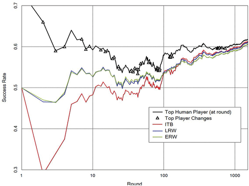
displays the results of the MUFTC game when quadratic scoring is used. The approximation of the top human player by the three meta-inductive methods becomes tighter. More importantly, the performance ordering between the three meta-inductive methods is reversed, compared to the natural scoring: ERW is now slightly better than that of LRW, which is in turn significantly better than ITB. These findings are in accordance with our theoretical results in sections 4 and 5, where we recognised that the avoidance of significant regrets is more rewarded under quadratic compared to linear scoring and that in this respect, ERW performs better than LRW, and LRW significantly better than ITB.

Figure 4. Application of meta-induction to the MUFTC with quadratic scoring (logarithmic time scale). ITB is lowest, followed by LRW, ERW and T.H.P.

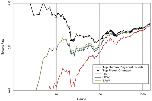
Our second real-world application is based on a pioneering psychological study of cue-based prediction tournaments: the twenty data sets presented in Czerlinski et al. (Citation1999), hereafter called the CGG Data Sets. Each of these data sets consists of information about a domain of real-world objects, eg, German cities, in regard to a criterion variable about these objects, eg, the size of the city (number of inhabitants). The data sets consist of binary cues (eg, whether the cities have a first division football club, whether they have a university, etc.) that are positively correlated with the criterion variable. The prediction task is to judge, on the basis of these cues, which of the two objects (eg, Bonn or Nürnberg) has the higher value of a given criterion variable.

For each of the CGG Data Sets, we generated 100 prediction games, with each game consisting of a sequence of 100 paired comparison tasks. Each task was determined by selecting two objects at random from the relevant data set. If the first object had a greater value for the criterion variable, then the event value was 1, and otherwise 0; there were no ties. For each of the prediction games, the cues represented in the data set were treated as the accessible base methods, where a cue predicts 1, if the first object has a higher cue value, predicts 0, if the second object has a higher cue, and predicts 0.5, otherwise. The participating meta-inductive methods were ITB, LRW, and ERW. presents the achieved success rates for the top cue, along with ITB, LRW, and ERW, for each of the 20 data sets. Although the cues with highest success rates are different in each domain, the success rates of the meta-inductive methods approximate them closely from below in each domain or even from above in the case of ERW and quadratic scoring. Under a natural scoring (middle column), the performance of the three meta-methods followed the order ITB, LRW, and ERW (apart from a few exceptions marked in blue/dark). This confirms the theoretical result in sections 4 and 5 that the minimisation of the worst case regret achieved by ERW and (less) by LRW comes at a certain short-run regret. The results change entirely if we apply a quadratic scoring (right column), by which the avoidance of high regrets is more rewarded. Now, ERW outperforms LRW and ITB for all 20 data sets, and even the top cue for 15 of the 20 data sets; moreover, LRW also outperforms ITB in 19 of the 20 data sets.

Table 12. Application of meta-induction to the CGG Data Sets. Left column: cues (base methods). Middle column: natural scoring (performance ranking Top Cue $>$ ITB $>$ LRW $>$ ERW; exceptions marked in blue/dark). Right column: quadratic scoring (performance ranking ERW $>$ Top Cue $>$ LRW $>$ ITB; exceptions marked in blue/dark).

Display Table

It is an important task for the future to investigate, along these lines, the performance of meta-inductive strategies in application to forecasting and planning algorithms over real-world problems, as developed more recently, for example, in J Wang et al. (Citation2020), Khan et al. (Citation2020), Y Wang et al. (Citation2021) and Bi et al. (Citation2021).

Code availability

Program code in Visual Basic available under

DOI: https://doi.org/10.5281/zenodo.5770223

Acknowledgments

For valuable help, we are indebted to Konstantinos Katsikopoulos, Ronald Ortner, Igor Douven, Tom Sterkenburg, Christian Feldbacher-Escamilla, Peter Brössel and Leah Henderson.

Disclosure statement

No potential conflict of interest was reported by the author(s).

Additional information

Funding

This work was supported by the DFG (Deutsche Forschungsgemeinschaft), SPP 1516.

Notes

1. Cf. Rao et al. (Citation1994), sec. 4, and Giraud-Carrier and Provost (Citation2006), sec. 3, who cite statements from a 1994 e-mail discussion in the Machine Learning List launched by Michael J. Pazzani (Machine Learning List 6, numbers 19–27).

2. Cf. Schurz (Citation2008, Citation2019), Schurz and Thorn (Citation2016, Citation2017), Thorn and Schurz (Citation2019), (Henderson, Citation2020, sec. 7.3), Sterkenburg (Citation2020, Citation2019), Feldbacher-Escamilla and Schurz (Citation2020), Douven (Citation2021).

3. New are the insights about ERW’s slower forgetting rate compared to LRW, the improved result about cRW, the discussion of Rao et al. (Citation1994), and partly definition 3, the proof of theorem 2, theorem 4, and .

4. In Schurz (Citation2008, Citation2019) regrets are called attractivities, since the regret of a method expresses its attractivity for the meta-inductivist.

5. For the proof, see Schurz (Citation2019), appendix 12.25. Note that theorem 6.11 in Schurz (Citation2019) states a worse bound for rRW, namely,

\frac{r - 1}{2 \cdot k}

instead of

\frac{r - 1}{k}

. However, the proof in Schurz (Citation2019) can easily be adapted to prove the better bound: on p. 154, ‘1’ has to be replaced by ‘0.5’ in lines 8, 11, 12 and 17, and on p 334, ‘one’ resp. ‘1’ has to be replaced by ‘0.5’ in lines 5 and 6, ‘

\leq

1’ by ‘

\leq

by 0.5’ in line 7, and ‘1/k’ by ‘1/2

\cdot

k’ in lines 15 and 17.

6. Wolpert assumes that prediction methods are computable, but this requirement is not strictly necessary.

7. Wolpert (Citation1996) mentions weakly homogeneous loss functions and the weak no-free lunch theorem in a small paragraph on p. 1354; for our purpose this version of Wolpert’s theorem is the most important.

8. Theorem 4 and its proof generalise to symmetrically distributed intervals of (uncountably many) values, if sums are replaced by integrals.

9. K(s) is defined as the length of the shortest program generating s, written in the language of a universal computer (K-measures obtained from different universal computers differ from each other by an additive constant). The definition generalises to infinite sequences by taking the limit of $K ((e_{1}, \dots, e_{n})) / n$ for $n \to \infty$ (cf. Staiger, Citation2007). The negative exponential of this limit complexity relates to the probability density of an infinite sequence (cf. Cover & Thomas, Citation1991, ch. 7). The qualitative explanation of this result is as follows: The farther the (limiting) frequency of a sequence is away from 1/2, the smaller its complexity and the fewer sequences exist that have this frequency (which is a consequence of the Binomial formula). Thus individual sequences with low complexity have a higher frequency-uniform probability than those with high complexity.

10. Program code available under DOI: https://doi.org/10.5281/zenodo.5770223

11. In Bayesianism these scoring functions are called ‘proper’ because using them maximises the expectation value of predictive success, provided one predicts the probabilities of events (instead of their truth values, in which case predictive success is maximised under linear scoring functions; cf. Gneiting and Raftery (Citation2007)).

12. https://probabilistic-footy.monash.edu/ $\sim$ footy/.

References

Bi, J., Yuan, H., Duanmu, S., Zhou, M., & Abusorrah, A. (2021). Energy-optimized partial computation offloading in mobile-edge computing with genetic simulated-annealing-based particle swarm optimization. IEEE Internet of Things Journal, 8(5), 3774–3785. https://doi.org/10.1109/JIOT.2020.3024223
Web of Science ®Google Scholar
Carnap, R. (1962). Logical Foundations of Probability (2nd edn ed.). University of Chicago Press.
Google Scholar
Cesa-Bianchi, N., & Lugosi, G. (2006). Prediction, Learning, and Games. Cambridge University Press.
Google Scholar
Cover, T., & Thomas, J. (1991). Elements of Information Theory. Wiley Interscience.
Google Scholar
Czerlinski, J., Gigerenzer, G., & Goldstein, D. G. (1999). How good are simple heuristics? In G. Gigerenzer & P. M. Todd, & the ABC Research Group (Eds.), Simple heuristics that make us smart (pp. 97–118). Oxford University Press.
Google Scholar
Douven, I. (2021). Explaining the success of induction. British Journal for the Philosophy of Science https://doi.org/10.1086/714796. forthcoming.
Web of Science ®Google Scholar
Feldbacher-Escamilla, C., & Schurz, G. (2020). Optimal probability aggregation based on generalized brier scoring. Annals of Mathematics and Artificial Intelligence, 88(7), 717–734. https://doi.org/10.1007/s10472-019-09648-4
Web of Science ®Google Scholar
Gigerenzer, G. , Todd, P.M. & the ABC Research Group. (1999). Simple heuristics that make us smart (& eds). Oxford University Press.
Google Scholar
Giraud-Carrier, C., & Provost, F. (2006) Toward a justification of meta-learning: Is the no free lunch theorem a show-stopper? In: Proceedings of the ICML-2005 Workshop on Meta-learning. 22nd international machine learning conference (ICML 205), pp 12–19.
Google Scholar
Gneiting, T., & Raftery, A. E. (2007). Strictly proper scoring rules, prediction, and estimation. Journal of the American Statistical Association, 102(477), 359–378. https://doi.org/10.1198/016214506000001437
Web of Science ®Google Scholar
Henderson, L. (2020). The problem of induction. In E. Zalta (Ed.), Stanford Encyclopedia of Philosophy (Spring 2020 Edition) https://plato.stanford.edu/archives/spr2020/entries/induction-problem
Google Scholar
Heys, W., & Winkler, R. (1970). Statistics: Probability, Inference, and Decision (Vol. 1). Holt.
Google Scholar
Howson, C., & Urbach, P. (1996). Scientific Reasoning: The Bayesian Approach (2nd edn ed.). Open Court.
Google Scholar
Khan, A., Cao, Z., Li, S., Katsikis, V., & Liao, L. (2020). BAS-ADAM: An ADAM based approach to improve the performance of beetle antennae search optimizer. IEEE/CAA Journal of Automatica Sinica, 7(2), 461–471. https://doi.org/10.1109/JAS.2020.1003048
Google Scholar
Lemke, C., Budka, M., & Gabrys, B. (2015). Meta-learning: A survey of trends and technologies. Artificial Intelligence Review, 44, 117–130 https://link.springer.com/article/10.1007/s10462-013-9406-y.
PubMed Web of Science ®Google Scholar
Mourtada, J., & Maillard, O. A. (2017). Efficient tracking of a growing number of experts. Proceedings of Machine Learning Research, 76, 1–23 https://proceedings.mlr.press/v76/mourtada17a/mourtada17a.pdf.
Google Scholar
Rao, R., Gordon, D., & Spears, W. (1994). For every generalization action, is there really an equal and opposite reaction? In: Machine Learning (Proceedings of ICML 1995), Burlington/MA: Morgan Kaufmann, pp 471–479.
Google Scholar
Salmon, W. (1957). Should we attempt to justify induction? Philosophical Studies, 8(3), 45–47. https://doi.org/10.1007/BF02308902
Web of Science ®Google Scholar
Schaffer, C. (1994) A conservation law for generalization performance. In: Machine Learning (Proceedings of ICML 1994), Burlington/MA: Morgan Kaufmann, pp 259–265.
Google Scholar
Schurz, G. (2008). The meta-inductivist’s winning strategy in the prediction game: A new approach to Hume’s problem. Philosophy of Science, 75 (3) , 278–305. https://doi.org/10.1086/592550
Web of Science ®Google Scholar
Schurz, G., & Thorn, P. (2016). The revenge of ecological rationality: Strategy- selection by meta-induction. Minds and Machines, 26(1), 31–59. https://doi.org/10.1007/s11023-015-9369-7
Web of Science ®Google Scholar
Schurz, G., & Thorn, P. (2017). A priori advantages of meta-induction and the no free lunch theorem: A contradiction? In G. Kern-Isberner, J. Fűrnkranz, & M. Thimm (Eds.), KI 2017: Advances in Artificial Intelligence (Lecture Notes in Computer Science (Vol. 10505, pp. 236–248). Springer.
Google Scholar
Schurz, G. (2019). Hume’s Problem Solved: The optimality of meta-induction. MIT Press.
Google Scholar
Shalev-Shwartz, S., & Ben-David, S. (2014). Understanding Machine Learning. From Theory to Algorithms. Cambridge University Press.
Google Scholar
Solomonoff, R. (1964). A formal theory of inductive inference. Information and Control, 7(1), 1–22, 224–254. https://doi.org/10.1016/S0019-9958(64)90223-2
Google Scholar
Staiger, L. (2007). The Kolmogorov complexity of infinite words. Theoretical Computer Science, 383(2–3), 187–199. https://doi.org/10.1016/j.tcs.2007.04.013
Web of Science ®Google Scholar
Sterkenburg, T. (2019). The meta-inductive justification of induction: The pool of strategies. Philosophy of Science, 86(5), 981–992. https://doi.org/10.1086/705526
Web of Science ®Google Scholar
Sterkenburg, T. (2020). The meta-inductive justification of induction. Episteme, 7(4), 519–541. https://doi.org/10.1017/epi.2018.52
Google Scholar
Thorn, P., & Schurz, G. (2019). Meta-inductive prediction based on attractivity weighting: An empirical performance evaluation. Journal of Mathematical Psychology, 89, 13–30. https://doi.org/10.1016/j.jmp.2018.12.006
Web of Science ®Google Scholar
Wang, J., Sun, Y., Zhang, Z., & Gao, S. (2020). Solving multitrip pickup and delivery problem with time windows and manpower planning using multiobjective algorithms. IEEE/CAA Journal of Automatica Sinica, 7(4), 1134–1153. https://doi.org/10.1109/JAS.2020.1003204
Google Scholar
Wang, Y., Gao, S., Zhou, M., & Yu, Y. (2021). A multi-layered gravitational search algorithm for function optimization and real-world problems. IEEE/CAA Journal of Automatica Sinica, 8(1), 94–109. https://doi.org/10.1109/JAS.2020.1003462
Google Scholar
Wolpert, D. (1992). On the connection between in-sample testing and generalization error. Complex Systems, 6 (1) , 47–94. https://www.complex-systems.com/abstracts/v06_i01_a05/.
Google Scholar
Wolpert, D., & Macready, W. (1995) No free lunch theorems for search. Tech. Rep. Technical Report SFI-TR-95-02-010, Santa Fe Institute.
Google Scholar
Wolpert, D. (1996). The lack of a priori distinctions between learning algorithms. Neural Computation, 8(7), 1341–1390. https://doi.org/10.1162/neco.1996.8.7.1341
Web of Science ®Google Scholar

Escaping the No Free Lunch Theorem: A Priori Advantages of Regret-Based Meta-Induction

ABSTRACT

1. Introduction: the NFL theorem and Hume’s problem of induction

Table 2. Meta-induction and no-free lunch for binary event games. Effect of the increase of rounds from 10 to 20 for M-I, M-AI, LRW, and ERW. Cells show the percentages of sequences in which success rates within respective intervals (left margin) have been reached.

Table 4. Meta-induction for binary events from the perspective of a frequency-uniform distribution. Cells show (average) absolute successes of the six methods M-I, M-AI, Av, ITB, LRW, and ERW, for binary sequences with 20 rounds, depending on their event frequencies (left margin).

2. Regret-weighted meta-induction

3. NFL theorems for prediction games

4. Meta-induction and NFL in the long-run perspective

5. Meta-induction and NFL in the short-run perspective: binary events

6. Meta-induction and NFL in the short-run perspective: real-valued events

Table 11. Meta-induction over real-valued event sequences dependent on their entropy. Cells display the average absolute successes of the listed methods over all possible sequences of 20 rounds with three asymmetrically distributed possible events 0.1, 0.2 and 0.9, depending on entropy.

Conclusion and outlook

Code availability

Acknowledgments

Disclosure statement

References

Information for

Open access

Opportunities

Help and information

Escaping the No Free Lunch Theorem: A Priori Advantages of Regret-Based Meta-Induction

ABSTRACT

1. Introduction: the NFL theorem and Hume’s problem of induction

Table 2. Meta-induction and no-free lunch for binary event games. Effect of the increase of rounds from 10 to 20 for M-I, M-AI, LRW, and ERW. Cells show the percentages of sequences in which success rates within respective intervals (left margin) have been reached.

Table 4. Meta-induction for binary events from the perspective of a frequency-uniform distribution. Cells show (average) absolute successes of the six methods M-I, M-AI, Av, ITB, LRW, and ERW, for binary sequences with 20 rounds, depending on their event frequencies (left margin).

2. Regret-weighted meta-induction

3. NFL theorems for prediction games

4. Meta-induction and NFL in the long-run perspective

5. Meta-induction and NFL in the short-run perspective: binary events

6. Meta-induction and NFL in the short-run perspective: real-valued events

Table 11. Meta-induction over real-valued event sequences dependent on their entropy. Cells display the average absolute successes of the listed methods over all possible sequences of 20 rounds with three asymmetrically distributed possible events 0.1, 0.2 and 0.9, depending on entropy.

Conclusion and outlook

Code availability

Acknowledgments

Disclosure statement

Additional information

Funding

Notes

References

Related research

To cite this article:

Download citation

Your download is now in progress and you may close this window

Login or register to access this feature

Information for

Open access

Opportunities

Help and information

Keep up to date