Bridging macroeconomic data between statistical classifications: the count-seed RAS approach

ABSTRACT

In applications, it is often necessary to link heavily aggregated macroeconomic datasets adhering to different statistical classifications. We propose a simple data reclassification procedure for those cases in which a bridge matrix grounded in microdata is not available. The essential requirement of our approach, which we refer to as count-seed RAS, is that there exists a time period or a geographical entity similar to the one of interest for which the relevant economic variable is observed according to both classifications. From this information, a bridge matrix is constructed using bi-proportional methods to rescale a seed matrix based on a qualitative correspondence table from official sources. We test the procedure in two case studies and by Monte Carlo methods. We find that, in terms of reclassification accuracy, it performs noticeably better than other expeditious methods. The analytical framework underlying our approach may prove a useful way of conceptualizing data reclassification problems.

KEYWORDS:

• Classification change
• data reclassification
• bridge matrix
• conversion factors
• backcasting

1. Introduction

In applied research and policy analysis work, it often becomes necessary to link heavily aggregated macroeconomic datasets that adhere to different statistical classifications. Most commonly, this occurs as a result of the revisions that industry and product classifications are periodically subjected to. In the late 2000s, for example, the national accounts of European Union member states switched from revision 1.1 to revision 2 of the ‘Statistical classification of economic activities in the European Community’ (NACE, from the French acronym). When the boundaries of an industry shift, comparability over time is lost for important economic variables such as value added or employment. Then, obtaining consistent time series for the industry-level variables of interest requires conversion between classifications. In addition, reclassification is often unavoidable when using timely data with existing policy analysis models. Indeed, because calibration is a complex and time-consuming endeavor, macroeconomic models can remain anchored to outdated data structures long after a new classification has been adopted.

Classification revisions, however, are not the only reason why the need for data conversion may arise. Sometimes one needs to combine datasets that are natively collected on the basis of different classifications. Consider data on final use by households. In the Supply and Use Framework (Eurostat, 2008; United Nations Statistical Commission, 2009), each transaction is categorized according to the characteristics of the good or service that is being exchanged. In a European context, this means that data on final use by households have to be organized according to the ‘Statistical Classification of Products by Activity’ (CPA). Household surveys, however, typically collect information about the purpose for which expenditures are made, and not about the type of goods or services that are being acquired. These surveys usually adopt the ‘Classification of individual consumption by purpose’ (COICOP). Before the data can be incorporated in the IO framework, they must undergo conversion from COICOP to CPA (Kronenberg, 2011). This kind of reclassification problem emerges frequently in macroeconomic policy analysis models (Capros et al., 2013; Kratena et al., 2017).

In the context of their institutional activities, national statistical institutes routinely construct conversion factors that allow bridging data between classifications. Consider, for example, what happens when a revision of the industry classification takes place. In principle, historical records could be re-expressed in the new classification by recoding each individual observation in the microdata. This approach is costly and not always feasible, so it is only applied to short time periods, if at all. Most commonly, existing datasets are converted on the basis of proportional mappings between aggregates of the two classifications. Such mappings – variously called concordances, conversion factors, or bridge matrices – are constructed from cross-tabulations of dual-coded data. The process is referred to as backcasting. Smith and James (2017) offer an interesting account of how the most recent industry classification change was handled in the UK Yuskavage (2007) documents US experiences.

Conversion factors, however, are not typically released to the public. Even when they are (Drew and Dunn, 2011; ONS, 2017), it is rarely the case that the degree of aggregation is aligned to the needs of the analyst. In practice, when it comes to classification issues, independent researchers are generally left to their own devices. To the best of the authors’ knowledge, the academic literature provides little guidance as to how to handle data reclassification problems. Like other common data management tasks, classification issues are rarely discussed (see Lenzen et al., 2012; Rueda-Cantuche et al., 2013, for exceptions). The few studies of bridge matrices that could be located have not appeared in peer-reviewed publications (e.g. Kronenberg, 2011; Perani and Cirillo, 2015). By and large, it appears that in applied work practitioners predominantly use expert judgment to establish best-guess correspondences between aggregates of the source and target classifications. The process of specifying such correspondence is often tedious and its outcome somewhat subjective.

This paper describes a simple, mechanical and reproducible approach to the construction of bridge matrices under conditions of data availability that are likely to be met in most circumstances. From a practical standpoint, the essential requirement is that there exists an earlier or later time period – or a geographical area that is similar enough to the one of interest – for which the relevant economic variable can be observed in both the source and the target classification. Using this information, we estimate a contingency table that links the two classifications by means of bi-proportional scaling methods. Finally, data reclassification is carried out using conversion factors computed from that table.

Estimating an unknown matrix by proportionally scaling an initial guess – typically referred to as the seed or prior matrix – using known marginal totals is a routine practice in a variety of fields (Idel, 2016; Lomax and Norman, 2016). In input–output economics, the procedure is known as RAS (Lahr and De Mesnard, 2004; Miller and Blair, 2009). What is challenging about the specific RAS application discussed here is that it is not obvious how to construct a plausible seed matrix. In the spirit of Lenzen et al. (2012) and Lenzen and Lundie (2012), a simple option would be to use a binary seed matrix based on a readily available qualitative table of correspondences between classifications. All data reclassifications in Cai (2016), for example, took this approach. In fact, we argue that from the very same table of correspondences a more informative prior matrix can be constructed just as easily. In a nutshell, the proposed seed matrix is compiled by counting the number of fundamental items (i.e. items defined at the most disaggregated level of the classification) that simultaneously contribute to a given pair of source- and target-classification aggregates. We refer to the data reclassification procedure we propose as count-seed RAS.

We assess the performance of count-seed RAS reclassification in two case studies for which the conversion factors used by the statistical office are known. We then examine the procedure in a more general context using Monte Carlo methods. In spite of its simplicity, we find that the count-seed RAS approach yields encouraging results. In a broader sense, we argue that the analytical framework described in this paper provides a useful way of conceptualizing data reclassification problems.

2. Methodological framework

2.1. The data reclassification problem

Consider a nonnegative $n\times 1$ vector, $\mathbf{\text{x}}$, whose elements describe the value of a certain economic variable of interest to a very fine degree of disaggregation. We refer to $\mathbf{\text{x}}$ as the ‘fundamental’ vector. Conceivably, the fundamental vector could be observed, but – for reasons that range from the nature of the estimation procedures to considerations of reliability and confidentiality – the statistical office only releases the information in the form of a much more coarsely aggregated vector, say, $\mathbf{\text{y}}$. The relationship between $\mathbf{\text{x}}$ and $\mathbf{\text{y}}$ can be formalized as $\mathbf{\text{y}}=\mathbf{\text{Sx}}$ where $\mathbf{\text{S}}$ represents an $m\times n$ aggregation matrix. By calling it an aggregation matrix, we mean that: (a) $\mathbf{\text{S}}$ has much fewer rows than columns, i.e. $m\ll n$, and; (b) because aggregation is exhaustive and mutually exclusive, all of the elements in any given column of $\mathbf{\text{S}}$ are zero, except for one element which is equal to one. In other words, ${\mathbf{\text{i}}}_m^{\mathrm{\top }}\mathbf{\text{S}}={\mathbf{\text{i}}}_n^{\mathrm{\top }}$, where the symbol ${\mathbf{\text{i}}}_p$ resents a column vector of ones with length $p$. Conversely, summing along a generic row of $\mathbf{\text{S}}$ yields the count of how many elements of $\mathbf{\text{x}}$ are aggregated together into the corresponding element of $\mathbf{\text{y}}$. For example, an aggregation matrix $\mathbf{\text{S}}$ with the following structure $\left(\begin{array}{cccccccccc}1& 1& 1& 0& 0& 0& 0& 0& 0& 0\\ 0& 0& 0& 1& 0& 0& 0& 0& 0& 0\\ 0& 0& 0& 0& 1& 1& 0& 0& 0& 0\\ 0& 0& 0& 0& 0& 0& 1& 1& 1& 1\end{array}\right)$ aggregates a vector $\mathbf{\text{x}}$ of length 10 into a vector $\mathbf{\text{y}}$ of length 4. It does so by respectively summing together the elements in positions 1–3, 5–6 and 7–10 of $\mathbf{\text{x}}$, while leaving element 4 unaffected.

The problem of converting economic data between classifications can be framed as follows. Consider two distinct aggregations of the unobserved fundamental vector. Respectively, the two aggregation matrices are denoted ${\mathbf{\text{S}}}_1$ and ${\mathbf{\text{S}}}_2$, consist of $m_1$ and $m_2$ aggregates and yield aggregate vectors ${\mathbf{\text{y}}}_1={\mathbf{\text{S}}}_1\mathbf{\text{x}}$ and ${\mathbf{\text{y}}}_2={\mathbf{\text{S}}}_2\mathbf{\text{x}}$. The analyst needs information about ${\mathbf{\text{y}}}_2$, but can only observe ${\mathbf{\text{y}}}_1$. The aggregation matrices, on the other hand, are both known.

Throughout the paper, ${\mathbf{\text{S}}}_1$ is and ${\mathbf{\text{S}}}_2$ are referred to as the ‘source’ and ‘target’ classification, respectively. Correspondingly, ${\mathbf{\text{y}}}_1$ and ${\mathbf{\text{y}}}_2$ are designated as the source and the target vector. For ease of exposition, the remainder of this section assumes that the economic variable at the center of the analysis is gross output and that what makes reclassification necessary is a revision of the industry classification underlying the national accounting system. Even so, the framework is general enough to apply to a number of data reclassification problems that arise frequently in applied work.

In what follows, the aggregation matrices are thought of as adding together ‘products’ (corresponding to the elements of $\mathbf{\text{x}}$) to form ‘industries’ (corresponding to the elements of ${\mathbf{\text{y}}}_1$ and ${\mathbf{\text{y}}}_2$). We emphasize that, in the context of our methodological discussion, the terms ‘product’ and ‘industry’ are merely used as convenient shorthand for the entries of vectors with different degrees of aggregation. In other words, our terminology does not make any reference to the notion of product and industry adopted for the purpose of national accounting.

2.2. Bridge matrices and conversion factors

In the production of official statistics, such data reclassification problems are typically overcome using an existing contingency table in which the economic variable of interest is cross-tabulated according to the two classifications. Let $\mathbf{\text{C}}$ be the $m_1\times m_2$ contingency table linking the source and the target classification. A generic element $c_{ij}$ of $\mathbf{\text{C}}$ represents the value of gross output that is classified as an output of industry $i$ under the source classification and as an output of industry $j$ under the target classification. Clearly, if $\mathbf{\text{C}}$ itself were known, the reclassification problem would be trivial, as ${\mathbf{\text{y}}}_1$ and ${\mathbf{\text{y}}}_2$ would simply emerge from adding up along the rows and columns of $\mathbf{\text{C}}$, respectively (i.e. $\mathbf{\text{C}}{\mathbf{\text{i}}}_{m_2}={\mathbf{\text{y}}}_1$ and ${\mathbf{\text{i}}}_{m_1}^{\mathrm{\top }}\mathbf{\text{C}}={\mathbf{\text{y}}}_2^{\mathrm{\top }}$). Instead, what might be available in practice is a surrogate contingency table, ${\mathbf{\text{C}}}^{\mathbf{\text{o}}}$, relating to a different time period or geographical area. For example, when the industry classification at the basis of the national accounts is revised, there is generally a transition period during which data collection at the unit level is typically carried out using both the new and the old classification. Cross-tabulation of such dual-coded microdata yields a contingency table that can be used as the basis for reclassification in different years. The surrogate contingency table ${\mathbf{\text{C}}}^{\mathbf{\text{o}}}$ is henceforth referred to as the ‘base-year’ contingency table.

From ${\mathbf{\text{C}}}^{\mathbf{\text{o}}}$, a so-called bridge matrix is straightforwardly obtained as (1) ${\mathbf{\text{B}}}^{\mathbf{\text{o}}}=({\widehat{\mathbf{\text{y}}}}_1^{\mathbf{\text{o}}}{)}^{-1}{\mathbf{\text{C}}}^{\mathbf{\text{o}}}$(1) with ${\mathbf{\text{y}}}_1^{\mathbf{\text{o}}}={\mathbf{\text{C}}}^{\mathbf{\text{o}}}{\mathbf{\text{i}}}_{m_2}$. A superimposed hat denotes diagonalization of a vector into a square matrix. A generic entry of ${\mathbf{\text{B}}}^{\mathbf{\text{o}}}$ takes the form $b_{ij}^{\mathrm{o}}=c_{ij}^{\mathrm{o}}/\sum _{k=1}^{m_2}{c}_{ik}^{\mathrm{o}}$. The elements of ${\mathbf{\text{B}}}^{\mathbf{\text{o}}}$ are often termed conversion factors. A conversion factor $b_{ij}^{\mathrm{o}}$ can be interpreted as an estimate of the conditional probability of an item being reassigned to the $j$-th industry of the target classification given that it accrued the $i$-th industry under the source classification.

Given the bridge matrix ${\mathbf{\text{B}}}^{\mathbf{\text{o}}}$, an estimate of ${\mathbf{\text{y}}}_2$ is computed as (2) ${\mathbf{\text{y}}}_2^{\ast \mathrm{\top }}={\mathbf{\text{y}}}_1^{\mathrm{\top }}{\mathbf{\text{B}}}^{\mathbf{\text{o}}}$(2)

2.3. Bridge matrices under limited data availability

In general, the ${\mathbf{\text{C}}}^{\mathbf{\text{o}}}$ (levels) and ${\mathbf{\text{B}}}^{\mathbf{\text{o}}}$ (conversion factors) matrices that statistical offices use in their institutional activities are not readily available to independent researchers. Whenever conversion factors cannot be obtained from official sources, analysts have to develop their own approach to data reclassification.

If an estimate, say, ${\widetilde{\mathbf{\text{C}}}}^{\mathbf{\text{o}}}$ of the base-year contingency table were available, a natural way to proceed would be to compute a bridge matrix from that estimate, (3) ${\widetilde{\mathbf{\text{B}}}}^{\mathbf{\text{o}}}={\widehat{\mathbf{\text{r}}}}^{-1}{\widetilde{\mathbf{\text{C}}}}^{\mathbf{\text{o}}}$(3) where $\mathbf{\text{r}}={\widetilde{\mathbf{\text{C}}}}^{\mathbf{\text{o}}}{\mathbf{\text{i}}}_{m_2}$ represents the row totals of ${\widetilde{\mathbf{\text{C}}}}^{\mathbf{\text{o}}}$. Then, the reclassified output vector would be estimated as (4) ${\widetilde{\mathbf{\text{y}}}}_2^{\ast \mathrm{\top }}={\mathbf{\text{y}}}_1^{\mathrm{\top }}{\widetilde{\mathbf{\text{B}}}}^{\mathbf{\text{o}}}$(4) A vector that takes the form (4) will be henceforth referred to as a reclassification of ${\mathbf{\text{y}}}_1$ or simply as a ‘reclassified vector’. A reclassified vector such as (2) – which is computed on the basis of ${\mathbf{\text{C}}}^{\mathbf{\text{o}}}$ itself, as opposed to an estimate thereof – is designated as a ‘benchmark vector’.

How is the base-year contingency table to be estimated in applied work? In this respect, it is useful to note that very often, even though ${\mathbf{\text{C}}}^{\mathbf{\text{o}}}$ itself is unobserved, its row and column totals are known. For example, when a new industry classification is adopted, there is typically at least one year for which the statistical office will report all key economic variables according to both the old and the new standard. If this is the case, one may attempt to estimate the base-year contingency table using the RAS algorithm.

In IO applications, RAS is a very popular approach to the estimation of a matrix from its row and column totals (Lahr and De Mesnard, 2004; Miller and Blair, 2009). The algorithm is initialized with a preliminary estimate of the matrix of interest. Iteratively, the entries of that matrix are proportionally rescaled to the required marginal totals, alternating between row- and column-wise adjustments. Convergence is declared when all adding up constraints on the rows and columns of the matrix are simultaneously satisfied.

Implementing this approach in our context requires that a seed matrix reflecting prior knowledge of ${\mathbf{\text{C}}}^{\mathbf{\text{o}}}$ be specified. In this respect, it is important to note that the scaled matrix emerging from RAS is known to be quite sensitive to the choice of the starting values. Thus, serious misspecification of the seed matrix may result in a misleading contingency table estimate. At least under favorable conditions, however, there are reasons to believe that – even if the seed matrix is fairly inaccurate – the reclassification obtained from a RAS-based bridge matrix may not depart dramatically from the benchmark reclassification (2). To see why this is the case, consider the following heuristic argument. Suppose that the row and column totals of the estimated contingency table ${\widetilde{\mathbf{\text{C}}}}^{\mathbf{\text{o}}}$ match those of the base-year table ${\mathbf{\text{C}}}^{\mathbf{\text{o}}}$. This is true by construction of any RAS-based estimate. It follows trivially from (3) and (4) that, irrespective of the interior of the matrix, the conversion factors obtained from ${\widetilde{\mathbf{\text{C}}}}^{\mathbf{\text{o}}}$ reproduce the benchmark reclassification exactly in the base year (i.e. for ${\mathbf{\text{y}}}_1={\mathbf{\text{y}}}_1^{\mathbf{\text{o}}}$). Now consider what happens as you move away from the base year. Suppose for a moment that over time all the elements of the source vector change at exactly the same rate. Under these circumstances, the entries of the reclassified vector also evolve at that very same constant rate, regardless of what bridge matrix is used in (4). In this special case, then, any two distinct bridge matrices that produce identical reclassifications in the base year would also produce identical reclassifications in other time periods. Specifically, any RAS-based bridge matrix – irrespective of the underlying seed – would replicate the benchmark reclassification (i.e. ${\widetilde{\mathbf{\text{y}}}}_2^{\ast }={\mathbf{\text{y}}}_2^{\ast }$) in each period. In practice, the various elements of the source vector will grow at different rates over time. Even so, as long as those rates only exhibit moderate diversity, it seems unlikely that a reclassification produced by RAS-based methods would lie very far from the benchmark reclassification in time periods that are reasonably close to the base year.

2.4. Seed matrix specification

How can a seed matrix that is both informative and feasible be obtained in an applied context? Work on the construction of semi-survey enterprise input–output tables by Lenzen and Lundie (2012) suggests that, in the absence of more precise prior information, a fairly sparse non-negative matrix can still be recovered to a reasonable degree of accuracy by initializing RAS with a binary matrix that identifies which elements of the estimated are believed to be nonzero. In our context, a correctly specified binary seed in the spirit of Lenzen and Lundie (2012) would be given by an $m_1\times m_2$ matrix, ${\mathbf{\text{D}}}^{\mathbf{\text{b}}}$, whose generic element $d_{ij}^b$ is one if source industry $i$ and target industry $j$ have at least one fundamental product in common, and zero otherwise. For example, this is the form taken by the ‘concordance matrices’ that link classifications over time in Lenzen et al. (2012). Data reclassification based on RAS-ing ${\mathbf{\text{D}}}^{\mathbf{\text{b}}}$ with the marginal totals of ${\mathbf{\text{C}}}^{\mathbf{\text{o}}}$ is henceforth referred to as the ‘binary-seed RAS’ approach. Note that, because ${\mathbf{\text{D}}}^{\mathbf{\text{b}}}$ is nonnegative and has the same pattern of zeros as ${\mathbf{\text{C}}}^{\mathbf{\text{o}}}$, the balancing problem underlying binary-seed RAS reclassification is well behaved (Idel, 2016).

We argue that a closely related approach based on an alternative seed matrix specification will generally perform better than binary-seed RAS. Notice that the contingency matrix that we aim to estimate can be written as (5) ${\mathbf{\text{C}}}^{\mathbf{\text{o}}}={\mathbf{\text{S}}}_1{\widehat{\mathbf{\text{x}}}}^{\mathbf{\text{o}}}{\mathbf{\text{S}}}_2^{\mathrm{\top }}$(5) where ${\mathbf{\text{x}}}^{\mathbf{\text{o}}}$ denotes the value of the fundamental vector in the base year. Because in applications virtually nothing is known about the elements of ${\mathbf{\text{x}}}^{\mathbf{\text{o}}}$, we postulate that they are each an independent draw from some unspecified distribution with mean $\mu >0$. Then, $\text{E}\left({\mathbf{\text{x}}}^{\mathbf{\text{o}}}\right)=\mu {\mathbf{\text{i}}}_n$ and (6) $\text{E}\left({\mathbf{\text{C}}}^{\mathbf{\text{o}}}\right)=\mu \mathbf{\text{D}}$(6) with $\mathbf{\text{D}}={\mathbf{\text{S}}}_1{\mathbf{\text{S}}}_2^{\mathrm{\top }}$. Based on this simple argument, we propose using $\mathbf{\text{D}}$ as the seed matrix for RAS. In this respect, the parameter $\mu$ that appears in (6) is merely a multiplicative factor whose value does not affect the outcome of bi-proportional scaling. Note that a generic element $d_{ij}$ of $\mathbf{\text{D}}$ is a count of the number of elements of the fundamental vector that are concurrently allocated to industry $i$ under the source classification and to industry $j$ under the target classification. Accordingly, RAS-based data reclassification that uses $\mathbf{\text{D}}$ as the prior matrix is termed ‘count-seed RAS’. Just like its binary-seed relative, the count-seed RAS approach results by construction in a well-behaved balancing problem.

In applications, $\mathbf{\text{D}}$ (as well as ${\mathbf{\text{D}}}^{\mathbf{\text{b}}}$) is easily compiled from a qualitative table of correspondences between the source and the target classifications. For a variety of statistical classifications, such correspondence tables can be retrieved from the United Nation's classification registry (http://unstats.un.org/unsd/cr/registry) and Eurostat's metadata center (http://ec.europa.eu/eurostat/ramon).

From a practical point of view, implementation of count-seed RAS reclassification consists of the following steps:

1. Obtain gross output data with the desired industry resolution in both the source (e.g. ISIC Rev.3 or NACE Rev.1.1) and the target classification (ISIC Rev.4 or NACE Rev.2);

2. Construct the seed matrix $\mathbf{\text{D}}$ by way of a simple cross-tabulation from the appropriate table of qualitative correspondences;

3. Scale the seed matrix to the required row and column totals using the RAS algorithm;

4. Compute the conversion factors from the resulting contingency table estimate and reclassify the data of interest.

Section 3 demonstrates this approach through a simple numerical example.

2.5. Validation

In an attempt to validate the count-seed RAS approach to data reclassification, Sections 4 and 5 examine its performance in the context of two case studies for which official conversion factors are available to the author, as well as by means of Monte Carlo simulations. All analyses are carried out in the R environment for statistical computing (R Core team, 2016). All data and scripts are available upon request from the authors.

At a basic level, we investigate whether the degree of inaccuracy associated with the count-seed RAS method lies within a range that would be generally deemed tolerable in policy analysis work. We then assess the method's performance in relation to three alternative and correspondingly simple approaches.

The first alternative we consider is probably the most widespread approach to data reclassification in applications. We refer to it as the ‘best-guess’ approach. By best-guess reclassification we mean the analysts’ practice of building bridge matrices by establishing plausible correspondences between the industries of the source and the target classification based on a qualitative description of the aggregates and on their own professional experience. It is in this relative and subjective sense that the word ‘best’ is to be understood in this context.

Secondly, we contrast the performance of count-seed RAS with that of binary-seed RAS. In this way, we aim to evaluate to what extent, if at all, reclassification accuracy is improved by adopting the seed matrix specification $\mathbf{\text{D}}$ put forward in this paper instead of a binary prior in the spirit of Lenzen and Lundie (2012), such as ${\mathbf{\text{D}}}^{\mathbf{\text{b}}}$.

Finally, we consider a ‘naive’ approach to reclassification based on the assumption that the economy produces exactly the same amount of each fundamental product. Specifically, the naive contingency estimate of ${\mathbf{\text{C}}}^{\mathbf{\text{o}}}$ is computed as ${\overline{x}}^{\mathrm{o}}\mathbf{\text{D}}$, with ${\overline{x}}^{\mathrm{o}}=n^{-1}\sum _i{x}_i^{\mathrm{o}}$. This represents the empirical equivalent of (5). In this sense, the error measures associated with the naive reclassification reflect the degree of inaccuracy of the prior information used as the starting point for count-seed RAS.

Each of these approaches is assessed in terms of: (a) how closely it recovers the true contingency table (‘estimation accuracy’), and; (b) how accurately it converts the source data to the target classification (‘reclassification accuracy’). To evaluate estimation accuracy, the same matrix dissimilarity metrics are employed as in Jackson and Murray (2004). Thus, estimation error is measured using Theil's U statistic, the weighted absolute difference (WAD), and the standardized total percentage error (STPE). Reclassification accuracy, on the other hand, is assessed through element-by-element comparisons between the reclassified vector ${\widetilde{\mathbf{\text{y}}}}_2^{\ast }$ and the target vector ${\mathbf{\text{y}}}_2$. From this perspective, the percentage error between corresponding entries of those two vectors represents a natural industry-level measure of reclassification error. It will often be convenient to summarize a vector of industry-specific PEs into a single scalar. For this purpose, we use the mean absolute percentage error (MAPE). When appropriate, we also report the 90th percentile of the distribution of the absolute percentage error (APE90) over industries. This quantity gives a sense of how significant the reclassification error can be for the most problematic industries. Formal definitions of all the error measures used in the paper can be found in Appendix A (online supplemental material).

Finally, a word of caution should be given regarding the quantification of the reclassification error in the case study analysis of Section 4. Contrary to what happens in a Monte Carlo setting – in which all elements of the reclassification problem are known – the target vector is intrinsically unobservable in real-world applications. Thus, in the case studies the reclassification error associated with ${\widetilde{\mathbf{\text{y}}}}_2^{\ast }$ is assessed relative to the benchmark reclassification ${\mathbf{\text{y}}}_2^{\ast }$. In other words, what is effectively being examined in the case studies is a method's ability to replicate the data reclassification that the statistical office would produce.

3. A simple numerical example

Consider a country whose output consists of the 15 fundamental products listed in the leftmost column of Table 1. The economy's gross output of each product in the base year is displayed in column 2. In the notation of Section 2, this corresponds to ${\mathbf{\text{x}}}^{\mathbf{\text{o}}}$. For the purpose of producing and reporting official data, the statistical office collapses the fundamental products into three broad industries: Agriculture, Manufacturing, and Services. Researchers outside the statistical office have access to industry output data, but not to the underlying product output data. Suppose that at some point in time the definition of the three industries in terms of the fundamental products is modified. In Table 1, columns 3 and 4 describe how products are assigned to industries in the source and in the target classification, respectively. The products affected by the change are shaded in gray. That the two classifications consist of the same number of identically named industries is only a simplification introduced for illustrative purposes.

TABLE 1. Alternative aggregations of the fundamental output vector.

Given the information in Table 1, moving from the source to the target definitions of Agriculture, Manufacturing and Services is merely a matter of adding together the fundamental gross output data according to a different aggregation scheme. One way of thinking about this reclassification exercise is in terms of a two-way table (Table 2). The main block of Table 2 represents the base-year contingency matrix ${\mathbf{\text{C}}}^{\mathbf{\text{o}}}$. The elements along the diagonal of ${\mathbf{\text{C}}}^{\mathbf{\text{o}}}$ can be thought of as referring to fundamental products that are assigned to the same aggregate under both classifications. Conversely, the off-diagonal elements account for products that the classification change shifts from one aggregate to another. Summing along the rows of the matrix yields output by aggregate according to the source classification. Summing along columns gives the output breakdown according to the target classification.

TABLE 2. Cross-tabulation of gross output by source and target classification.

		Target aggregates
		Agriculture	Manufacturing	Services	Total
	Agriculture	16	3	1	20
	Manufacturing	0	45	5	50
Source aggregates
	Services	0	0	30	30
	Total	16	48	36	100

Even inside the statistical office, fundamental dual-coded data of the kind underlying Tables 1 and 2 would not be available in the years preceding the classification change. Besides, the production of dual-coded data would only extend over a limited period of time – say, the base year – after which only the target classification would be used. For years other than the base year, data reclassification would be carried out using conversion factors obtained from the base-year contingency table.

Suppose, for instance, that the industry output data for an earlier year have to be backcast from the source into the target classification. Let the output of Agriculture, Manufacturing and Services in that earlier year be spelled out by the source vector ${\mathbf{\text{y}}}_1=(50,30,10{)}^{\mathrm{\top }}$. Using the bridge matrix implicit in Table 2, the benchmark vector would be computed as in Equation (2): ${\mathbf{\text{y}}}_2^{\ast \mathrm{\top }}=\left(\begin{array}{ccc}50& 30& 10\end{array}\right)\left(\begin{array}{ccc}.80& .15& .05\\ 0& .90& .10\\ 0& 0& 1\end{array}\right)=\left(\begin{array}{ccc}40& 34.5& 15.5\end{array}\right)$ Note that ${\mathbf{\text{y}}}_2^{\ast }$ is itself an estimate of the true target vector ${\mathbf{\text{y}}}_2$, which is unknown.

Now consider a researcher without access to the bridge matrix developed by the statistical office (let alone to the underlying contingency table). We propose replacing the unobserved base-year contingency table ${\mathbf{\text{C}}}^{\mathbf{\text{o}}}$ (Table 2) with an estimate constructed from the following two pieces of information: (1) a qualitative correspondence table specifying how the fundamental products are assigned to aggregates under the two classifications (i.e. Table 1 with column 2 suppressed); (2) gross output data for the base year both in the source and in the target classification (i.e. the row and column totals of ${\mathbf{\text{C}}}^{\mathbf{\text{o}}}$).

Given the product correspondences in Table 1, the seed matrix $\mathbf{\text{D}}$ is easily obtained by cross-tabulating columns 3 and 4: $\mathbf{\text{D}}=\left(\begin{array}{ccc}3& 1& 1\\ 0& 5& 1\\ 0& 0& 4\end{array}\right)$ We then use the RAS algorithm to iteratively rescale$\mathbf{\text{D}}$ until the known row and column totals are matched. This yields the following estimate of ${\mathbf{\text{C}}}^{\mathbf{\text{o}}}$ ${\widetilde{\mathbf{\text{C}}}}^{\mathbf{\text{o}}}=\left(\begin{array}{ccc}16& 2.6& 1.4\\ 0& 45.4& 4.6\\ 0& 0& 30\end{array}\right)$ so that the target output vector is estimated to be ${\widetilde{\mathbf{\text{y}}}}_2^{\ast \mathrm{\top }}=\left(\begin{array}{ccc}50& 30& 10\end{array}\right)\left(\begin{array}{ccc}.80& .13& .07\\ 0& .91& .09\\ 0& 0& 1\end{array}\right)=\left(\begin{array}{ccc}40& 33.8& 16.2\end{array}\right)$

4. Evidence from two case studies

4.1. Case study overview

This section examines the performance of the proposed approach to data reclassification in two case studies. One is concerned with converting gross industry output data from the NACE Rev. 1.1 to the NACE Rev. 2 classification and uses data from the Czech Republic. The other deals with reclassifying United Kingdom data on household expenditure from COICOP to CPA. These case studies were selected exclusively on the basis of data availability considerations.

In either case, we start by examining how precisely the count-seed RAS approach recovers a known (‘true’) base-year contingency table. Subsequently, we turn to the question of how large an inaccuracy results from using the estimated conversion factors – as opposed to the ones computed from the true contingency table – as the basis for data reclassification. To that end, our starting point is an annual time series of data vectors expressed in the source classification. We separately reclassify each source vector using alternatively the true conversion factors and those computed from the estimated contingency table, and compare the two sets of results. All along, the performance of the count-seed RAS method is assessed in relation to that of the naive, best-guess and binary-seed RAS approaches.

4.2. Estimation accuracy

The Czech case study revolves around a 60 × 64 contingency table that coincidentally breaks down the output of the economy by NACE Rev. 1.1 (row dimension) and NACE Rev. 2 (column dimension) industry. This base-year table refers to the year 2008. Conversely, the base-year table of the UK case study reflects 1997 data and describes household consumption expenditure in terms of 12 COICOP categories (rows) and 62 product aggregates (columns) defined on the basis of the CPA 2008 classification. Both tables were obtained from official sources. A more detailed discussion of the data can be found in Appendix B (online supplemental material).

In each case, we posit that only the marginal totals of the contingency table are known. We then try to recover the underlying matrix using naive, best-guess, binary-seed RAS and count-seed RAS approaches. The appropriate ${\mathbf{\text{D}}}^{\mathbf{\text{b}}}$ and $\mathbf{\text{D}}$ matrices are constructed from correspondence tables retrieved from Eurostat's repository of classifications and nomenclatures. Because in practice the data-generating process underlying the true contingency table may depart from the simplified framework of Section 2, it is actually possible that RAS may struggle to achieve convergence.¹ No such problem is encountered in the Czech data. In the UK case study, on the other hand, convergence issues are resolved by replacing all the zeros in the seed matrix with a negligibly small positive number. As the discussion of Subsection 2.3 suggests, it is important for the reclassification accuracy of RAS-based methods that the estimated contingency table match the row and column totals of its true counterpart. Thus, when facing convergence issues, it seems preferable to make minor adjustments to the seed matrix, rather than relaxing the balancing constraints (e.g. Lenzen et al., 2009).

The best-guess bridge matrices used in the analysis come from unrelated work previously carried out by the authors. As the row totals of the true contingency table are known, the contingency table estimate implicit in a given best-guess bridge matrix is immediately recovered through (1). Note, however, that under general circumstances the resulting table will not meet the column totals of its true counterpart.

In Table 3, estimates computed using different methodologies are each compared with the corresponding true contingency table. In both case studies, all error measures yield the same ranking of the estimation methods. In the Czech case, the estimate that comes closest to the true table is that obtained by the count-seed RAS method. This holds true despite the fact that – as the large error measures associated with the naive method imply – the prior information used by the count-seed RAS method is not very accurate. In fact, estimation based on bi-proportional scaling performs remarkably better if the binary seed matrix is replaced with the count-based seed matrix. Overall, the value of gross output that the count-seed RAS approach attributes to incorrect NACE 1.1 – NACE 2 industry pairs accounts for approximately 5% of the economy's total. In a broad sense, a similar picture emerges from the UK data. In this case, however, the most accurate contingency table estimate is the one based on the best-guess approach.

TABLE 3. Contingency matrix estimation performance in two case studies.

	Czech case study			UK case study
	60 × 64 industries (NACE 1.1 × NACE 2)			12 purposes × 62 products (COICOP × CPA)
	U	WAD	STPE	U	WAD	STPE
Naive	72	96	82	93	19	106
Best guess	20	7	16	11	1	17
Binary-seed RAS	33	24	43	60	10	79
Count-seed RAS	8	5	10	22	4	33

4.3. Reclassification accuracy

How close do the conversion factors computed from the various contingency table estimates of the previous section come to replicating the reclassified vectors that one would obtain using the true contingency table?

In the Czech case study, the issue is investigated as follows. For the period 1995–2008, annual NACE Rev. 1.1 data on industry gross output at basic prices were extracted from the country's national accounts. Specifically, in each year a 60-element vector is observed with industry resolution matching the row dimension of the available contingency tables. Using the bridge matrix implicit in the base-year contingency table, we recast each of those vectors into a 64-industry aggregation of NACE Rev. 2. This yields a time series of benchmark vectors. It is important to keep in mind that a benchmark vector is itself only an estimate of an intrinsically unknowable target vector. Nevertheless – given that they are obtained from official conversion factors grounded in microdata – the benchmark vectors represent the best feasible reclassification of the NACE Rev. 1.1 data. For this reason, they are taken as the yardstick against which the accuracy of all other reclassification schemes is to be evaluated. Accordingly, we repeat the reclassification exercise using bridge matrices computed from the contingency table estimates of Subsection 4.1 and assess how far each set of results lies from the benchmark.

The UK case study follows essentially the same logic. This time, however, the source vectors are each a COICOP-based 12-item breakdown of household expenditure observed annually between 1997 and 2014. The benchmark reclassification to a 62-element aggregation of CPA is carried out using conversion factors computed from 1997 data. Year by year, Figure 1 represents the distance in terms of MAPE between reclassified vectors calculated by various methods and the corresponding benchmark reclassification.

FIGURE 1. MAPE from the benchmark reclassification.

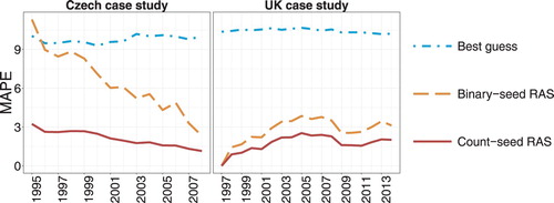
In both case studies, the reclassification method that most closely replicates the benchmark vectors is count-seed RAS. In the time periods in which the method is most inaccurate, its MAPE is in the region of 3%. As one would expect, the accuracy of RAS-based reclassification tends to gradually deteriorate as one moves to time periods further removed from the base year. Even so, the count-seed RAS method remains significantly more accurate than the best-guess approach throughout the time period of interest. This holds true not only in the Czech case study, in which the count-seed RAS contingency table estimate has already been found to be the most accurate of the lot, but also in the UK case, in which the best-guess approach actually outperforms the count-seed RAS method in contingency table estimation. In fact, the best-guess bridge matrix generally displays worse reclassification accuracy than not only count-seed RAS, but also binary-seed RAS.

While the results of Figure 1 provide a summary assessment of the overall degree of similarity between reclassified vectors produced by various methods and the benchmark reclassification, Figure 2 reports the results of comparisons conducted element by element. For selected years, we calculate the percentage difference between corresponding elements of the reclassified vectors and the appropriate benchmark vectors. The distribution of the percentage deviations is summarized in a boxplot.

FIGURE 2. Element-by-element percent deviation from the benchmark reclassification.

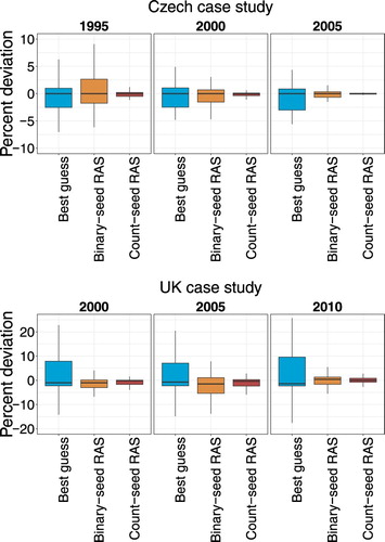
In the Czech case study, regardless of what conversion method is used, estimated gross output lies fairly close to the benchmark for the bulk of the 64 NACE Rev. 2 industries that make up the reclassified vector. In the reclassifications based on the binary-seed RAS or best-guess bridge matrix, however, it is not uncommon to observe industries for which estimated gross output is several percentage points off the value obtained from the true base-year bridge matrix. By contrast, the percent deviations associated with count-seed RAS re-classification are tightly clustered around zero. Over time, the behavior of the various reclassification approaches evolves consistently with what was already observed in Figure 1. The count-seed RAS bridge matrix reproduces the benchmark reclassification quite accurately throughout the period of interest. Binary-seed RAS reclassification, on the other hand, behaves well close to the base year, but becomes increasingly imprecise as time periods further removed from 2008 are considered. In the early years, its performance is comparable to that of the best-guess approach.

The UK results in Figure 2 are broadly in line with the analysis of Figure 1. Again, the approach that best approximates the benchmark vectors is count-seed RAS.

In our case study analysis, we have encountered several instances in which a comparatively accurate contingency table estimate turns out, somewhat counterintuitively, to produce a comparatively inaccurate reclassification. Most obviously, this occurs in the UK case, in which the best-guess contingency table estimate is the one that lies closest to the base-year table but performs worse than both binary-seed and count-seed RAS when it comes to recovering the benchmark reclassification. A similar reversal, however, is also observed in the Czech case study: in most of the years covered by the analysis, binary-seed RAS reclassification approximates the benchmark better than best-guess reclassification, in spite of the latter producing a more accurate contingency table estimate. The root of these results lies in the fact that RAS-based contingency table estimates do match the base-year table's marginal totals, whereas the best-guess bridge matrix does not. Because it is structurally inconsistent with those totals, the best-guess bridge matrix does not replicate the base-year benchmark and remains some way off throughout the period under analysis. Of the two RAS-based contingency table estimates, however, it is the one with the lowest dissimilarity from the base-year table that best approximates the benchmark reclassification.

5. Evidence from Monte Carlo simulations

5.1. Simulation framework

We further explore the data reclassification problem using Monte Carlo simulation methods. Each simulation is approached as follows. The analysis spans two time periods: a base year and a reclassification year. We start by randomly generating a base-year fundamental vector, as well as two suitably sized aggregation matrices that represent the source and the target classification. From these inputs, the base-year contingency table ${\mathbf{\text{C}}}^{\mathbf{\text{o}}}$ is computed as in Equation (5). As in the previous section, we first of all assess how closely count-seed RAS and other estimation approaches approximate the base-year contingency table. We then proceed to evaluate reclassification accuracy. To this end, it is assumed that each element of the fundamental vector evolves over time at its own specific growth rate. Thus, the reclassification-year value of a generic element of the fundamental vector is computed from its base year value as $x_i=\left(1+g_i\right)x_i^{\mathrm{o}}$, where $g_i$ represents a randomly selected rate of change. The reclassification-year source and the target vectors are obtained immediately by aggregation.

We reclassify the source vector using various alternative approaches and compare the results to the true target vector. This represents an important departure from the analysis of the previous section. In the case studies, because the true value of the target vector is inherently unobservable outside the base year, reclassification methods were assessed for their ability to replicate the benchmark reclassification produced using the base-year contingency table. By contrast, in a simulation study it becomes possible to evaluate all reclassification methods – including the benchmark reclassification itself – against the true target vector.

5.2. Parametric assumptions

We posit that the need for reclassification arises from a revision of the industry classification underlying the national accounts, and that the economic variable of interest is gross output. Accordingly, the same terminology is used as in Section 2, with the fundamental items referred to as products and aggregates as industries. Having narrowed down the problem, we are able to identify a range of realistic parameter values for our simulation study. Informed by a preliminary analysis of EU industrial production statistics at the 4-digit level of the Prodcom classification, the following assumptions are made. The base-year fundamental vector consists of 1000 independent draws from a lognormal distribution with parameters 5 and 1.5. This parametrization seems plausible in the context of a fairly large European economy. The product-specific growth rates are randomly selected on the basis of a normal distribution with mean ${\mu }_g=0.1$ and standard deviation ${\sigma }_g=0.15$. The source and the target classification are each assumed to consist of 100 industries. The source classification is generated by randomly assigning industries to products with uniform probability. The target classification is obtained by modifying the source classification: a pre-specified number of products, $k=250$, is randomly selected and re-allocated to a different industry aggregate. The probability that product $i$ is selected for reassignment is inversely proportional to $x_i^{\mathrm{o}}$. This is meant to reflect the empirical observation that classification revisions rarely modify the core constituent of the aggregates. A product selected for re-assignment is shifted to a new industry drawn at random with uniform probability.

We perform one thousand simulations. In each run, we attempt to recover the base-year table using the naive, the best-guess, the binary-seed and the count-seed RAS method. Using the U, WAD and STPE metrics, we assess the amount of estimation error associated with each of those approaches. We then examine each method’s reclassification performance in terms of MAPE and APE90. Reclassification schemes are evaluated not only against each other, but also in relation to the benchmark reclassification.

With regard to the best-guess approach, emulating the analyst's subjective judgment within an automated simulation process is challenging. We speculate that, in general, analysts can accurately assess how closely a certain pair of source and target industries is related. When the link is weak, however, the analyst might fail to recognize its existence. Based on this reasoning, we construct the best-guess conversion factors by knocking off the elements of the base-year bridge matrix that fall below a certain threshold. Thus, we create a truncated version of the base-year contingency table by replacing a given element $c_{ij}^{\mathrm{o}}$ of ${\mathbf{\text{C}}}^{\mathbf{\text{o}}}$ with zero whenever $b_{ij}^{\mathrm{o}}$ is less than a certain cutoff value. We then use the truncated matrix as the basis for computing the best-guess bridge matrix. We experiment with two cutoff values, 10% and 20%.

5.3. Simulation results

The distribution of key error measures over simulation runs is summarized for several reclassification methods in Table 4. The symbols M and SD respectively refer to the mean and the standard deviation of the simulated distributions. Across dissimilarity metrics, the best-guess approach systematically yields the most faithful representation of the base-year contingency table. This holds true even when the cutoff value used in the construction of the best-guess estimate is relatively high. When it comes to reclassification accuracy, however, RAS-based methods generally perform better than best-guess approaches. As shown in the rightmost columns of Table 4, the MAPE and APE90 distributions associated with RAS-based reclassification have comparatively lower values of both M and SD. Even though best-guess reclassification does occasionally display lower MAPE than binary-seed RAS (in 19 out of 1000 simulations), both are outperformed by count-seed RAS in each and every simulation run. These differences in reclassification performance between best-guess and RAS-based approaches can be visually appreciated from Figure C1 in Appendix C (online supplemental material), which represents the joint distribution of MAPE over simulation runs for selected pairs of methods. A similar analysis performed on the distribution of APE90 would lead to the same conclusions. Taken together, these results seem compatible with the findings of the case study analysis in Section 4.

TABLE 4. Summary statistics for the simulated distribution of key error measures

	Contingency table estimation						Reclassification
	U		WAD		STPE		MAPE		APE90
	M	SD	M	SD	M	SD	M	SD	M	SD
Naive	64	7.4	245	4.5	68	147.9	31.2	6.26	65.3	14.32
Best guess (20% threshold)	6	1.3	9	0.9	8	1.8	6.7	1.01	16.3	3.08
Best guess (10% threshold)	4	0.8	8	0.7	6	1.5	5.2	0.74	12.1	2.03
Binary-seed RAS	40	7.0	89	7.7	63	17.3	3.6	0.47	8.8	1.34
Count-seed RAS	14	2.1	30	2.3	22	6.0	1.9	0.25	4.4	0.76
Benchmark	0	0	0	0	0	0	1.0	0.19	2.5	0.57

Legend: M, mean; SD, standard deviation.

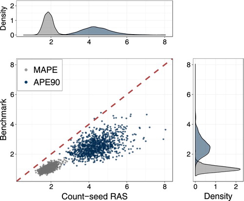
Being satisfied that in our simulation count-seed RAS reclassification is unambiguously superior to either the binary-seed RAS or the best-guess method, we turn to assessing its accuracy in relation to the benchmark reclassification. The joint and marginal distributions of MAPE and APE90 for count-seed RAS and benchmark reclassification are represented in Figure 3. Unsurprisingly, reclassification is more accurate if the bridge matrix is computed from ${\mathbf{\text{C}}}^{\mathbf{\text{o}}}$ itself rather than from the count-seed RAS estimate thereof. Nevertheless, the additional reclassification bias that results from lacking access to the true base-year conversion factors seems relatively small. The distribution of the MAPE for the benchmark reclassification is roughly centered around 1%. By contrast, averaging the MAPE associated with count-seed RAS over simulation runs yields a mean error of approximately 2%. The mean APE90 is 2.5% for the benchmark and 4.4% for count-seed RAS reclassification.

FIGURE 3. Reclassification accuracy: count-seed RAS versus benchmark reclassification.

5.4. Sensitivity analysis

While encouraging, the findings of Subsection 5.3 are obviously tied to the specific parametric assumptions used in the simulation. To assess how significantly modifying those assumptions would affect our results, we perform a sensitivity analysis with respect to the number of products selected for reclassification ($k$) and to the standard deviation (${\sigma }_g$) of the distribution from which the product-specific growth rates are sampled.

Intuitively, increases in $k$ and sigma ${\sigma }_g$ both make the reclassification problem more challenging. A larger value of $k$ indicates a deeper revision of the industry classification. The parameter ${\sigma }_g$, on the other hand, can be thought of as an expeditious way of modeling how far apart in time the reclassification and the base year are from each other. In the baseline simulations of Subsection 5.3, industry assignment is changed for one fourth of the economy's products and a fairly significant diversity of growth rates among products is already allowed for. The sensitivity analysis considers parameter values both above and below those baseline levels. Specifically, we report simulation results for $k\in \left\{100,250,500\right\}$ and ${\sigma }_g\in \left\{0.05,0.15,0.25\right\}$.

In addition, we examine the implications of assuming that the probability of a product being selected for re-assignment during classification revisions is inversely proportional to output. We thus run an alternative set of simulations in which that assumption is dropped and products are sampled for re-assignment independently with uniform probability. This also tends to increase the difficulty of the reclassification exercise, as it makes it more likely that the core constituents of any given industry are modified.

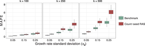
For each combination of parameter values, we run one thousand simulations and contrast the reclassification performance of the count-seed RAS method with that of the benchmark reclassification. The boxplots in Figure 4 show how the simulated distribution of MAPE changes as we vary $k$ and ${\sigma }_g$ while retaining the assumption of re-assignment probability inversely proportional to output. As expected, irrespective of what parametric assumptions are used in the simulations, the MAPE distribution is centered at lower values in the case of the benchmark reclassification than in the case of count-seed RAS reclassification. Instances of the count-seed RAS method attaining a lower MAPE than the benchmark reclassification in individual simulations exist but are negligibly rare. The accuracy of both approaches worsens with an increase in either $k$ or ${\sigma }_g$. As the reclassification problem becomes more difficult, the gap in accuracy between methods widens.

FIGURE 4. Simulated MAPE distribution under varying parametric assumptions.

A similar pattern can be seen in the top panel of Table 5, which reports the mean and standard deviation of the simulated distribution not only for MAPE but also for APE90. In addition, the bottom panel contemplates scenarios with uniform probability of re-assignment. From a comparison between the panels of Table 5, it is apparent that – once every product is given the same probability of moving to a new industry – error levels become noticeably higher for both the benchmark and the count-seed RAS reclassification. At the same time, however, the difference in reclassification accuracy between the two approaches seems to shrink. With $k=250$ and ${\sigma }_g=0.15$, for example, when the product reallocation mechanism is modified, the mean APE90 associated with the benchmark reclassification grows from 2.5% to 7.2%. While the accuracy of count-seed RAS reclassification also deteriorates, the difference in mean APE90 between the two methods drops from 1.9 to 0.8 percentage points.

TABLE 5. Simulated MAPE and APE90 distributions under varying assumptions.

		MAPE				APE90
		M		SD		M		SD
$k$	${\sigma }_g$	BM	RAS	BM	RAS	BM	RAS	BM	RAS
With probability of reassignment inversely proportional to output
100	0.05	0.1	0.2	0.04	0.04	0.3	0.5	0.10	0.10
100	0.15	0.4	0.5	0.11	0.12	1.0	1.3	0.31	0.35
100	0.25	0.7	0.9	0.19	0.21	1.7	2.1	0.52	0.60
250	0.05	0.3	0.6	0.06	0.08	0.8	1.5	0.18	0.24
250	0.15	1.0	1.9	0.19	0.25	2.5	4.4	0.57	0.76
250	0.25	1.7	3.1	0.31	0.45	4.2	7.4	0.91	1.28
500	0.05	0.7	1.2	0.09	0.12	1.7	2.7	0.27	0.34
500	0.15	2.1	3.6	0.27	0.38	5.0	8.0	0.82	1.05
500	0.25	3.6	6.2	0.46	0.66	8.4	13.4	1.35	1.77
With uniform probability of reassignment
100	0.05	0.5	0.6	0.10	0.09	1.5	1.5	0.31	0.31
100	0.15	1.7	1.7	0.30	0.30	4.4	4.6	0.99	1.01
100	0.25	2.8	2.9	0.50	0.51	7.5	7.6	1.62	1.62
250	0.05	1.0	1.2	0.11	0.13	2.4	2.7	0.35	0.39
250	0.15	3.0	3.4	0.36	0.40	7.2	8.0	1.05	1.15
250	0.25	5.1	5.8	0.63	0.71	12.1	13.3	1.84	2.05
500	0.05	1.4	1.7	0.13	0.16	3.0	3.5	0.34	0.41
500	0.15	4.1	5.0	0.42	0.52	8.9	10.6	1.09	1.27
500	0.25	7.0	8.5	0.73	0.92	15.0	17.9	1.93	2.32

Legend: M, mean; SD, standard deviation; BM, benchmark; RAS, count-seed RAS.

Overall, our sensitivity analysis suggests that, across a broad range of realistic parameter values, the cost in terms of reclassification accuracy of surrogating an unknown bridge matrix with the corresponding count-seed RAS estimate is generally modest. In the majority of scenarios, count-seed RAS reclassification results in error levels that would be tolerable in most empirical applications. Estimates of target industry output that are more than a handful of percentage points off the mark are only commonplace in fairly pathological scenarios (e.g. when half of the economy's products have their industry of assignment changed and product-specific growth rates are extremely diverse). In those cases, however, the benchmark reclassification also tends to be quite inaccurate.

6. Concluding remarks

How can one link two heavily aggregated datasets that are organized according to different statistical classifications? Although seldom discussed in the literature, this data management problem arises very often in applied work. Inside statistical institutes, data are typically converted between classifications using bridge matrices constructed from microdata. Such bridge matrices, however, are not generally accessible to independent researchers. This paper put forward a simple and flexible way of handling data reclassification in the very common case in which a bridge matrix grounded in microdata cannot be obtained.

The proposed approach is designed to take advantage of information that is readily available under most circumstances. We note that in applications there is typically a time period – or a geographical area that is comparable to the one of interest – for which the economic variable in question can be observed according to both the source and the target classification. Also, qualitative but detailed correspondences between elementary items can be easily retrieved from official sources for virtually any pair of statistical classifications. From this information, a bridge matrix linking the two classifications is constructed using bi-proportional scaling methods. We refer to our approach as count-seed RAS.

After illustrating the mechanics of the method through a simple numerical example, we assessed its performance in two case studies. Our findings suggest that the count-seed RAS approach is a cost-effective and quite accurate way of reverse engineering the official data reclassification carried out by a statistical institute. Notably, the count-seed RAS approach appears to perform significantly better in terms of reclassification accuracy than other expeditious methods commonly used by researchers to get around classification problems.

Count-seed RAS reclassification was further tested using Monte Carlo methods. Overall, the findings are consistent with what was observed in the case studies. Across a wide range of realistic scenarios, we observe that the reclassification error associated with count-seed RAS lies comfortably within the limits of what would be considered tolerable in empirical applications. In addition, our simulations suggest that replacing a bridge matrix based on microdata with an estimate constructed by count-seed RAS generally comes at a fairly modest cost in terms of additional reclassification error. In other words, the data reclassification obtained by count-seed RAS can be expected not to depart much from the one the statistical office would produce. In the most challenging scenarios, the count-seed RAS reclassification does turn out to be quite inaccurate. In the majority of those cases, however, the reclassification based on the microdata also displays significant levels of reclassification error.

Our study has focused primarily on situations in which the need for reclassification stems from a revision of the industry classification adopted by the national accounts. Also, in all the examples considered here, the data at the heart of the reclassification problem take the form of a vector of observations on a single variable. Nevertheless, we argue that the array of problems that can be handled by count-seed RAS is broader. For instance, one of the case studies demonstrated its use for the conversion of household consumption data from a classification by purpose to one by-product. A RAS-based approach could also be employed in the reclassification of supply-and-use or input–output tables. In a project recently concluded at the European Commission's Joint Research Centre, for example, the count-seed RAS approach was used to convert the intercountry input–output tables developed by the Organization for Economic Co-operation and Development between revisions 3 and 4 of the International Standard Industrial Classification.

In spite of our encouraging experience, it must not be forgotten that the count-seed RAS approach represents a sub-optimal solution to the data reclassification problem. Indeed, if the conversion factors used in the compilation of published statistics were accessible, researchers would be able to reclassify their data in a manner that is both more accurate and timelier. In this respect, we believe that statistical offices should be encouraged to systematically release bridge matrices (and, in a broader sense, similar intermediate products of their institutional activities) to the public.

Finally, we believe that the utility of the analytical framework underlying this study goes beyond justifying the use of a simple mechanical data reclassification procedure in the absence of reliable ready-made conversion factors. As exemplified by our simulation analysis, the proposed framework provides a lens through which to assess the empirical significance of reclassification error even in those cases in which a bridge matrix based on microdata is used in applied work. In a similar spirit, it could be used to shed light on questions pertaining to the spatial portability and intertemporal stability of bridge matrices such as those raised by Kronenberg (2011). We speculate that the mathematical and statistical properties of the proposed framework might be worthy of further exploration.

Acknowledgments

The authors would like to thank Petr Musil and his colleagues at the Czech statistical office for sharing data and information regarding their reclassification practices. Mattia Cai gratefully acknowledges the funding received in the early stages of this work from his previous employer, the Free University of Bolzano-Bozen, Italy. Responsibility for the information and views expressed in this article lies entirely with the authors.

Disclosure statement

No potential conflict of interest was reported by the authors.

Notes

1 In real-world applications, convergence may also be hindered by the fact the base-year source and target vectors used to balance the seed matrix come from different vintages and are thus not entirely consistent with each other (e.g. they do not add up to the same grand total).

References

- Cai, M. (2016) Greenhouse gas Emissions from Tourist Activities in South Tyrol: A Multiregional Input–Output Approach. Tourism Economics, 22, 1301–1314. doi: 10.1177/1354816616669008
- Capros, P., D. Van Regemorter, L. Paroussos, P. Karkatsoulis, C. Fragkiadakis, S. Tsani, I. Charalampidis, and T. Revesz (2013) GEM-E3 model documentation. JRC-IPTS Working Papers, JRC83177, Joint Research Centre.
- Drew, S. and M. Dunn (2011) Blue Book 2011: Reclassification of the U.K. Supply and Use Tables. Office for National Statistics. Available at: http://www.ons.gov.uk/ons/rel/input-output/input-output-supply-and-use-tables/reclassification-of-the-uk-supply-and-use-tables/reclassification-of-the-uk-supply-and-use-tables-pdf.pdf [Accessed on June 8, 2017].
- Eurostat (2008) Eurostat Manual of Supply, use and Input-Output Tables. Luxembourg, Eurostat.
- Idel, M. (2016) A review of matrix scaling and Sinkhorn's normal form for matrices and positive maps. arXiv:1609.06349.
- Jackson, R. and A. Murray (2004) Alternative Input-Output Matrix Updating Formulations. Economic Systems Research, 16, 135–148. doi: 10.1080/0953531042000219268
- Kratena, K., G. Streicher, S. Salotti, M. Sommer, and J. M. Valderas Jaramillo (2017) FIDELIO 2: Overview and theoretical foundations of the second version of the Fully Interregional Dynamic Econometric Long-term Input-Output model for the EU-27. JRC-IPTS Working Papers, JRC105900, Joint Research Centre.
- Kronenberg, T. (2011) On the Intertemporal Stability of Bridge Matrix Coefficients. Paper Prepared for the 19th Input-Output Conference, June 13–17, Alexandria, USA.
- Lahr, M.L. and L. De Mesnard (2004) Biproportional Techniques in Input-Output Analysis: Table Updating and Structural Analysis. Economic Systems Research, 16, 115–134. doi: 10.1080/0953531042000219259
- Lenzen, M., B. Gallego and R. Wood (2009) Matrix Balancing Under Conflicting Information. Economic Systems Research 21, 23–44. doi: 10.1080/09535310802688661
- Lenzen, M. and S. Lundie (2012) Constructing Enterprise Input-Output Tables-a Case Study of New Zealand Dairy Products. Journal of Economic Structures, 1, 6. doi: 10.1186/2193-2409-1-6
- Lenzen, M., M.C. Pinto de Moura, A. Geschke, K. Kanemoto, and D.D. Moran (2012) A Cycling Method for Constructing Input–Output Table Time Series From Incomplete Data. Economic Systems Research, 24, 413–432. doi: 10.1080/09535314.2012.724013
- Lomax, N. and P. Norman (2016) Estimating Population Attribute Values in a Table: “get me started in” Iterative Proportional Fitting. The Professional Geographer, 68, 451–461. doi: 10.1080/00330124.2015.1099449
- Miller, R.E. and P.D. Blair (2009) Input-output Analysis: Foundations and Extensions. Cambridge, Cambridge University Press.
- ONS (2017) CPA-COICOP converter for household consumption, 2013. United Kingdom Office for National Statistics. Available at: http://www.ons.gov.uk/economy/nationalaccounts/uksectoraccounts/adhocs/006611cpacoicopconverterforhouseholdconsumption2013 [Accessed on December 20, 2017].
- Perani, G. and V. Cirillo (2015) Matching industry classifications. A method for converting NACE Rev. 2 to NACE Rev. 1. Working Papers Series in Economics, Mathematics and Statistics, University of Urbino. Available at: http://www.econ.uniurb.it/RePEc/urb/wpaper/WP_15_02.pdf [Accessed on June 8, 2017].
- R Core Team (2016) R: A Language and Environment for Statistical Computing. Vienna, R Foundation for Statistical Computing.
- Rueda-Cantuche, J.M., A.F. Amores, and I. Remond-Tiedrez (2013) Evaluation of different approaches to homogenise supply-use and input-output tables with common product and industry classifications, Report to the European Commission's Joint Research Centre under the Contract Project: “European and Euro Area Time Series of Supply, Use and Input-Output Tables in NACE Rev.2, current and previous year prices (2000-2009)” [available upon request]
- Smith, P.A. and G.G. James (2017) Changing Industrial Classification to SIC (2007) at the U.K. Office for National Statistics. J Off Stat, 33, 223–247. doi: 10.1515/jos-2017-0012
- United Nations Statistical Commission (2009) System of National Accounts 2008. New York, United Nations.
- Yuskavage, R.E. (2007) Converting historical industry time series data from SIC to NAICS. U.S. Department of Commerce Bureau of Economic Analysism.