Projecting supply and use tables: new variants and fair comparisons

ABSTRACT

We have introduced in this paper new variants of two methods for projecting Supply and Use Tables that are based on a distance minimisation approach (SUT-RAS) and the Leontief model (SUT-EURO). We have also compared them under similar and comparable exogenous information, i.e.: with and without exogenous industry output, and with explicit consideration of taxes less subsidies on products. We have conducted an empirical assessment of all of these methods against a set of annual tables between 2000 and 2005 for Austria, Belgium, Spain and Italy. From the empirical assessment, we obtained three main conclusions: (a) the use of extra information (i.e. industry output) generally improves projected estimates in both methods; (b) whenever industry output is available, the SUT-RAS method should be used and otherwise the SUT-EURO should be used instead; and (c) the total industry output is best estimated by the SUT-EURO method when this is not available.

KEYWORDS:

• SUT-EURO
• SUT-RAS
• updating
• projection
• supply and use tables

1. Introduction

Several reasons may explain the large amount of non-survey methods developed over the past 50 years for the construction of input–output tables (IOTs) and one of the most relevant ones is timeliness. IOTs are usually constructed based on detailed surveys once every five years and supply and use tables (SUTs) tend to be published annually (e.g. in the European Union). Reducing the timeliness of publication of these tables is difficult due to the considerable economic, technical and human resources required to collect and elaborate the appropriate data. Moreover, the time gap between the year of publication and the year of reference of the supply, use and input–output tables (SUIOTs) usually worsens this delay.¹ As a result, official SUIOTs are often published too late to be useful for policy-oriented research, which leads to the substantiation of the use of non-survey methods.

Besides timeliness, there are other reasons leading to the use of non-survey methods such as: (a) the need to construct homogeneous and regular time series of inter-country SUIOTs, which includes the estimation and projection of missing national SUIOTs; (b) the need to revise past published SUIOTs in order to adapt them to a new system of national accounts or a new classification of products/activities; (c) the need to balance and treat confidential values. In some of these cases, most of the elements of the SUIOTs to be produced are known, including row and/or column totals; but, occasionally, some specific cells, and/or subset of cells, are missing due to their low reliability or simply because they have been removed for confidentiality reasons. In all these situations, the use of non-survey methods is fully justified; and (d) the need for ‘regionalisation’, the construction of regional or sub-national SUIOTs starting from an available national SUIOT and exogenous statistical information for the region constitutes another field where the application of non-survey methods is crucial. Not only territorial disaggregation, also temporal disaggregation of SUIOTs is a field where the use of non-survey methods is promising.

The literature about non-survey methods for the construction of IOTs is prolific and quite extensive; Jackson and Murray (2004) and Lahr and de Mesnard (2004) provide general reviews of the most representative non-survey methods for the construction of IOTs. Regarding ‘regionalisation’ of IOTs, Hewings (1969, 1977) and Mainar-Causapé et al. (2017) are good examples of both the pioneering and the most recent related references. In what concerns SUTs projections, most of the non-survey methods were originally developed having in mind IOTs projections; however, some can be also applied or adapted for the projection of SUTs, handling negative elements and avoiding negative solutions (Temurshoev et al., 2011). First examples of projecting SUTs can be found in Dalgaard and Gysting (2004), Timmer et al. (2005) and Beutel (2008). Other pioneer works for estimating commodity-by-industry tables in a regionalisation context are Jackson (1998), Lahr (2001) or Gallego and Lenzen (2009).

The next section makes a summary and provides the context for the discussion on non-survey methods provided by the literature for the construction of SUTs; particularly, the SUT-RAS (Temurshoev and Timmer, 2011) and the SUT-EURO methods (Beutel, 2008).

2. Joint estimation of SUTs

Non-survey methods for IOTs can be used for the construction of SUTs. However, practical difficulties arise, avoiding their straightforward application. Should we want to apply GRAS, for example, then the total sum of rows (product output) and columns (industry output) of the SUTs for the target year must be known in advance; however, the product output is almost always missing from the National Accounts data.

Yet, it is possible to construct SUTs with one-sided type methods such as the EUKLEMS method (Timmer et al., 2005), the Proportional Correction Method (Eurostat, 2008) and the Statistical Correction Method (Eurostat, 2008). However, these methods usually perform worse than other bi-proportional methods – such as the RAS family of methods – since they do not use all information available or they lead to arbitrary adjustments in some parts of the SUTs (Temurshoev et al., 2011 and Temurshoev and Timmer, 2011).

Nowadays, it is well proven that the GRAS method (Günlük–Senesen and Bates, 1988; Junius and Oosterhaven, 2003) generally performs better than the rest of the other methods (Huang et al., 2008; Temurshoev et al., 2011). Nonetheless, one of the requirements of the GRAS method is that totals by rows and columns must be known for the target year and, as mentioned before, this is a quite strong practical limitation for updating SUTs since product output is not usually part of the cluster of estimations provided by Statistical Offices in their Economic Accounts. Other methods, such as the EUKLEMS or the EURO method adapted for SUTs (Beutel, 2008) are alternatives for the projection of SUTs when product outputs are unknown. Furthermore, Temurshoev and Timmer (2011) developed the SUT-RAS method that does not require the availability of product outputs for the target year. The SUT-RAS method estimates SUTs in an integrated framework (cfr. Eurostat, 2008, p. 348) circumventing the problem of unavailability of product output totals. In short, SUT-RAS method is the generalisation of the GRAS method for estimating SUTs jointly in an integrated framework. This method was extensively used to construct the SUTs of the WIOD (www.wiod.org).

The SUT-RAS method is rather flexible since it can be applied to different price valuations such as basic and purchasers’ prices; or to domestic and imported uses, separately. Likewise, as other RAS-like indirect methods, the SUT-RAS method can be adapted for additional exogenous information, as long as it is not conflicting. The methods introduced in this article do not deal with issues such as managing potential conflicting information and reliability aspects of the exogenous information provided, nor other features such as non-unity coefficients in the constraints. Some alternatives that address these issues are the KRAS² method (Lenzen et al., 2009), the CFB algorithm of Dalgaard and Gysting (2004) and the most recent proposal of boundary tightening algorithm developed by Serpell (2018).

Following Temurshoev and Timmer (2011), the SUT-RAS method outperforms other SUT projection methods such as the adapted version of the EURO method for SUTs (henceforth denoted as SUT-EURO) or the EUKLEMS method.

Nevertheless, this statement should be revisited. The SUT-EURO and the SUT-RAS methods, as defined by these authors, do not actually use the same information, thus leading to unfair comparisons and misleading conclusions. The SUT-EURO method uses the minimum information available (see Table 1) for the target year compared to the other two alternatives, EUKLEMS or SUT-RAS. Hence, these last two methods will have correct values for total industry output and total intermediate inputs by industry while the SUT-EURO method will not. Therefore, it would have been surprising not to choose the SUT-RAS method as the best option, also considering that the EUKLEMS method is of the one-sided type.

TABLE 1. Information required for the target year by method.

Information for the target year	EUKLEMS	SUT-RAS	SUT-EURO
${\mathbf{x}}_t$ (total output by industry)	✓	✓	Not required
${\mathbf{u}}_t$ (total intermediate inputs by industry)	✓	Endogenous	Not required
${\mathbf{v}}_t$ (total gross value added by industry)	Endogenous	✓	✓
${\mathbf{y}}_t$ (overall final demand by user category)	✓	✓	✓
$m_t$ (overall total imports)	✓	✓	✓
Total values of trade margins, transport margins, VAT and taxes less subsidies on products	✓	Not required	Not required

Consequently, the asymmetry in the information used by the different methods leads to the conclusion that any statement on the good or poor performance of these methods cannot be attributed only to the methods themselves but also to the different information used as the starting point.

As shown in Table 1, the SUT-EURO method is the one that uses the minimum information of the target year. The SUT-RAS method requires an additional piece of information compared to the SUT-EURO method, i.e. the output by industry; and the EUKLEMS method requires additional information on trade and transport margins, taxes and subsidies on products.

In order to circumvent this caveat, we will introduce in this paper adapted versions of the SUT-RAS and SUT-EURO methods with identical benchmark information for both the reference and target years. By doing so, we can therefore guarantee fairer conclusions on the comparative performance of the two methods.

On top of this asymmetric information problem existing in past assessments of updating methods (e.g. Temurshoev and Timmer, 2011), none of the existing methods in the literature reflect explicitly³ and consistently the taxes less subsidies on products, as in National Accounts. Therefore, we will also introduce in this paper adapted versions of the SUT-RAS and SUT-EURO methods that explicitly use taxes less subsidies on products (TLS) as an integrated part of the updating process.

Estimating integrated SUT frameworks with the new versions of the SUT-EURO and SUT-RAS methods proposed in this paper, using the same benchmark information, and assessing their performance is a valuable exercise. From a theoretical point view, the development of these new methods will provide practitioners with new tools when dealing with the projection of SUTs with restricted or additional information. For instance, if industry output is missing, then the only choice would be the SUT-EURO method; that is why we have developed an adapted version of the SUT-RAS method that does not use industry output as exogenous information. On the contrary, if industry output were available, then the use of the SUT-EURO method would leave this important extra piece of additional information unused; that is why we have developed an adapted version of the SUT-EURO method that uses industry output as exogenous information. Otherwise, the SUT-RAS method would be the only choice for making projections under such circumstances.

The lack of an explicit treatment of TLS may occasionally lead to some ambiguities in the practical application of the SUT-RAS and SUT-EURO methods as defined by Beutel (2008) and Temurshoev and Timmer (2011). TLS are usually available in National Accounts and should not therefore constitute a barrier for the practical application of the methods introduced here. In fact, this piece of information ensures the consistency of the equations of the new projection methods in terms of National Accounts.

Hence, as shown in Table 2, we consider two scenarios according to the available information. In both scenarios, the reference year information is a complete set of SUTs of the base year (not shown in Table 2). The difference between both scenarios is the output by industry at basic prices.

TABLE 2. Required benchmark information scenarios for the target year.

Information for the target year	Scenario 1 (restricted)	Scenario 2 (unrestricted)
${\mathbf{x}}_{b,t}$ (total industry output, at basic prices)	Not available	✓
${\mathbf{v}}_{b,t}$ (total gross value added by industry, at basic prices)	✓	✓
${\mathbf{y}}_{p,t}$ (overall total final demand by user, category at purchasers’ prices)	✓	✓
$m_t$ (overall total imports, CIF values)	✓	✓
$tl{s}_t$ (overall total of taxes less subsidies on products)	✓	✓

A comparative performance of all these new methods has been carried out to see which one performs better and under which circumstances in terms of the available information. We have used a set of official annual SUTs for the years between 2000 and 2005 for Austria, Belgium, Italy and Spain. The results are described under two different restricted (industry output missing) and unrestricted scenarios (industry output available). This allows us to draw conclusions on the best method to be used depending on the available information.

The choice of the period 2000–2005 is made on the basis of three reasons: (a) macroeconomic stability of the period; (b) SUTs are compiled under a common European System of Accounts (ESA-95); and (c) SUTs are compiled under a common classification of products and activities (NACE Rev. 1.1).

3. The projection methods for SUTs

Table 3 shows the characterisation of the existing and new adapted versions of the SUT-EURO and SUT-RAS methods provided by this article. However, we have decided to focus our attention only on the novel contributions. For a full description of the original SUT-EURO and SUT-RAS methods, the references are Beutel (2008) and Temurshoev and Timmer (2011), respectively. Small numerical examples implementing such methods can be found in United Nations (2018 pp. 496–505).

TABLE 3. Characterisation of existing and adapted non-survey methods.

Method	Dom/Imp	TLS explicit	Industry output
SUT-EURO	Yes	No	Endogenous
SUT-RAS	Yes	No	Exogenous
endo-SUT-EURO	Yes	Yes	Endogenous
endo-SUT-RAS
exo-SUT-EURO	Yes	Yes	Exogenous
exo-SUT-RAS

In this section, we therefore describe the new methods for updating SUTs.⁴

The new methods treat TLS explicitly and separately, unlike the original SUT-EURO and SUT-RAS methods. These new methods also include a split for domestic and imported uses.⁵ For abbreviation purposes, we will denominate the new methods using the suffixes endo and exo. The use of the suffix endo indicates that industry output is not available and has to be estimated endogenously by the corresponding methods; the suffix exo indicates exactly the opposite. And, last but not least, the SUT-EURO methods admit two other variants depending on the use of the arithmetic or the geometric means in the construction of the updated Use Tables, i.e. endo-SUT-EURO-A, endo-SUT-EURO-G, exo-SUT-EURO-A and exo-SUT-EURO-G. More detailed derivation of the methods developed here are excluded here for the ease of readability but are provided in the online appendixes of this article along with numerical examples and scripts for implementation.

To begin with, let us assume that the original base year SUTs consist of the following components for all the methods:

• - Let ${\mathbf{U}}_{b,0}^d$ and ${\mathbf{U}}_{b,0}^m$ be the domestic and imported intermediate uses at basic prices, with dimension commodity by industry $\left(p\times r\right)$ .

• - Let ${\mathbf{Y}}_{b,0}^d$ and ${\mathbf{Y}}_{b,0}^m$ be the domestic and imported final demand matrices, with dimension commodity by final use category $\left(p\times f\right)$ .

• - Let ${\mathbf{V}}_{b,0}$ be the Make matrix $\left(r\times p\right)$ or the transposed Supply matrix.

• - Let ${\mathbf{v}}_0$ be the vector of gross value added by industry, with dimension $\left(r\times 1\right)$ .

• - Let $\mathbf{t}\mathbf{l}{\mathbf{s}}_0$ be the vector of taxes less subsidies on products, with dimension $\left(r+f\right)\times 1$ . In turn, this vector is split into two subvectors, one for intermediate uses and another one for final uses. $\mathbf{t}\mathbf{l}{\mathbf{s}}_0=\left(\begin{array}{c}{\mathbf{t}\mathbf{l}\mathbf{s}}_0^{ID}\\ {\mathbf{t}\mathbf{l}\mathbf{s}}_0^{FD}\end{array}\right)$

3.1 The SUT-EURO method with an explicit treatment of TLS

The single new feature of the endo-SUT-EURO method compared to the original SUT-EURO method (Beutel, 2008 and Temurshoev and Timmer, 2011) is the explicit treatment of TLS in the updating process.

This is done by allowing one extra row in the Use Table to include TLS. That is, instead of the initial use matrix $\left[\begin{array}{cc}{\mathbf{U}}_{b,0}^d& {\mathbf{Y}}_{b,0}^d\\ {\mathbf{U}}_{b,0}^m& {\mathbf{Y}}_{b,0}^m\end{array}\right]$ , the new Use Table is ${\overline{\mathbf{U}}}_0=\left[\begin{array}{cc}{\mathbf{U}}_{b,0}^d& {\mathbf{Y}}_{b,0}^d\\ {\mathbf{U}}_{b,0}^m& {\mathbf{Y}}_{b,0}^m\\ \mathbf{t}\mathbf{l}\mathbf{s}{{}_0^{ID}}^{\mathrm{\prime }}& \mathbf{t}\mathbf{l}\mathbf{s}{{}_0^{FD}}^{\mathrm{\prime }}\end{array}\right]$.

This use matrix is updated column-wise with a matrix of factors, $\widehat{{\mathbf{w}}_c}=\widehat{\left[\begin{array}{c}{\mathit{\delta }}^{\mathbf{v}}\\ {\mathit{\delta }}^{\mathbf{y}}\end{array}\right]}$ and by rows with another matrix of factors, $\widehat{{\mathbf{w}}_r}=\widehat{\left[\begin{array}{c}{\mathit{\delta }}^{\mathbf{v}}\\ {\mathit{\delta }}^{\mathbf{v}}\\ {\delta }^{tls}\end{array}\right]}$ where ${\mathit{\delta }}^{\mathbf{v}}$ stands for the vector of variation rates between the target year and the base year of the gross value added (GVA) by industry, ${\mathit{\delta }}^{\mathbf{y}}$ the vector of variation rates for final demand totals by user category, and ${\delta }^{tls}$ the variation rate of taxes less subsidies on products for the whole economy. These vectors are calculated from the available information, as reported in Table 1.

Next, the subsequent steps of the endo-SUT-EURO method fully coincide with the original SUT-EURO method, only the difference being a new correcting factor (i.e. tls) in the iterative procedure.

3.2 The SUT-EURO method with an explicit treatment of TLS and output by industry exogenously available

This new method of projection is basically an extension of the endo-SUT-EURO method but with industry output available. This variant of the SUT-EURO method has been created trying to maintain the essentials of the original SUT-EURO method.

Given that industry output is available this allows for the estimation of variation rates of intermediate consumption by industry ${\mathit{\delta }}^{IC}$ (at purchasers’ prices) and the estimation of variation rates of outputs by commodity ${\mathit{\delta }}^{\mathbf{q}}$ that replace the use of the variation rates of GVA in the estimation process. Since there is no convincing reason as to why GVA and output should grow at the same rate; for this reason, we will use the newly derived growth rates of commodity outputs and the growth rates of intermediate consumption instead. With the globalisation of economic activities, intermediate inputs have tended to grow more rapidly than GVA during the last decade (cfr. Beutel, 2008, p. 5).

Once these two new variation rates are incorporated, the rest of the projection algorithmic is similar to the original SUT-EURO method. The updating process elaborates all the elements in the Use framework in an iterative way till convergence is achieved. That is, all the variation rates coming from the updated projects must match the official ones coming from the exogenous information. Finally, once convergence is achieved, calculation of ${\mathbf{V}}_t$ is done⁶ assuming that shares of total commodity outputs across industries remain unchanged (Beutel, 2008, p. 9). A final remark, it is important to note that having industry output available makes no longer necessary the use of Model D (Eurostat, 2008 – or the so-called fixed product sales structure assumption⁷) in order to derive consistent SUTs. This is internally assured in the iterative process because of the exogenous industry output and the consistently calculated product output by means of constant market shares.

To sum up, we have developed two new extensions of the original SUT-EURO method (Beutel, 2008): endo-SUT-EURO and exo-SUT-EURO.

3.3 The SUT-RAS method with an explicit treatment of TLS and output by industry exogenously available

We start with this extension of the SUT-RAS method since it only differs from the original in the inclusion of the TLS. Tables 4 and 5 depict the integrated supply-use framework in the base year and the target year with the available information in each moment, along with a description of the two variants of the SUT-RAS methods.

TABLE 4. Integrated supply-use framework for the base year^a and accounting identities.

	Domestic products (p^d)	Imported products (p^m)	Industries (r)	Final demand (f)	Total
Domestic products (p^d)			${\mathbf{U}}_{b,0}^d$	${\mathbf{Y}}_{b,0}^d$	${\mathbf{U}}_{b,0}^d\cdot \mathit{\iota }+{\mathbf{Y}}_{b,0}^d\cdot \mathit{\iota }={\mathbf{q}}_{b,0}^d$
Imported products (p^m)			${\mathbf{U}}_{b,0}^m$	${\mathbf{Y}}_{b,0}^m$	${\mathbf{U}}_{b,0}^m\cdot \mathit{\iota }+{\mathbf{Y}}_{b,0}^m\cdot \mathit{\iota }={\mathbf{m}}_0$
TLS			$\mathbf{t}\mathbf{l}\mathbf{s}{}_0^{I{D}^{\mathrm{\prime }}}$	$\mathbf{t}\mathbf{l}\mathbf{s}{}_0^{F{D}^{\mathrm{\prime }}}$	$\mathbf{t}\mathbf{l}\mathbf{s}{}_0^{I{D}^{\mathrm{\prime }}}\cdot \mathit{\iota }+\mathbf{t}\mathbf{l}\mathbf{s}{}_0^{F{D}^{\mathrm{\prime }}}\cdot \mathit{\iota }=tl{s}_0$
Industries (r)	${\mathbf{V}}_{b,0}$				${\mathbf{V}}_{b,0}\cdot \mathit{\iota }={\mathbf{x}}_{b,0}$
Imports (m)		${\mathbf{m}}_0^{\mathrm{\prime }}$			${\mathbf{m}}_0^{\mathrm{\prime }}\cdot \mathit{\iota }=m_0$
Total	${\mathit{\iota }}^{\mathrm{\prime }}\cdot {\mathbf{V}}_{b,0}=\mathbf{q}{}_{b,0}^{d^{\mathrm{\prime }}}$	${\mathbf{m}}_0^{\mathrm{\prime }}$	${\mathbf{x}}_{b,0}^{\mathrm{\prime }}-{{\mathbf{v}}_{b,0}}^{\mathrm{\prime }}$	${\mathbf{y}}_{p,0}^{\mathrm{\prime }}$

^a All the elements in this table are known.

Similarly to the original SUT-RAS method (Temurshoev and Timmer, 2011), let $\mathbf{A}$ be our integrated supply-use framework for the base year, which is completely known⁸: (1) $\mathbf{A}=\left(\begin{array}{cc}{\mathbf{O}}_{{}_{\left(p^d+p^m+1\right)\times \left(p^d+p^m\right)}}& {\overline{\mathbf{U}}}_0\\ {\overline{\mathbf{V}}}_0& {\mathbf{O}}_{\left(r+m\right)\times \left(r+f\right)}\end{array}\right)\in {\mathcal{M}}_{\left(p^d+p^m+r+2\right)\times \left(p^d+p^m+r+f\right)}\left(1\right)$(1) where

• ${\overline{\mathbf{V}}}_0\in {\mathcal{M}}_{(r+m)\times \left(p^d+p^m\right)}=\left(\begin{array}{cc}{\mathbf{V}}_{b,0}& {\mathbf{O}}_{r\times p^m}\\ {\mathbf{0}}_{m\times p^d}& {{\mathbf{m}}_0}^{\mathrm{\prime }}\end{array}\right)$ , elements of the supply side for the base year (Table 5)

• ${\overline{\mathbf{U}}}_0\in {\mathcal{M}}_{\left(p^d+p^m+1\right)\times (r+f)}=\left(\begin{array}{cc}{\mathbf{U}}_{b,0}^d& {\mathbf{Y}}_{b,0}^d\\ {\mathbf{U}}_{b,0}^m& {\mathbf{Y}}_{b,0}^m\\ \mathbf{t}\mathbf{l}\mathbf{s}{}_0^{D{I}^{\mathrm{\prime }}}& \mathbf{t}\mathbf{l}\mathbf{s}{}_0^{D{F}^{\mathrm{\prime }}}\end{array}\right)$ , the extended Use matrix for the base year.

TABLE 5. Integrated supply-use framework for the target year^(*).

	Domestic products (p^d)	Imported products (p^m)	Industries (r)	Final demand (f)	Total
Domestic products (p^d)			${\mathbf{U}}_{b,t}^d$	${\mathbf{Y}}_{b,t}^d$	${\mathbf{U}}_{b,t}^d\cdot \mathit{\iota }+{\mathbf{Y}}_{b,t}^d\cdot \mathit{\iota }$
Imported products (p^m)			${\mathbf{U}}_{b,t}^m$	${\mathbf{Y}}_{b,t}^m$	${\mathbf{U}}_{b,t}^m\cdot \mathit{\iota }+{\mathbf{Y}}_{b,t}^m\cdot \mathit{\iota }$
TLS			$\mathbf{t}\mathbf{l}\mathbf{s}{}_t^{I{D}^{\mathrm{\prime }}}$	$\mathbf{t}\mathbf{l}\mathbf{s}{}_t^{F{D}^{\mathrm{\prime }}}$	$tl{s}_t$ ^(*)
Industries (r)	${\mathbf{V}}_{b,t}$				${\mathbf{x}}_{b,t}$ ^(*)
Imports (m)		${{\mathbf{m}}_t}^{\mathrm{\prime }}$			$m_t$ ^(*)
Total	${\mathit{\iota }}^{\mathrm{\prime }}\cdot {\mathbf{V}}_{b,t}$	${{\mathbf{m}}_t}^{\mathrm{\prime }}$	$\left({{\mathbf{x}}_{b,t}}^{\mathrm{\prime }}-{{\mathbf{v}}_{b,t}}^{\mathrm{\prime }}\right)$ ^(*)	${{\mathbf{y}}_{p,t}}^{\mathrm{\prime }}$ ^(*)

Only the elements with superscript ^(*) are known. The rest have to be estimated and unknown totals calculated by aggregation.

In an analogous way, let $\mathbf{X}$ stand for the supply-use integrated framework for the target year $t$ (2) $\mathbf{X}=\left(\begin{array}{cc}{\mathbf{O}}_{{}_{\left(p^d+p^m+1\right)\times \left(p^d+p^m\right)}}& {\overline{\mathbf{U}}}_t\\ {\overline{\mathbf{V}}}_t& {\mathbf{O}}_{\left(r+m\right)\times \left(r+f\right)}\end{array}\right)\in {\mathcal{M}}_{\left(p^d+p^m+r+2\right)\times \left(p^d+p^m+r+f\right)}\left(2\right)$(2) Starting from $\mathbf{A}$ , we must derive $\mathbf{X}$ in a consistent way using the exogenous additional information for the target year. The exogenous additional information and certain accounting equilibria coming from the integrated supply-use framework can be formulated as follows in the next block of equations:

Dom. production supply-use balance: $\left({\mathbf{U}}_{b,t}^d\cdot \mathit{\iota }+{\mathbf{Y}}_{b,t}^d\cdot \mathit{\iota }\right)-{{\mathbf{V}}_{b,t}}^{\mathrm{\prime }}\cdot \mathit{\iota }=\mathbf{0}$ (3)

Imports supply-use balance: $\left({\mathbf{U}}_{b,t}^m\cdot \mathit{\iota }+{\mathbf{Y}}_{b,t}^m\cdot \mathit{\iota }\right)={\mathbf{m}}_t$ (4)

Industry output preservation: ${\mathbf{V}}_{b,t}\cdot \mathit{\iota }={\mathbf{x}}_{b,t}$ (5)

Imports preservation: ${{\mathbf{m}}_t}^{\mathrm{\prime }}\cdot \mathit{\iota }=m_t$ (6)

Int. cons. preservation: $\mathbf{U}{}_{b,t}^d{}^{\mathrm{\prime }}\cdot \mathit{\iota }+\mathbf{U}{}_{b,t}^m{}^{\mathrm{\prime }}\cdot \mathit{\iota }+{\mathbf{t}\mathbf{l}\mathbf{s}}_t^{ID}={\mathbf{x}}_{b,t}-{\mathbf{v}}_t=\mathbf{I}{\mathbf{C}}_{p,t}$ (7)

Final demand preservation: $\mathbf{Y}{}_{b,t}^d{}^{\mathrm{\prime }}\cdot \mathit{\iota }+\mathbf{Y}{}_{b,t}^m{}^{\mathrm{\prime }}\cdot \mathit{\iota }+{\mathbf{t}\mathbf{l}\mathbf{s}}_t^{FD}={\mathbf{y}}_{p,t}$ (8)

TLS preservation: $\mathbf{t}\mathbf{l}\mathbf{s}{}_t^{ID}{}^{\mathrm{\prime }}\cdot \mathit{\iota }+\mathbf{t}\mathbf{l}\mathbf{s}{}_t^{FD}{}^{\mathrm{\prime }}\cdot \mathit{\iota }=tl{s}_t$ (9)

A crucial aspect to be noted is that since industry output and GVA are exogenous information for this method, we can use them to obtain the intermediate consumption at purchasers’ prices (as in the exo-SUT-EURO). This helps us to set up constraint (7).

The rest is setting up this optimisation problem with an objective function based on Huang et al. (2008) that operationalises transformation that must undertake the elements in A to become the updated elements of X, satisfying the above set of constraints.

3.4 The SUT-RAS method with an explicit treatment of TLS and output by industry derived endogenously

In this method, we return to the scenario where the industry outputs are not available for the target year. This leads to a rearrangement of our optimisation problem bearing in mind this fact. Since ${\mathbf{x}}_{b,t}$ is no longer exogenous, we must rely on the equilibrium features of the system to derive this information.

In order to circumvent this problem and pose our optimisation problem, Table 6 shows a revised integrated supply-use framework where industry output (${\mathbf{x}}_{b,t}$ ) is missing and has to be derived fully endogenously along with the rest of unknown elements in the framework. All the constraints in the optimisation problem have to be also revised and expressed only with the information available shown in Table 6.

TABLE 6. Integrated supply-use framework for the target year t ^(*).

	Domestic products (p^d)	Imported products (p^m)	Industries (r)	Final demand (f)	Total
Domestic products (p^d)			${\mathbf{U}}_{b,t}^d$	${\mathbf{Y}}_{b,t}^d$	${\mathbf{U}}_{b,t}^d\cdot \mathit{\iota }+{\mathbf{Y}}_{b,t}^d\cdot \mathit{\iota }$
Imported products (p^m)			${\mathbf{U}}_{b,t}^m$	${\mathbf{Y}}_{b,t}^m$	${\mathbf{U}}_{b,t}^m\cdot \mathit{\iota }+{\mathbf{Y}}_{b,t}^m\cdot \mathit{\iota }$
TLS			$\mathbf{t}\mathbf{l}\mathbf{s}{}_t^{I{D}^{\mathrm{\prime }}}$	$\mathbf{t}\mathbf{l}\mathbf{s}{}_t^{F{D}^{\mathrm{\prime }}}$	$tl{s}_t$ ^(*)
Industries (r)	${\mathbf{V}}_{b,t}$				${\mathbf{V}}_{b,t}\cdot \mathit{\iota }$
Imports (m)		${{\mathbf{m}}_t}^{\mathrm{\prime }}$			$m_t$ ^(*)
Total	${\mathit{\iota }}^{\mathrm{\prime }}\cdot {\mathbf{V}}_{b,t}$	${{\mathbf{m}}_t}^{\mathrm{\prime }}$	$({\mathbf{V}}_{b,t}\cdot \mathit{\iota }{)}^{\mathrm{\prime }}-{{\mathbf{v}}_{b,t}}^{\mathrm{\prime }}$ ^(*)	${{\mathbf{y}}_{p,t}}^{\mathrm{\prime }}$ ^(*)

Only the elements with superscript ^(*) are known. The rest have to be estimated and unknown totals calculated by aggregation.

Again, let $\mathbf{A}$ be our integrated supply-use framework for the base year, which is completely known, and let $\mathbf{X}$ stand for the supply–use integrated framework for the target year $t$ in the same way as in (1) and (2). The current exogenous additional information and accounting equilibria coming from the revised integrated supply-use framework (Table 6) can be formulated as follows:

Dom. production supply-use balance: $\left({\mathbf{U}}_{b,t}^d\cdot \mathit{\iota }+{\mathbf{Y}}_{b,t}^d\cdot \mathit{\iota }\right)-{{\mathbf{V}}_{b,t}}^{\mathrm{\prime }}\cdot \mathit{\iota }=\mathbf{0}$ (10)

Imports supply-use balance: $\left({\mathbf{U}}_{b,t}^m\cdot \mathit{\iota }+{\mathbf{Y}}_{b,t}^m\cdot \mathit{\iota }\right)={\mathbf{m}}_t$ (10)

Imports preservation: ${{\mathbf{m}}_t}^{\mathrm{\prime }}\cdot \mathit{\iota }=m_t$ (11)

Intermediate consumption balance: $\mathbf{U}{}_{b,t}^d{}^{\mathrm{\prime }}\cdot \mathit{\iota }+\mathbf{U}{}_{b,t}^m{}^{\mathrm{\prime }}\cdot \mathit{\iota }+{\mathbf{t}\mathbf{l}\mathbf{s}}_t^{ID}={\mathbf{V}}_{b,t}\cdot \mathit{\iota }-{\mathbf{v}}_{b,t}$ (12)

Final demand preservation: $\mathbf{Y}{}_{b,t}^d{}^{\mathrm{\prime }}\cdot \mathit{\iota }+\mathbf{Y}{}_{b,t}^m{}^{\mathrm{\prime }}\cdot \mathit{\iota }+{\mathbf{t}\mathbf{l}\mathbf{s}}_t^{FD}={\mathbf{y}}_{p,t}$ (13)

TLS preservation: $\mathbf{t}\mathbf{l}\mathbf{s}{}_t^{ID}{}^{\mathrm{\prime }}\cdot \mathit{\iota }+\mathbf{t}\mathbf{l}\mathbf{s}{}_t^{FD}{}^{\mathrm{\prime }}\cdot \mathit{\iota }=tl{s}_t$ (14)

With regard to comparisons, the set of restrictions in the exo-SUT-RAS (Equations (3) to (9)) compared to the set of restrictions in the endo-SUT-RAS (Equations (10) to (15)), we see that Equation (5) (Industry supply-use balance) is missing since ${\mathbf{x}}_{b,t}$ is no longer available and none of its elements are known. Even so, we use this balance in order to modify the rest of equations where ${\mathbf{x}}_{b,t}$ was necessary. With this link, the endo-SUT-RAS method does not lose its bivariate feature, and every element of matrix X will be obtained from column and row scaling factors. In this case, the number of vectors of factors in the solution will be reduced by one according to the reduction in the number of restrictions. The optimisation problem is set up and solved in an analogous way to the exo-SUT-RAS method.

4. Empirical assessment

The methods introduced in the previous section are applied to a set of benchmark SUTs of Austria, Belgium, Italy and Spain for the years ranging from 2000 to 2005. The data are disaggregated into 60 industries and 60 products (A60 classification) and 3 final use categories (consumption, gross capital formation and exports).

We have carried out, for each method (endo-SUT-EURO-A, endo-SUT-EURO-G, exo-SUT-EURO-A and exo-SUT-EURO-G, endo-SUT-RAS and exo-SUT-RAS), 5 one-year projections starting from 2000 up to 2005 (i.e. 2000–2001, 2001–2002, 2002–2003, 2003–2004, 2004–2005) and 1 five-year projection from 2000 to 2005. As described in previous sections, we used industry output as exogenous information in the exo-SUT-RAS and exo-SUT-EURO methods; while in the endo-SUT-RAS and endo-SUT-EURO methods industry output is estimated endogenously. In all cases, we use gross value added by industry at basic prices, final demand at purchasers’ prices by final use category, total imports (CIF) and total taxes less subsidies on products. The results of every projection have been compared to the official benchmark SUTs of the projected year. Eventually, we have selected a set of six measures of goodness of fit from the existing literature⁹ and tested the different methods in order to draw general conclusions independently of the time horizon of the projections and the country of reference.

4.1 Measures of goodness of fit

We have used the following criteria to assess the relative performance of every method:

1. Weighted Absolute Percentage Error (WAPE – Temurshoev et al, 2011) $WAPE=\sum _{i=1}^m\sum _{j=1}^n\left(\frac{|x_{ij}|}{\sum _{i=1}^m\sum _{j=1}^n|x_{ij}|}\right)\left|\frac{x_{ij}-\widetilde{x_{ij}}}{x_{ij}}\right|$

where $x_{ij}$ is the value of the element $\left(i,j\right)$ in the official benchmark SUTs of the projected year and $\widetilde{x_{ij}}$ is the corresponding estimated projection. WAPE averages relative errors with respect to the target value according to their size in absolute terms.

1. Mean Absolute Scaled Error (MASE – Hyndman and Koehler, 2006) $MASE=\sum _{i=1}^m\sum _{j=1}^n\left|\frac{m\cdot n}{\sum _{i=1}^m\sum _{j=1}^n|x_{ij}-\overline{x}|}\right||x_{ij}-\widetilde{x_{ij}}|$

This measure was first introduced in the field of time series analysis (Hyndman and Koehler, 2006) and has been adapted here for assessing the goodness of fit of the various projections. In our case, the MASE does not weight errors but scales them. That is, for each element (i,j), the absolute value of the errors are divided over the average of the absolute deviations of the target values with respect to their mean across all the elements of the table. This distinctive feature of the MASE indicator is that it can be calculated even if $x_{ij}=0$ , which is not the case for the WAPE indicator.

1. Weighted Absolute Scaled Error (WASE). $WASE=\sum _{i=1}^m\sum _{j=1}^n\left(\frac{|x_{ij}|}{\sum _{i=1}^m\sum _{j=1}^n|x_{ij}|}\right)\left|\frac{|x_{ij}-\widetilde{x_{ij}}|}{\sum _{i=1}^m\sum _{j=1}^n|x_{ij}-\overline{x}|/m\cdot n}\right|$

This is a generalisation of the MASE indicator (Hyndman and Koehler, 2006) where every scaled error (in absolute terms) is weighted by the size of the target coefficients in order to calculate an average of scaled errors.

The WAPE, MASE and WASE indicators have zero as a minimum and are not affected by changes in the scale of measure or by a shift in data or by the size of the coefficients in the table. However, none of them has a maximum threshold, which makes the comparisons across indicators more difficult. With this in mind, we have also considered the three more different indicators of goodness of fit:

1. Normalised Symmetric Weighted Average Proportional Error ($\rho -SWAPE$ – Arto et al, 2014)

This is a weighted version of the so-called Symmetric Absolute Mean Percentage Error statistic described in Hyndman and Koehler (2006, p. 683) $SWAPE=200\cdot \sum _{i=1}^m\sum _{j=1}^n\left(\frac{|x_{ij}|}{\sum _{i=1}^m\sum _{j=1}^n|x_{ij}|}\right)\left|\frac{x_{ij}-\widetilde{x_{ij}}}{x_{ij}+\widetilde{x_{ij}}}\right|$ The SWAPE indicator is bounded between 0 and 200. Hence, by normalising, we obtain: $\rho -SWAPE=100\cdot \left(1-\frac{SWAPE}{200}\right)$ where 1 stands for the best fit and 0 for the worst fit.

1. Normalised psi Statistic ($\rho -PSI$ – Kullback and Leibler, 1951 and Kullback, 1959)

This is a normalisation of a modified version of the psi statistic of Kullback ready to use for matrices with arbitrary elements that can be positive, negative or zero. Sign shifts between the elements of the estimated table and the benchmark table are allowed.

Let the modified version of the psi statistic of Kullback (henceforth denoted as $\rho -PSI$) be: $\overline{\overline{\psi \left(X,\tilde{X}\right)}}=\sum _{i=1}^m\sum _{j=i}^n|x_{ij}|\ln \frac{|x_{ij}|}{\left(\frac{|x_{ij}|+|\widetilde{x_{ij}}|}{2}\right)}+\sum _{i=1}^m\sum _{j=i}^n|\widetilde{x_{ij}}|\ln \frac{|\widetilde{x_{ij}}|}{\left(\frac{|x_{ij}|+|\widetilde{x_{ij}}|}{2}\right)}$ This $\rho -PSI$ is bounded as follows: $0\le \overline{\overline{\psi \left(X,\tilde{X}\right)}}\le \ln 2\cdot \sum _{i=1}^m\sum _{j=1}^n\left(|x_{ij}|+|\widetilde{x_{ij}}|\right)$

hence: $\rho -PSI=100\cdot \frac{\overline{\overline{\psi \left(X,\tilde{X}\right)}}}{\ln 2\cdot \sum _{i=1}^m\sum _{j=1}^n\left(|x_{ij}|+|\widetilde{x_{ij}}|\right)}$ so $\rho -PSI$ is bounded between 0 and 1 (0 being the worst fit and 1 the best fit).

1. Similarity Index (Szyrmer, 1989)

The similarity index is a linear transformation of the correlation coefficient between the target values and the estimated values (inspired on the dissimilarity index of. Szyrmer (1989)) $IS=50\cdot \left(1+r_{X,\tilde{X}}\right)$ In this case, 0 would again be the lowest bound meaning the worse fit, while 1 would stand for the best fit.¹⁰

4.2 Structure of the empirical assessment

Without loss of generality, the description of the empirical assessment is organised on the basis of rankings due to the large number of results obtained. We have established rankings for the six projection models (endo-SUT-EURO-A, endo-SUT-EURO-G, exo-SUT-EURO-A, exo-SUT-EURO-G, endo-SUT-RAS and exo-SUT-RAS) by looking at their performance for the same dataset for each measure of goodness of fit. Subsequently, we have also calculated a combined ranking by making simple arithmetic averages across these six measures of goodness of fit.

We firstly summarise the results obtained for different time horizons. Then we describe the results separately by countries and different parts of the SUTs. Finally, the assessment finishes with other interesting findings.

4.2.1 Summary across time horizons

The summary of the results for all the projection methods is described in Table 6. We have estimated, for each of the six methods, six different projections (5 one-year horizon projections and 1 five-year horizon projection) for each of the four different countries. This amounts to 24 projections for each method and a total of 144 projections. The results presented in Table 7 refer to measures covering all elements of the SUTs as a whole (e.g. Final Demand matrix, Intermediate Use matrix, imports, supply).

TABLE 7. Number of times each method ranks in the i-th position by goodness-of-fit measure.

		Ranking
		WAPE						MASE						WASE						ρ-SWAPE						ρ-PSI						Simil. Ind.						Combined Rank
	Method	1	2	3	4	5	6	1	2	3	4	5	6	1	2	3	4	5	6	1	2	3	4	5	6	1	2	3	4	5	6	1	2	3	4	5	6	1	2	3	4	5	6
One-year projections	endo-SUT-EURO-A				8	10	2				8	10	2				10	8	2				9	9	2				8	10	2				7	11	2				8	10	2
	endo-SUT-EURO-G				10	10					10	10					8	12					9	11					10	10				1	10	7	2				10	10
	endo-SUT-RAS				2		18				2		18				2		18				2		18				2		18		1		3	1	15				2		18
	exo-SUT-EURO-A	1	5	14				1	5	14				2	9	9				1	5	14				1	5	14					8	11			1	1	5	14
	exo-SUT-EURO-G	1	13	6				1	13	6				4	10	6				1	14	5				1	13	6				2	11	6		1		1	14	5
	exo-SUT-RAS	18	2					18	2					14	1	5				18	1	1				18	2					18		2				18	1	1
Five-year projections	endo-SUT-EURO-A					3	1					3	1				2	1	1				1	3						3	1				1	2	1				1	2	1
	endo-SUT-EURO-G				3	1					3	1					1	3					3	1					3	1					2	2					3	1
	endo-SUT-RAS				1		3				1		3				1		3						4				1		3				1		3				1		3
	exo-SUT-EURO-A			4						4						4					1	3						4						4						4
	exo-SUT-EURO-G		4						4						4						3	1					4						4						4
	exo-SUT-RAS	4						4						4						4						4						4						4
All projections	endo-SUT-EURO-A				8	13	3				8	13	3				12	9	3				10	12	2				8	13	3				8	13	3				9	12	3
	endo-SUT-EURO-G				13	11					13	11					9	15					12	12					13	11				1	12	9	2				13	11
	endo-SUT-RAS				3		21				3		21				3		21				2		22				3		21		1		4	1	18				3		21
	exo-SUT-EURO-A	1	5	18				1	5	18				2	9	13				1	6	17				1	5	18					8	15			1	1	5	18
	exo-SUT-EURO-G	1	17	6				1	17	6				4	14	6				1	17	6				1	17	6				2	15	6		1		1	18	5
	exo-SUT-RAS	22	2					22	2					18	1	5				22	1	1				22	2					22		2				22	1	1

Note: Every method is performed as many times as all the possible combinations of country and time horizon allow, i.e. for one-year projections each method is performed 20 times, for five-year projections each method is performed 4, and 24 times if we consider all the projections at once. For a given goodness-of-fit measure and a specific combination of country and time horizon, i.e. for the same scenario, methods are sorted according to the rank achieved in terms of the goodness-of-fit measure considered. Hence, if we read this table by row for a specific goodness-of-fit measure, we have the number of times a method is performed and its ranks compared to rest of the methods when performed under the same conditions. If we read by columns, we have the number of times a method has ranked in a specific position for that goodness-of-fit measure among all the existing combinations of country and time horizon. As long as there are no ties in the ranks, the sum of columns is equal to the sum of rows. For combined ranks, some ties occur, leading to an imbalance in the sum of columns.

First, the third block – All projections – in Table 7 clearly shows that methods with industry output as exogenous information perform better than when industry output is not available. This result can be generalised because methods with available industry output are among the top three positions in almost all cases. Therefore, our first conclusion is that the use of extra information (i.e. industry output) generally improves projected estimates both in the SUT-EURO and SUT-RAS methods. This finding is also in line with the related literature (Mesnard and Miller, 2006; Szyrmer, 1989), at least for the RAS family type of methods.

A second important statement can be drawn from Table 7, i.e. the exo-SUT–RAS method performed better than the exo-SUT-EURO method (both arithmetic and geometric) in almost all cases and for almost all goodness-of-fit measures. Contrarily, the endo-SUT-EURO method (both arithmetic and geometric) performed better than endo-SUT-RAS in almost all cases.

First, two horizontal blocks of Table 7 show the results disaggregated by time horizon. As shown, the time horizon of projections does not make any difference to the conclusions drawn above. Both statements lead us to the main conclusion of this article, which is that whenever industry output is available the SUT-RAS method should be used, but otherwise the SUT-EURO method is preferred. This result holds independently of the time horizon. Moreover, we will show in subsequent subsections that it will also hold irrespective of the country and the SUT elements analysed.

Another important finding that can be drawn from these results is that, no matter the available information, the geometric SUT-EURO method usually performs better than the arithmetic SUT-EURO method. Dominance of the geometric method with respect to the arithmetic version is more evident when output by industry is available. When this piece of information is not available, the superiority of the endo-SUT-EURO-G method with respect to the arithmetic version is not as clear as before, but it is still more likely to rank ahead of endo-SUT-EURO-A in terms of goodness of fit.

Besides, this is not the only argument for the geometric SUT-EURO projection methods to be preferred to the arithmetic ones. Empirically, the geometric SUT-EURO methods have proven to achieve convergence in all the projections undertaken with a maximum deviation of 10⁻⁶% with respect to the benchmark SUTs, while for the arithmetic SUT-EURO methods the tolerance margin sometimes had to be relaxed.

4.2.2 Summary across countries

If we take into account the country dimension, all the conclusions drawn so far still remain valid. Figures 1 and 2 show the WAPE indicator and the $\rho$ -SWAPE indicator¹¹ for the four countries and every time horizon analysed. It is important to note, for the sake of interpretation, that in Figure 1 the lower the bar the better performance (WAPE is an absolute error indicator) and, on the contrary, in Figure 2 a higher bar means a better performance (since SWAPE is bounded and $\rho$ -SWAPE has been normalised as a sort of goodness of fit indicator).

FIGURE 1. WAPE values by projection method, time horizon and country.

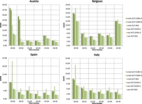
FIGURE 2. $\rho -SWAPE$ values by projection method, time horizon and country.

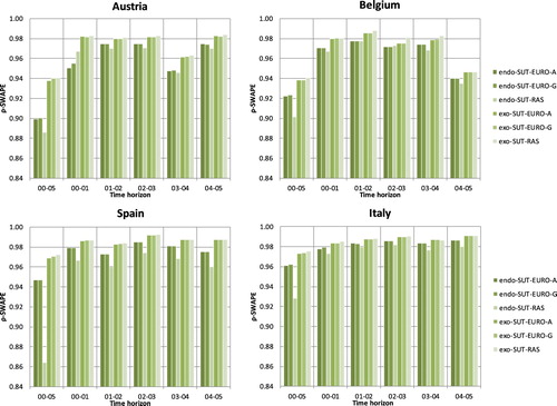
Figures 1 and 2 also show that, for all countries, the use of industry output as exogenous information improves the performance of both methods, i.e. SUT-RAS and SUT-EURO, with respect to their equivalent versions where output by industry is estimated engoenously in the model.

Moreover, in Figure 1 and 2, we can also see that the exo-SUT-RAS method again performed better than the exo-SUT-EURO method for all countries and, as expected, the endo-SUT-EURO performed better than the endo-SUT-RAS method.

Moreover, it can be seen in Figures 1 and 2 that five-year projections usually show a worse performance than one-year projections. This might seem evident: the greater the lapse of time, the more likely it is that the sign-preserving¹² SUT-RAS and SUT-EURO methods do not correctly capture structural changes.

4.2.3 Summary across different elements of the SUTs

We have also conducted an analysis of the performance of the methods across different parts of the SUTs. These results can be briefly summarised in Table 8.

TABLE 8. Goodness-of-fit measure averages by blocks.

Block	WAPE	MASE	WASE	ρ-SWAPE	ρ-PSI	Simil. Ind.
SUT as a whole	6.26	387.24	1.40	0.970	0.970	99.45
Supply table	5.96	114.56	1.74	0.971	0.971	99.47
Intermediate uses matrix	17.08	763.22	4.03	0.918	0.919	97.97
Final Demand matrix	7.00	17.78	0.23	0.964	0.966	99.86

As can be seen in Table 8, regardless of the goodness-of-fit measure considered, the Intermediate Use matrix performed the worst (i.e. it obtained the highest values in the WAPE, MASE and WASE indicators and the lowest values in the normalised ones) while the Final Demand matrix performed the best. The same conclusion holds if we split the same results by methods of projection (see Figure 3).

FIGURE 3. Averages of goodness-of-fit measures by blocks and method of projection. Note: The average values of the MASE indicator have been normalised by division by 30 to make the graph clearer and comparable with the other indicators. Also, the average values of the Similarity Index indicator have been normalised to 100 to match the same range of values as of the other normalised measures.

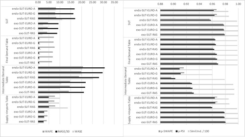
There are various reasons that may explain these results from an empirical point of view. First, the Intermediate Use matrix has the largest number of coefficients (different from zero) to be estimated (ca. 4800 coefficients, depending on the country and year), although the exogenous information available for carrying out the projections has approximately the same dimension as the rest of the blocks. Second, from an economic perspective, we must take into account that structural changes play a major role in the Intermediate Use matrix, leading to large effects more frequently than in the other blocks (technological innovations, relative prices changes, tax and fiscal variations, changes in the structure of imported and domestic inputs, etc.). All these changes imply that it is in the Intermediate Use matrix where greater qualitative difference may arise between the benchmark tables and the projected tables.

Figure 3 shows that the choice preferences across methods remain stable for the different blocks, regardless of the goodness-of-fit measure we consider. The exo-SUT-RAS method is the one with the best outcome for all the blocks considered among the methods with exogenous industry output and the endo-SUT-EURO-G method is the best projection method among those with endogenous industry output. It looks clear again that, when industry output is unknown, the (somehow restrictive) market share assumption of the SUT-EURO methods is superior to the distance-based minimisation process of the SUT-RAS methods. However, when the output by industry is known, the conclusion is exactly the opposite.

Figure 3 also reveals that SUT-EURO-G methods perform better than SUT-EURO-A methods, for both exogenous industry output and endogenous industry output methods. Even though it is not shown in the Figure 3 (for the sake of brevity), if we replicate this analysis splitting results by countries, the fact that the geometric model overcomes the arithmetic model in both situations, exogenous and endogenous industry output, remains valid regardless the country taken into account. The reader can find as supplementary files all the goodness of fit, ranks and results by method, projection horizon, country and block that can be used by the interested reader to easily replicate all the tables and figures presented in this article and check all related findings.

4.2.4 Summary of other interesting findings

To conclude our empirical assessment, we shed light on some specific and remarkable findings that somewhat deviate from the general conclusions drawn so far. They also help us to obtain some additional insights into the strengths and weaknesses of the SUT-EURO and SUT-RAS methods.

Firstly, by taking a closer look at Figure 3, we can see that the errors between exogenous industry output and endogenous industry output methods are very similar for the Final Demand table compared to the rest of the blocks. This is mainly due to the fact that the piece of additional information used in exogenous output by industry methods has only an indirect effect on the estimation of the Final Demand table. As a matter of fact, output by industry interacts in the SUT-RAS and SUT-EURO methods only for improving the estimation of the elements of the Supply and the Intermediate Demand tables. Hence, the effect on the Final Demand (if any) is basically indirect. As long as the domestic and the imported parts of the Intermediate uses table are better estimated (and also the output by-product in the Supply table), the domestic and imported Final Demand elements will be better estimated too. This is an indirect effect in the estimation process that empirically does not add too much information to the estimation of the Final Demand table (Figure 3). In short, the availability of industry output is not significant when the purpose is to estimate the elements in the Final Demand table.

A second interesting feature is that the vector of imports is estimated better by the SUT-RAS methods in all cases (see Table 9). This is mainly due to the fact that imports are estimated in the SUT-EURO methods on the basis of growth rates of GVA by industry while in the SUT-RAS methods they are derived from a more flexible approach (distance minimisation).

TABLE 9. Number of times each method of projection ranks in the i-th position according to combined rank and time horizon projections for imports.

		Ranking
		Five-year projections			One-year projections			Global
	Method	1	2	3	1	2	3	1	2	3
Ranks considering endogenous industry output methods only	endo-SUT-EURO-A	1	1	2	5	6	9	6	7	11
	endo-SUT-EURO-G	1	3		1	15	4	2	18	4
	endo-SUT-RAS	2		2	14		6	16		8
Ranks considering exogenous industry output methods only	exo-SUT-EURO-A			4		10	10		10	14
	exo-SUT-EURO-G		4		3	10	7	3	14	7
	exo-SUT-RAS	4			17	1	2	21	1	2

This feature of the SUT-EURO methods clearly opens the door for future improvements through the use of exogenous information on growth rates of imports (maybe from official trade statistics) instead of GVA growth rates.

One last interesting point is the assessment of endogenous methods concerning the estimation of the output by industry. The output by industry is not available in these methods and must be endogenously estimated. In the endo-SUT-EURO methods, the output by industry is estimated by means of the Leontief quantity model (Dietzenbacher, 1997; Rueda-Cantuche, 2011). In the endo-SUT-RAS method, industry output is estimated by minimising a specific distance function, which measures the distance between the benchmark tables of the base year and the projected tables (Temurshoev et al, 2011).

The results are clear as well on this point and they are shown in Table 10. The logic of economics that substantiates the Leontief quantity model in the SUT-EURO method leads to a better outcome of the output by industry than the one produced by distance minimisation. Furthermore, the geometric version of the SUT-EURO method performs better than its arithmetic version.

TABLE 10. Average goodness-of-fit measures by projection method for the output by industry.

Block	WAPE	MASE	WASE	ρ–SWAPE	ρ–PSI	Simil. Ind.
endo-SUT-EURO-A	5.3	3.8	0.133	0.982	0.976	99.8
endo-SUT-EURO-G	5.1	3.6	0.129	0.982	0.977	98.1
endo-SUT-RAS	5.8	4.1	0.181	0.969	0.970	99.8

5. Conclusions

In this paper, we have introduced new variants of the original SUT-EURO and SUT-RAS methods for updating SUTs and compared them using similar exogenous information, i.e. with and without exogenous industry output data. In addition, these new methods are ready to use and coherent with National Accounts standards, i.e. including changes of valuation concerning taxes less subsidies on products.

For endogenous industry output methods, the information required for the projections year are: (i) GVA by industry; (ii) Final Demand at purchasers’ prices by final use categories; (iii) overall total imports; and (iv) overall total taxes less subsidies on products. For exogenous industry output methods, (v) output by industry should also be available. We have run an empirical assessment of all of these methods against a set of annual SUTs for the years between 2000 and 2005 for Austria, Belgium, Spain and Italy and drawn the following main conclusions:

1. The use of extra information (i.e. industry output) generally improves projected estimates both in the SUT-EURO and SUT-RAS methods. One exception though might be the estimation of the Final Demand matrix with very small differences between endogenous industry output and exogenous output methods.

2. Whenever industry output is available, the SUT-RAS method should be used. Otherwise, the SUT-EURO method should be used instead. This conclusion holds independently of the time horizon, country and element of the SUTs analysed. One exception though is the estimation of the vector of imports, where the SUT-RAS method would be the one to be used in all cases at least while not using other external information on trade statistics to compute the growth rates of imports by industry/product in the SUT-EURO method.

3. When unavailable, total industry output is best estimated by the SUT-EURO method. This might show the superiority of the Leontief quantity model over distance minimisation approaches.

Other interesting but less relevant conclusions are the following:

1. The geometric version of the SUT–EURO methods usually performs better than its arithmetic version.

2. Five-year projections usually perform worse than one-year projections. This might seem logical as the greater the lapse of time, the more likely it is that the sign-preserving SUT-RAS and SUT-EURO methods do not correctly capture structural changes.

3. The Intermediate Use matrix is the part of the SUT framework that is usually worst estimated while the Final Demand matrix is the one that is normally estimated best.

Acknowledgements

We gratefully acknowledge EUROSTAT and the Austrian, Belgian, Italian and Spanish National Statistics Offices for having provided us with their annual estimations for SUTs at basic prices. The results shown here would have not been possible without such information. We also thank the editor and four anonymous referees for their valuable comments and suggestions. The views expressed herein are those of the authors and do not necessarily reflect an official position of the European Commission.

Disclosure statement

No potential conflict of interest was reported by the authors.

Notes

1 For the European Union (EU), according to the European Transmission programme (Annex B of the Council Regulation (EU) No 549/2013 of the European Parliament and of the Council of 21 May 2013) data delivery of SUIOTs should take place 36 months after the reference period.

2 The KRAS method is a generalization of the GRAS method, suitable for cases where exogenous information is conflicting (cfr. Gallego and Lenzen, 2009). When exogenous information is not conflicting, reliability weights are set to one (i.e. all the information available is given the same reliability) and constraints coefficients are 1 or −1, the KRAS method is equivalent to the GRAS method.

3 To our knowledge, only Temurshoev et al. (2011) stated in a footnote (p. 880) a way to include TLS in the SUT-RAS method but without distinguishing between domestic and import uses.

4 Matrices and vectors are given in bold upper (X) and lower case (x), respectively. Scalars are expressed in italics and lower case (x). Vectors are defined by default by column so row vectors are defined by means of the transposition sign (prime) x’. $\mathit{\iota }$ stands for a vector with all elements equal to one. $\stackrel{\mathbf{ˆ}}{\mathit{x}}$ denotes a diagonal matrix with the elements of vector $\mathbf{x}$ placed on its main diagonal and zero otherwise (off-diagonal elements). Subscripts may denote the year or the valuation concept (basic prices, b; purchasers’ prices, p).

5 This is denoted by superscripts in matrices and vectors. Domestic uses are denoted with superscript d and imported uses with superscript m.

6 Our aim is to stick as much as possible to the original SUT-EURO method rather than creating a new model by means of assuming other alternatives such as, for instance, the stability of the product mix instead of the market share.

7 Other options could have been possible, however, according to Eurostat (2008, p. 316), Model D (fixed product sales structures) is favoured against the assumption of fixed industry sales structures which seems to be rather unrealistic. This is also the choice of several European Union countries that compile industry-by-industry SIOTs (Rueda-Cantuche, 2011, p. 26)

8 $\mathbf{O}$ and $\mathbf{0}$ are null matrices and vectors with adequate dimensions.

9 More details on the pros and cons of different measures of goodness of fit can be found in Knudsen and Fotheringham (1986), Makridakis (1993), Butterfield and Mules (1980) and Hyndman and Koehler (2006).

10 An IS = 1 implies that a perfect and direct linear correlation between $X$ and $\tilde{X}$ exists. This is the case when $X=\tilde{X}$ , a perfect match. However, some kind of systematic errors (linear shifts such as $\tilde{X}=X+a$ , or scale transformations $\tilde{X}=a\cdot X$ ) could also lead to an IS = 1. So, for practical purposes, the interpretation of this indicator should be done carefully, since a very good fit could be due to some kind of systematic errors instead of a good fit.

11 Without loss of generality, we do not show the results for the other indicators because they do not provide any new additional information and/or conclusion. All the results are available in a specific Appendix where all the results, figures and tables provided in this article can be reproduced and checked by the reader.

12 For the SUT-EURO method, this is clear because every element of the use table is rescaled by positive column and row factors. As for the supply table, this is also true given the fact that the Supply Table is computed preserving the base-year market shares multiplied by the consistently estimated output by product. The demonstration for the SUT-RAS method can be found in Temurshoev and Timmer (2011, p. 868).

References

- Arto, I., J.M. Rueda-Cantuche and G.P. Peters (2014) Comparing the GTAP-MRIO and WIOD Databases for Carbon Footprint Analysis. Economic Systems Research, 26, 327–353. doi: 10.1080/09535314.2014.939949
- Beutel, J. (2002) The Economic Impact of Objective 1 Interventions for the Period 2000–2006. Report to the Directorate–General for Regional Policies, Konstanz. Available in http://ec.europa.eu/regional_policy/sources/docgener/studies/pdf/objective1/final_report.pdf.
- Beutel, J. (2008) An Input-Output System of Economic Accounts for the EU Member States. Interim Report for Service Contract Number 150830-2007 FISC-D to European Commission. Directorate–General Joint Research Centre. Institute for Prospective Technological Studies.
- Butterfield, M. and T. Mules (1980) A Testing Routine for Evaluating Cell by Cell Accuracy in Short-cut Regional Input-Output Tables. Journal of Regional Science, 20, 293–310. doi: 10.1111/j.1467-9787.1980.tb00648.x
- D’Agostino, R.B. and M.A. Stephens (1986) Goodness of Fit Techniques. New York, Marcel Dekker.
- Dalgaard, E. and C. Gysting (2004) An Algorithm for Balancing Commodity-Flow Systems. Economic Systems Research, 16, 169–190. doi: 10.1080/0953531042000219295
- De Mesnard, L. (2004) Biproportional Methods of Structural Change Analysis: a Typological Survey. Economic Systems Research, 16, 205–230. doi: 10.1080/0953531042000219312
- De Mesnard, L. and R.E. Miller (2006) A Note on Added Information in the RAS Procedure: Re-Examination of Some Evidence. Journal of Regional Science, 46, 517–528. doi: 10.1111/j.1467-9787.2006.00450.x
- Dietzenbacher, E. (1997) In Vindication of the Ghosh Model: A Reinterpretation as a Price Model. Journal of Regional Science, 37, 629–651. doi: 10.1111/0022-4146.00073
- Eurostat (2008) Manual of Supply, Use and Input-Output Tables. Luxembourg, Official Publications of the European Communities.
- Gallego, B. and M. Lenzen (2009) Estimating Generalised Regional Input-Output Systems: A Case Study of Australia. In: M. Ruth and B. Davíðsdóttir (eds.) The Dynamics of Regions and Networks in Industrial Ecosystems, Cheltenham, England, Edward Elgar Publishing 55–82.
- Günlük-Senesen, G. and J.M. Bates (1988) Some Experiments with Methods of Adjusting Unbalanced Data Matrices. Journal of the Royal Statistical Society, Series A, 151, 473–490. doi: 10.2307/2982995
- Hewings, G.J.D. (1969) Regional Input-Output Models Using National Data: The Structure of the West Midlands Economy. The Annals of Regional Science, 3, 179–191. doi: 10.1007/BF01283763
- Hewings, G.J.D. (1977) Evaluating the Possibilities for Exchanging Regional Input-Output Coefficients. Environment and Planning A, 9, 927–944. doi: 10.1068/a090927
- Huang, W., S. Kobayashi and H. Tanji (2008) Updating an Input–Output Matrix with Sign–Preservation: Some Improved Objective Functions and their Solutions. Economic Systems Research, 20, 111–123. doi: 10.1080/09535310801892082
- Hyndman, R.J. and A.B. Koehler (2006) Another Look at Measures of Forecast Accuracy. International Journal of Forecasting, 22, 679–688. doi: 10.1016/j.ijforecast.2006.03.001
- Jackson, R.W. (1998) Regionalizing National Commodity-by-Industry Accounts, Economic Systems Research, 10, 223–238 doi: 10.1080/762947109
- Jackson, R.W. and A.T. Murray (2004) Alternative Input–Output Matrix Updating Formulations, Economic Systems Research, 16, 135–148. doi: 10.1080/0953531042000219268
- Junius, T. and J. Oosterhaven (2003) The Solution of Updating or Regionalizing a Matrix with Both Positive and Negatives Entries. Economic Systems Research, 15, 87–96. doi: 10.1080/0953531032000056954
- Knudsen, D.C. and A.S. Fotheringham (1986) Matrix Comparison, Goodness of Fit and Spatial Interaction Modelling. International Regional Science Review, 10,127–147. doi: 10.1177/016001768601000203
- Kullback, S. and R.A. Leibler (1951) On Information and Sufficiency. The Annals of Mathematical Statistics, 22, 79–86. doi: 10.1214/aoms/1177729694
- Kullback, S. (1959) Information Theory and Statistics. New York, John Wiley and Sons.
- Lahr, M.L. (2001) Reconciling Domestication Techniques, the Notion of Re-exports and Some Comments on Regional Accounting, Economic Systems Research, 13, 165–179 doi: 10.1080/09537320120052443
- Lahr, M. L. and L. de Mesnard (2004) Biproportional Techniques in Input-Output Analysis: Table Updating and Structural Analysis. Economic Systems Research, 16, 115–134. doi: 10.1080/0953531042000219259
- Lemelin, A. (2009) A GRAS Variant Solving for Minimum Information Loss. Economic Systems Research, 21, 399–408. doi: 10.1080/09535311003589310
- Lenzen, M., R. Wood and B. Gallego (2007) Some Comments on the GRAS Method. Economic Systems Research, 19, 461–465. doi: 10.1080/09535310701698613
- Lenzen, M., B. Gallego and R. Wood (2009) Matrix Balancing Under Conflicting Information. Economic Systems Research, 21, 23–44. doi: 10.1080/09535310802688661
- Makridakis, S. (1993) Accuracy Measures: Theoretical and Practical Concerns. International Journal of Forecasting, 1, 111–153. doi: 10.1002/for.3980010202
- Mainar-Causapié, A. et al. (2017) Estimating Regional Social Accounting Matrices to Analyse Rural Development. SORT-Statistics and Operations Research Transactions, 41(2), 319–346.
- Mesnard, L. and R.E. Miller (2006) A Note on Added Information in the RAS Procedure: Reexamination of Some Evidence. Journal of Regional Science, 46(3), 517–528. doi: 10.1111/j.1467-9787.2006.00450.x
- Oosterhaven, J. (2005) GRAS versus Minimizing Absolute and Squared Differences: A Comment. Economic Systems Research, 17, 327–331. doi: 10.1080/09535310500221864
- Polenske, K. R. (1997) Current uses of the RAS Technique: A Critical Review. In: Simonovits, A. and A.E. Steenge (eds.) Proportions, Growth, and Cycles. London, Macmillan, 58–88.
- Rueda-Cantuche, J.M. (2011) The Choice of Type of Input-Output Table Revisited: Moving Towards the use of Supply-use Tables in Impact Analysis. Statistics and Operations Research Transactions (SORT), 35, 21–38.
- Serpell, M.C. (2018) Incorporating Data Quality Improvement into Supply-use Table Balancing. Economic Systems Research, 30, 271–288 doi: 10.1080/09535314.2017.1396962
- Shannon, C.E. (1948a) A Mathematical Theory of Communication. Bell System Technical Bulletin Journal, 27, 379–423. doi: 10.1002/j.1538-7305.1948.tb01338.x
- Shannon, C.E. (1948b) A Mathematical Theory of Communication. Bell System Technical Bulletin Journal, 27, 623–659. doi: 10.1002/j.1538-7305.1948.tb00917.x
- Szyrmer, J. (1989) Trade-off between Error and Information in the RAS Procedure. In: R.E. Miller, K.R. Polenske and A.Z. Rose (eds.) Frontiers of Input-Output Analysis. New York, Oxford University Press.
- Temurshoev, U., C. Webb and N. Yamano (2011) Projection of Supply and Use Tables: Methods and Their Empirical Assessment. Economic Systems Research, 23, 91–123. doi: 10.1080/09535314.2010.534978
- Temurshoev, U. and M.P. Timmer (2011) Joint Estimation of Supply and use Tables. Papers in Regional Science, 90, 863–882. doi: 10.1111/j.1435-5957.2010.00345.x
- Temurshoev, U. (2012) Entropy-based Benchmarking Methods. Research Memorandum GD-122. Groningen Growth and Development Centre. Groningen University. Available in https://www.rug.nl/research/portal/files/15517759/gd122.pdf
- Temurshoev, U., R. E. Miller and M. C. Bouwmeester (2013) A Note on the GRAS Method. Economic Systems Research, 25, 342–361. doi: 10.1080/09535314.2012.746645
- Timmer, M.P., P. Aulin-Ahmavaara and M. Ho (2005) “EUKLEMS Road Map. WP1”. Available in www.euklems.net/workpackages/roadmap_wp1_12-10-2005.pdf
- United Nations (2018) Handbook on Supply, Use and Input-Output Tables with Extensions and Applications. ST/ESA/STAT/SER.F/74/Rev.1, United Nations Publications, New York, 2018. Link: https://unstats.un.org/unsd/nationalaccount/docs/SUT_IOT_HB_wc.pdf