Rents, resources, and multiple technologies; Ricardian mechanisms in input-output modelling

ABSTRACT

To allow for ‘multiple technologies’ to produce a homogeneous output in input–output models, Duchin and Levine [(2011) Sectors may use Multiple Technologies Simultaneously: The Rectangular Choice-of-technology Model with Binding Factor Constraints, Economic Systems Research, 23(3), 281–302] propose an optimization model constrained by primary resources. We show that the Duchin–Levine model contains two different mechanisms by which multiple technologies can arise. If a factor in short supply is shared by the original and the newly entering technology, the output of the original, lower-cost technology will be reduced to make room for the higher-cost technology which is less intensive in that factor. In contrast, if the factor in short supply is technology-specific, a higher-cost technology supplements the original lowest-cost one, which stays fully active. Either mechanism implies a mechanism-specific set of prices, quantities and rents. We relate these results to classical views on comparative advantage, fixed output levels and the origin of rents.

KEYWORDS:

• Multiple technologies
• resource constraints
• scarcity rents
• technology-specific factors
• shared factors

1. Introduction

Within a standard input–output (I–O) model of an economy, each industry produces a homogeneous output using one representative technology. However, in real life multiple co-existing technologies within the same industry are often observed. Duchin and Levine (DL) (2011) ask attention for this fact. They thereby point to the present situation in agricultural or mining-based industries where many technologies can be observed, in one form or another, harvesting food products, or mining metals, minerals, and so on. It therefore may be fruitful to step outside the traditional boundaries of I–O analysis, and focus on situations of ‘multiple technologies’, i.e. situations where individual sectors use more than one technology.¹

DL (2011) pose the question if we can incorporate such situations in an I–O framework. The answer is affirmative. To prove their point, they propose a linear programming I–O model – called the RCOT model ² – of an economy in which sectors can use multiple technologies, each producing the same homogeneous output.³ Factor supply is constrained, which means that a new situation arises if final demand cannot be sustained with the existing supply of the primary factors.⁴ DL (2011) show that in that case an additional technology will enter in one of the sectors, next to the already active technology in that sector, with the new combination minimizing overall factor cost for the economy as a whole. The newly entering technology is more efficient in using the factor at hand, but also more expensive.

In this contribution we shall show that the above-described mechanism is (only) one of two mechanisms by which new technology can enter in a situation where a factor is in short supply. ⁵ These two mechanisms differ significantly in terms of technologies entering and consequences for prices and rents. As we shall show, acknowledging the existence of this second mechanism is essential in understanding modern empirical work. The basic distinction here is whether a factor is shared among multiple technologies or is technology-specific. A shared factor can be used by at least two technologies which may produce the same output, but may also produce different outputs.⁶ In contrast, a technology-specific factor can only be used by the technology to which it is directly linked. If the factor is a shared one, an older technology can be gradually displaced by the newcomer. If, on the other hand, the factor is technology-specific, the older technology stays fully active, but the newcomer takes more and more of the sectoral production for its account until it meets another constraint and a third technology enters in that sector, whereby the second is then fixed at a certain level. As we shall see, the economics of this type of factor can be straightforwardly linked to the classical literature.

The two mechanisms have different implications in particular for the way in which rents originate if final demand increases. In practice these differences may be relevant, since the second mechanism is typically seen in agricultural or mining activities where decreasing fertility or productivity play a dominant role in explaining activities at work.

We also signal another issue. This concerns the point that modellers will have to be aware of the role played by the level of factor (dis)aggregation or detail of the technologies represented in the model. That is, they will have to decide if different qualities of, e.g. metal ores are entered as two different factors, or as two specimen of one –broadly defined– factor. The choices made will determine how the factor input coefficients matrices for the regions or countries involved will need to be specified. This in turn, as we shall show, also determines which technologies will enter (and leave) over time, again for increasing final demand.

The above is relevant for establishing the RCOT model’s position in the range of studies investigating the role of the concept of ‘comparative advantage’ in explaining international trade and trade patterns. The term originates in the World Trade Model (see Duchin, 2005) where countries have (or had) to decide on what to produce in the global context. This is basically Ricardo’s famous example of Portuguese-English trade in wine and cloth (Ricardo, [1817] 1973, Ch. 7). In the abstract one-region version of this world model as discussed in DL (2011), this essentially is reduced to a selection mechanism that selects the technology, or technologies, with the lowest opportunity costs.

Regarding the contents of this paper, in Section 2 we briefly recapitulate the basic RCOT model of DL (2011). In Section 3 we look in more depth at the two different factor types and discuss the impact of the imposed constraint on outputs and rents. For both cases, we include a numerical example to show the differences in outcomes. In Section 4 we discuss factor (dis)aggregation and homogeneity more generally and we show the practical implications of choosing one over another with references to some recent papers in the RCOT tradition. Section 5 presents a further discussion and concludes.

2. The RCOT model basic set-up

Below we shall briefly discuss the RCOT model as proposed by DL (2011). The model is a linear optimization model that extends the standard I–O framework in two ways: sectors can have more than one active technology to produce their (homogeneous) product, and factor supply can be constrained. There are two sets of constraints; one specifying that total demand cannot exceed total production, the other one that total factor use cannot exceed the available quantity of a factor. Factor prices and factor stocks are known and invariable. The primal model minimizes a weighted sum of primary factor inputs (Q for short), the weights being the exogenously given factor prices. The dual maximizes the value of net output corrected for rents (S, for short).

The specifications are as follows:

primal: (1) $\min \mathrm{Q}={\mathit{\pi }}^{\mathrm{\prime }}{\mathbf{F}}^{\ast }{\mathbf{x}}^{\ast }$(1)

subject to: (2) $\left({\mathbf{I}}^{\ast }-{\mathbf{A}}^{\ast }\right){\mathbf{x}}^{\ast }\ge \mathbf{y}$(2) (3) ${\mathbf{F}}^{\ast }{\mathbf{x}}^{\ast }\le \mathbf{f}$(3) (4) ${\mathbf{x}}^{\ast }\ge 0$(4)

The starred matrices I${}^{\ast }$ and A${}^{\ast }$ have dimensions m x n with m ≤ n, and are extensions of the square matrices of, respectively, output and input coefficients of the standard I–O model. Each column of A${}^{\ast }$ represents a technology or activity to produce one of the m commodities being distinguished; the corresponding column of the output coefficients matrix I${}^{\ast }$ tells us which commodity is being produced. The vector x${}^{\ast }$ is the n × 1 vector of (to be determined) activity levels. Vector y represents produced final output and f the vector of maximum supply, per period, of the resources distinguished; dimensions are m × 1 and k × 1, respectively.⁷ Matrix F${}^{\ast }$ has dimension k × n, and is the matrix of input coefficients of the k primary factors. As interpreted here, the vector f represents the maximum available flow of a resource in a given year (or any other time period reflected by the underlying input–output data).

The objective function minimizes the total costs of primary factor inputs, where the 1 × k vector π′ is the vector of exogenously determined factor prices. The product π′F${}^{\ast }$ thus is the 1 × n vector of coefficients of cost weighted factor inputs; in our problem π′F${}^{\ast }$ > 0. We should note that the rows of matrix F${}^{\ast }$ are the (row) vectors of the inputs of the k primary factors in the individual technologies. For the dual problem we have:

dual: (5) $\max S={\mathbf{p}}^{\mathrm{\prime }}\mathbf{y}-{\mathbf{r}}^{\mathrm{\prime }}\mathbf{f}$(5)

subject to: (6) ${\mathbf{p}}^{\mathrm{\prime }}\left({\mathbf{I}}^{\ast }-{\mathbf{A}}^{\ast }\right)-{\mathbf{r}}^{\mathrm{\prime }}{\mathbf{F}}^{\ast }\le {\mathit{\pi }}^{\mathrm{\prime }}{\mathbf{F}}^{\ast }$(6) (7) ${\mathbf{p}}^{\mathrm{\prime }}\ge \mathbf{0}$(7) (8) ${\mathbf{r}}^{\mathrm{\prime }}\ge \mathbf{0}$(8)

Here p′ and r′ are, respectively, the vector of commodity prices of dimensions 1 x m, and the vector of rents, of dimension 1 x k.⁸

To see how the underlying mechanism works, we may start from an initial situation where final demand is such that the factor constraints, as given by (3), are not active. In that case each industry uses only one technology and the set of active technologies is ‘square’, which means that there is one technology active per type of output produced. This result goes back to the so-called non-substitution theorem. The theorem itself, in its most well-known version, is described in contributions assembled in Koopmans (ed., 1951). The economy is visualized in terms of an optimization model with a single scarce factor, the use of which is minimized given exogenous final demand. The basic result is that the set of active technologies stays the same (and the input coefficients square matrix) for shifts in final demand, provided the primary factor is in sufficient supply.⁹

The RCOT model extends this situation in two ways. First, the number of primary factors can be more than one. Secondly, each of these factors can be subject to supply-constraints. The model is used to focus on situations where these constraints become active. DL (2011) enforce these situations by reducing the available quantity of resources. When final demand grows, sooner or later a moment will arrive where the maximum supply of a particular resource will be reached. If final demand grows even further, a new technology – if available – will enter that removes the bottleneck. The new technology is more expensive than the old one, but it allows meeting the increased final demand.

2.1. The model from an empirical point of view

In any case, when using the RCOT framework in an empirical study one should be aware of certain key points that imply the determination of exogenous variables, the addition of external information or the adoption of specific assumptions.¹⁰

First of all, the RCOT model typically deals with choices among alternative technologies, a situation that the standard I-O models, by construction, cannot handle. The RCOT approach thereby can focus on the possibility of describing shifts from one dominant technology to another already existing one. It is also possible to involve technologies the introduction of which can be expected in a reasonable time, but also technologies that are still in the research and development phase. Given that, a most interesting question is how these potentially alternative technologies can be represented in terms of I-O input coefficients and introduced into the RCOT model. The standard procedure is through the use of own survey information or external engineering data. The data, subsequently, must be fit into new coefficients columns that, taken together, reflect a possible present or future situation. In Duchin (2016, pp. 388–389) various formalisms in this context are highlighted to reconcile information from different sources. For new technologies sometimes entirely new coefficients columns must be built. These coefficients then essentially must be obtained from sources such as specialized technological research institutes if the technology is completely new. However, technologies new to a country may also be based on information from another country where this technology already exists (Malik et al., 2014).¹¹

A most important point, and one that we are focused on in this contribution, is the specification of the production factors. As we are going to show in the next sections, the way in which the productive factors are modelled and introduced in the RCOT model has a number of implications. The share of production taken care of by alternative technologies is basically determined by the shape of the F${}^{\ast }$ matrix. In fact we are confronted with a choice. A factor can be introduced as shared by other technologies (thereby assuming perfect mobility of that factor) or as technology-specific (assuming different qualities and uses). The exact specification then would depend on the problem studied and on the nature of the factor. Below we shall start with a numerical illustration employing the Duchin-Levine data, and after that we will show the implications of having a different specification for the production factors.

2.2. Numerical illustration

We first start with the non-constrained case.

The basic data are: ${\mathbf{A}}^{\ast }=\left[\begin{array}{cccccc}0.35& 0.15& 0.23& 0.26& 0.28& 0.24\\ 0.25& 0.22& 0.16& 0.22& 0.21& 0.25\\ 0.20& 0.26& 0.30& 0.31& 0.33& 0.30\end{array}\right]$ The matrix of output coefficients I${}^{\ast }$ shows which technologies produce the same output.¹² ${\mathbf{I}}^{\ast }=\left[\begin{array}{cccccc}1& 0& 0& 0& 0& 0\\ 0& 1& 1& 0& 0& 0\\ 0& 0& 0& 1& 1& 1\end{array}\right]$ Hence, there is one technology available to produce output one, two potential technologies for output two and three potential technologies for output three.

There are two non-produced factors. For these, the relevant input coefficients are given by matrix ${\text{F}}^{\ast }$, ${\mathbf{F}}^{\ast }=\left[\begin{array}{cccccc}2.1& 3.2& 1.9& 1.2& 0.8& 1.4\\ 1.2& 2.2& 1.3& 1.3& 1.1& 1.1\end{array}\right]$ Also given are the final demand vector, $\mathbf{y}=\left[\begin{array}{c}20\\ 25\\ 22\end{array}\right]$ and the vector of factor prices, ${\mathit{\pi }}^{\mathrm{\prime }}=\left[\begin{array}{cc}1& 0.9\end{array}\right]$ f (standing for the maximum supply of the primary factors) will be varied over the exercises.

We shall start with the case where the elements of f are ‘large’.¹³ We then have, actually, the case of no constraints on the primary factors. Straightforward calculation gives $Q=791.814$ and ${\mathbf{x}}^{\ast }=\left[\begin{array}{c}106.331\\ 0\\ 87.328\\ 0\\ 103.678\\ 0\end{array}\right]$ That is, the optimal set consists of three activities. For p′, the vector of commodity prices, we find ${\mathbf{p}}^{\mathrm{\prime }}=\left[\begin{array}{ccc}12.785& 11.280& 11.550\end{array}\right]$ Total primary factor use is given by F${}^{\ast }$x${}^{\ast }$. Using the symbol ϕ for these totals, we obtain $\mathit{\varphi }={\mathbf{F}}^{\ast }{\mathbf{x}}^{\ast }=\left[\begin{array}{c}472.161\\ 355.169\end{array}\right]$

3. Two types of factors

In this section, we look in more detail at the characteristics of the technology that enters in the RCOT model when a production constraint is hit. We thereby assume that the technology that enters was already available, but that it was too costly to operate as long as the already active technologies were able to meet final demand. We focus on two types of factors: case A with shared factors and case B with technology-specific factors. As we shall see, this determines how the additional technology functions.

3.1 Case A: shared factors

A shared factor is a factor that is used by two or more technologies. In case A, we describe a situation in which the additional technology also requires the factor in short supply as input. The new technology produces at higher costs, because it requires more input – directly and/or indirectly – of the intermediate and/or non-constrained factors. However, it uses less of the factor in short supply per unit of the output produced.

The new technology will partially replace the more inefficient lowest-cost technology. This frees up some of the constrained factor that can now be used by the more efficient technology, so that the final demand for the product can be met. Exactly that amount of production will be shifted to this new technology that is required to produce the final demand, while exactly exhausting the available quantity of the factor. The price of the output created with the factor in short supply will increase until it matches the higher cost of the entering technology.

The additional technology that requires a shared factor as input can only enter if it uses the factor more efficiently. The alternative technologies are in this case competing substitutes. However, the scarce resource itself, used by the two technologies, is in essence exactly the same, as it can be interchangeably used by the first production technology or the second one.

An example that fits this setting is the use of a fixed supply of water to produce agricultural output. If water is abundantly available, there is no need to economize on its use and farmers may dig trenches in order to divert water to their crops. However, when water becomes scarce, the farmers may invest in capital-intensive drip irrigation, which allows much more efficient use of the resource.

3.2 A numerical example of case A

This numerical example uses the same values as the example in DL (2011). It focusses on one shared factor in short supply.¹⁴ For these, the relevant input coefficients are given by matrix F^{${}^{\ast }$} above.

Following DL (2011), we now impose a constraint on factor 2 equal to its use in the unconstrained case. So, $\mathbf{f}=\left[\begin{array}{c}1000\\ 355.169\end{array}\right]$ That is, a constraint has entered regarding the use of factor 2, while the use of factor 1 is still unconstrained. Now, if we increase demand for one commodity further, the set of activities consisting of a1, a3 and a5 cannot produce it. However, if there is an additional activity, the entry of which means that the economy can use the second factor more efficiently, then increased final demand can be met. In this case, if demand for commodity 3 increases, activity 6 enters. Calculation gives that increased demand for commodity 3 from 22 to 24 units results in $Q=826.517$ and ${\mathbf{x}}^{\ast }=\left[\begin{array}{c}103.591\\ 0\\ 89.481\\ 0\\ 44.106\\ 60.016\end{array}\right]$ We see that the entry of technology a6 means that the output produced using technology a5 is being reduced. We also find $\mathit{\varphi }={\mathbf{F}}^{\ast }{\mathbf{x}}^{\ast }=\left[\begin{array}{c}506.864\\ 355.169\end{array}\right]$ That is, the use of the first (unconstrained) factor has grown significantly. In fact, a substantial substitution between the two factor inputs has taken place. Also Q has increased, due to the more expensive 6th activity having been activated. For the vector of prices p′ we now obtain ${\mathbf{p}}^{\mathrm{\prime }}=\left[\begin{array}{ccc}18.553& 16.566& 17.351\end{array}\right]$ and for the rents vector, ${\mathbf{r}}^{\mathrm{\prime }}=\left[\begin{array}{cc}0& 1.056\end{array}\right],$ which signals that the second constraint is active.

So, technology 6 has appeared as a consequence of factor scarcity. We should note that it is practically impossible to predict which activity will be activated when the stock of one primary factor runs out due to the indirect production linkages. This means that if, say, one type of labour is fully used up, the number of activities producing steel may increase. We also see that rents are attributed to the factor in short supply, in all activities.

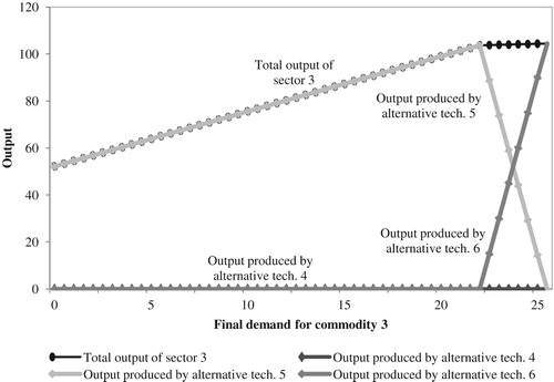
What happens to the output of technology a5 can be observed in Figure 1, where the x-axis measures final demand for commodity 3 and the y-axis output produced by sector 3 (composed by the alternative technologies a4, a5 and a6). Starting from the initial situation where there is no factor scarcity, technology a5’s output increases linearly with the growth in demand for commodity 3 (as said, with all other demand ‘frozen’). The critical point described in the previous paragraph corresponds to a value of 22 for final demand for commodity 3. As soon as final demand reaches 22 for commodity 3, technology a6 enters, and technology a5’s production declines quickly.

FIGURE 1. Output of sector 3 for increasing demand for commodity 3 (shared technologies).

3.3 Case B: technology-specific factors

Although DL (2011) mention that the additional technology can be one related to a technology-specific factor (DL, 2011, p. 285), they do not provide a numerical example for case B. Below we show that the outcomes and the interpretation is distinctly different from case A.

Technology-specific factors are resources that are associated with one technology only. Alternative technologies that alleviate situations in which the technology-specific factor has become scarce may exist, but these rely on the presence of other, possibly closely related, but qualitative different factors. That these technology-specific factors were unused and their related technologies inactive before the situation of short supply occurred implies that these technologies were more costly than the active ones. In this case, the additional technology and related technology-specific factor can be interpreted to be less productive. This ‘diminishing productivity’ concept underlies the analysis of many production processes.

A prominent example is the oil industry, where over time the exploration of oil fields with relative inexpensive technologies in e.g. the Middle-East was complemented by increasingly costly (and dangerous) technologies in some deep sea drilling environments.¹⁵ In this case, the circumstances under which the factor can be recovered imply the use of different extraction technologies with widely diverging costs. Another example of a technology-specific factor is provided by mineral deposits of different qualities. For these factors it is most likely that the associated technology is different, not because of efficiency gains, but directly as a result of the different qualities of the mineral deposits. When the mineral deposit of the best quality is near exhaustion, a more expensive second technology may become economically viable to extract minerals of lesser quality. The additional factors used as input to extract the lower quality deposits are needed so that the output of both technologies will be equal in terms of quality.¹⁶ However, this second technology will not be used to extract the minerals of the best quality as the involved primary factor is intrinsically different. The second technology extracts its inputs from a different deposit and is therefore a different technology, but it produces the same type of output. Hence, in this case we also observe multiple technologies that produce a homogeneous output.

There is also another point of view possible when dealing with constrained technology-specific resources. The one-to-one relation between factor input and scale of operation of the activity in question means that we can discuss the problem of sectors using multiple activities also as a problem of involving (only) processes that are fixed in output capacity. We may think here of many processes in agriculture or mining where output constraints are observed regularly, for example the European milk quota or the OPEC oil quota. Situations where the level of operation of particular production process is fixed are among the most well-known in economic analysis, the discussion often going back to the classical authors (such as Ricardo, [1817]/1973 and Mill, [1909]/1976). Fixing output capacity instead of introducing resource constraints provides a more general model setting, which allows many kinds of production constraints to be incorporated, as long as they are defined in relation to specific technologies. However, by constraining output directly, instead of constraining the supply of a primary resource, the link between a scarce resource and how it limits production is merely implicit and outside the model.

For example, classical economists observed that different qualities of land are used to produce corn. When the available best quality land is not sufficient to satisfy demand for corn, land of inferior quality has to be taken into cultivation. The owners of these inferior quality lands have to employ additional quantities of labour, machinery, fertilizers or other such factors to harvest the same quantity of corn. The additionally required inputs of primary factors make production more costly. However, this cost can be covered by the higher price that is paid for the corn. This also implies that the technologies that can make use of the best quality land receive a rent due to their lower production costs. A well-known quote from Ricardo (1817/1973, Ch. 2, pp. 38–39) captures the basic idea:

The reason then, why raw produce rises in comparative value, is because more labour is employed in the production of the last portion obtained, and not because a rent is paid to the landlord. The value of corn is regulated by the quantity of labour bestowed on its production on that quality of land, or with that portion of capital, which pays no rent. Corn is not high because a rent is paid, but a rent is paid because corn is high; and it has been justly observed, that no reduction would take place in the price of corn, although landlords should forego the whole of their rent. Such a measure would only enable some farmers to live like gentlemen, but would not diminish the quantity of labour necessary to raise raw produce on the least productive land in cultivation.¹⁷

3.4 A numerical example of case B

The DL data (see DL, 2011, Appendix) distinguishes two primary factors, homogeneous labour and capital. Suppose now that there is a third primary factor, which is only used by sector 3. Suppose further that this factor is found in three different ‘grades’ or ‘qualities’ such as different grades of metal ore as described in Section 3. Let us assume that these grades are entered as three separate factors, which means that we have three new factors, each of which is technology-specific. If sector 3 also uses factors 1 and 2 in all its technologies, the corresponding factor input coefficients matrix could look like ${\mathbf{F}}^{\ast }=\left[\begin{array}{cccccc}2.1& 3.2& 1.9& 1.2& 0.8& 2.4\\ 1.2& 2.2& 1.3& 1.3& 1.1& 1.5\\ 0& 0& 0& 1& 0& 0\\ 0& 0& 0& 0& 1& 0\\ 0& 0& 0& 0& 0& 1\end{array}\right]$ To focus the discussion, we shall assume that the first two rows of F${}^{\ast }$ stand for the primary factors labour and capital, used by all technologies and both in sufficient supply. Rows 3, 4 and 5 stand for the inputs of the third primary factor, say land which is available in different fertility types. The input of land is measured in specific units as given in columns 4, 5 and 6.

In this numerical illustration the first two elements of the last column have been increased to reflect additional inputs of labour and machinery. In this case, activity a5 is the technology using the most fertile land, here reflected (compared with alternative technologies a4 and a6) in the lowest inputs of labour and machinery. The fourth technology thereby is less fertile than the fifth one, but more fertile than the sixth, the last one. We shall illustrate the role of the constraints on fertile land, by imposing supply constraints on technologies a4 and a5. Case B, below, gives an illustration.

Adopting the factor input coefficients matrix F${}^{\ast }$ as introduced immediately above, we shall explore in this sub-section the role of technology-specific factors. We hereby adopt the same input coefficients matrix A${}^{\ast }$ as before. As mentioned, we assume that the first two rows of F${}^{\ast }$ stand for the primary factors labour and capital, used by all technologies and both in sufficient supply. We impose two constraints, one on factor 3 (maximum supply 90) and one on factor 4 (maximum supply 60) which are used, exclusively, only by technologies a4 and a5, respectively. Factor 5 is used by a technology, very expensive but available in almost unlimited quantities. Suppose we have, $x_4^{\ast }\le 90$ and $x_5^{\ast }\le 60$

Let us see now what happens if final demand is increasing. We operationalize this by leaving the quantities demanded of commodities 1 and 2 the same (i.e. 22 and 25 units, respectively). However, we let the quantity demanded of commodity 3 increase from 0 with steps of 1 unit. For simplicity, we work with factor prices equal to 1, so π′ = [1 1 1 1 1].

Starting with $\mathbf{y}=\left[\begin{array}{c}20\\ 25\\ 0\end{array}\right]$ we find $Q=589.879$ for the first period (t = 0), and ${\mathbf{x}}^{\ast }=\left[\begin{array}{c}76.438\\ 0\\ 65.553\\ 0\\ 52.169\\ 0\end{array}\right]$ and ${\mathbf{p}}^{\mathrm{\prime }}=\left[\begin{array}{ccc}13.949& 12.435& 13.891\end{array}\right]$ Clearly, there are no rents at this stage. After 100 periods, we have $\mathbf{y}=\left[\begin{array}{c}20\\ 25\\ 100\end{array}\right]$ and outcomes are $\mathbf{Q}=2173.771$ for t = 100, and ${\mathbf{x}}^{\ast }=\left[\begin{array}{c}195.455\\ 0\\ 162.928\\ 90\\ 60\\ 122.385\end{array}\right]$ and ${\mathbf{p}}^{\mathrm{\prime }}=\left[\begin{array}{ccc}15.562& 14.035& 17.133\end{array}\right]$ with positive rents earned, respectively, in activities a4 and a5, ${\mathbf{r}}^{\mathrm{\prime }}=\left[\begin{array}{ccccc}0& 0& 1.318& 1.384& 0\end{array}\right]$ Note that the scarcity rents are not earned by the new, more costly, technology entering with a technology-specific factor. Only the earlier technology already active, which produces the same product, will now earn a rent equal to the difference between the price for the product produced using the more costly method and its own production cost. How the rent is distributed between the owner of the technology and the owner of the technology-specific factor is not given by the model and depends on the bargaining power of both.

Figures 2–4 give the outcomes for the outputs of the 6 technologies, the 3 commodity prices and the 3 activity rents (for the alternative technologies of sector 3) for each period for the trajectory y₃ = 0 to y₃= 100. Recall that the first commodity can be produced with one technology, the second commodity with two technologies (technologies a2 and a3) and the third commodity with three technologies, i.e. technologies a4, a5 and a6.

FIGURE 2. Output of sector 3 for increasing demand for commodity 3 (technology specific).

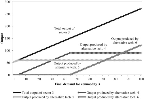
FIGURE 3. Prices of the commodities for increasing demand for commodity 3 (technology-specific).

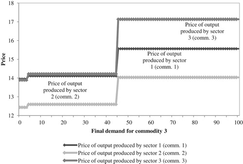
FIGURE 4. Rents obtained by the alternative technologies 3 for increasing demand for commodity 3 (technology-specific).

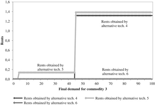
Figure 2 clearly shows that if y₃ = 0, activities a1, a3 and a5 are active. For y₃ = 4, activity a4 enters next to activity a5 in sector 3. Finally, for y₃ = 45, activity a6 enters, so all three possible activities of sector 3 are active.

Figure 3 gives the corresponding prices. We see jumps at the same values of y₃ as in Figure 2. There are two such jumps, which corresponds to the two new activities entering (i.e. activities a4 and a6, at the first and second jump, respectively).

We note that the prices of commodities 1 and 3 are almost the same in the two intervals until y₃ = 45, where first commodity 1 is the more expensive one and then commodity 3. After the last jump (at y₃ = 45) commodity 3 is the most expensive, the intervals between the prices being approximately equal in this case, where the absolute differences between the prices are being caused by accidental similarities in the coefficients matrices.

Figure 4 gives the corresponding rents, earned by activities a4 and a5. First activity a5 starts earning a rent as it was the first to be used in sector 5, and then activity a4. Activity a6, having entered last, earns no rent. The similarities in the rents for activities a4 and a5 are a consequence of numerical properties of the input coefficients matrices.

Finally, we should remark that in realistic cases it may be extremely difficult to predict which technology will enter if demand increases and the supply of a particular factor reaches its limit. Suppose t1 is the original and only technology producing a good g1, reaching, however, its maximum production level. There are two possibilities then to meet increasing final demand (except for unlikely numerical coincidences). Suppose factor j is the factor in short supply. In that case, the newly entering technology (t2) may also use factor j, but less intensively, and we know it will be a more expensive technology. In this case, t2 will enter to satisfy the additional demand by taking over part of the market share of t1.

However, it may quite well be that t2 does not use factor j. Then t1 will stay in place and t2 will provide the needed production increase. However, if demand increases more, also t2 can reach its limit and a third technology (t3) may enter. In that case, it may well be that t3 shares factor j with t1, but uses it less intensively. This then would mean that t3 will acquire part of t1’s market share, thereby not affecting t2. So, also in this case we may recognize the presence of the two mechanisms. However, situations like this may occur quite regularly, and may suggest that the relevance of the distinction between shared and technology specific factors may, in practice, require further attention. In the next section we shall provide additional contextualization.

4. Ideal cases versus complex reality

In this section, we shall continue the points put forward in the last two paragraphs of the previous section. The reason for taking a closer look is that case B above can be seen as an ‘ideal’ case. That is, we are discussing a situation of increasing food production and prime quality land getting scarce. Then lower quality land must be cultivated, and, quite possibly, also land of even lower quality. The entry, successively, of the two lower quality of land technologies then can be directly related to an increase in the demand for food, possibly even for particular types of food. So, here the distinction shared versus technology-specific can be directly linked to classical insights. Probably, however, reality will be more complex and before such direct connections can be further studied, various sensitivity analyses will be asked for, testing the classification assignments. If differences turn out to be substantial, one way forward will be to investigate finer or alternative distinctions. In the sub-sections below we shall explore a number of issues and take a look at empirical work.

4.1. Complex reality

Nonetheless, as we have already briefly seen in the last two paragraphs of the previous section, reality can be more complicated, though, and further contextualization may be required. So let us take a second look at the situation in case B (section 3) and suppose, alternatively, that the factors in rows 4, 5 and 6 are ‘pure’, ‘almost pure’ and ‘less pure’ water respectively, and suppose further that a new competitor for ‘pure water’ arrives on the scene, in this example the flowers industry. This will mean that the I-O input coefficients matrix needs to be enlarged by one sector. The same, clearly, is true for the corresponding F${}^{\ast }$ matrix of factor input coefficients. We might effectively encounter a situation as given (in terms of coefficients) below.

If the newly arrived industry can only use pure water, the situation might be as given by the following F${}^{\ast }$ matrix, ${\mathbf{F}}^{\ast }=\left[\begin{array}{ccccccc}2.1& 3.2& 1.9& 1.2& 0.8& 2.4& 1.0\\ 1.2& 2.2& 1.3& 1.3& 1.1& 1.5& 1.5\\ 0& 0& 0& 1& 0& 0& 0.5\\ 0& 0& 0& 0& 1& 0& 0\\ 0& 0& 0& 0& 0& 1& 0\end{array}\right]$ Because they are now competitors and there is no alternative for the flowers industry, there will be less pure water available for food production and the economy in question, in case of a shortage of pure water, will be forced to satisfy its basic needs now using two qualities of water, pure and less pure. This scenario means that the ‘ideal’ situation as existed before the flowers industry arrived is partly lost. This, in turn, implies that it will be a more complex task to predict at which moment changes will occur.

So, the arrival of the additional industry will be reflected in more complex F${}^{\ast }$ matrices, and using this tool also will be a more complex job. Analogous complexities will show up in employing the associated dual price models regarding the interpretation of changes in rents and prices. Here a confrontation with real-world monitoring of core data will be essential, where, also, the classification of factor qualities and sub-qualities will play a role again. However, before taking a look at empirical work, we shall consider two more situations that characterize the complexity of reality.

4.2. Increasing the critical values

Up to now we have worked with fixed critical values for the factor constraints. That is, the elements of vector f in section 2 were supposed to be constant over time. This, naturally, need not be conform reality. In fact, in many cases activities may be put in place to increase the critical values as given by vector f. Activities like these, however, change the dynamics over time.

To see what happens, let us return to the F${}^{\ast }$ matrix in the previous sub-section. F${}^{\ast }$ depicts a situation where a seventh activity has entered which, next to activity 4, also uses pure water as an input. If the supply of pure water is unaltered over time, we will encounter the situation as described above, i.e. activity 4 will lose part of its share of the market for pure water to the new activity 7.

Suppose now that the clearing of uncultivated lands and water areas results in new values for the maximum supply of pure water. In that case the corresponding elements of the f vector will increase. Now, if the increase in the quantity of pure water being available would be, approximately, of the same order of magnitude as the increase in demand for food and flowers, the outcome may quite well be that activity 4 can expand its output, keeping in tune with increased demand for its product. This might result in a situation where the more expensive activity 5 need not activated. It would also mean that adaptations would be relatively minor.

A scenario like the above may explain part of the results in, e.g. Julia and Duchin (2013). Forest clearing, in that paper, relieves the pressure on the output of certain activities, and prices remain, by and large, the same.

4.3. Factor homogeneity

Above we have discussed a situation of factor homogeneity. That is, the entering industry (flowers) used water of the same quality as the first category of land. In this context an interesting question arises, i.e. how to actually decide if a factor can be qualified as being ‘shared’ by two or more technologies, or whether it is sufficiently ‘distinct’ to be qualified as ‘technology specific’.

So let us again return for a moment to the numerical example of case B and provide additional contextualization. Let us suppose first that modellers do not distinguish between three qualities of land, but only distinguish one type of land. This would mean that activities 4–6 only are different in their inputs of capital or labour, say one being more mechanized than the other ones. Suppose also that final demand for one or more commodities increases. Because the previously distinguished factor 5 is available in unlimited quantities, also the new factor (homogeneous land) is available in unlimited quantities. This means that the situation now is like in case A in section 3; matrix F${}^{\ast }$ would shrink to a 3 × 4 matrix, and all nuances would be lost. The corresponding factor input coefficients matrix could look like ${\mathbf{F}}^{\ast }=\left[\begin{array}{cccc}2.1& 3.2& 1.9& 1.3\\ 1.2& 2.2& 1.3& 1.2\\ 0& 0& 0& 1\end{array}\right]$ where the first two elements of activity 4 are the capital and labour input coefficients of the newly formed, land-based activity.

Suppose now a new activity is distinguished and entered, say (again) flowers production, and that only one activity producing flowers is distinguished. Let us also assume that this new activity also uses ´wateŕ and suppose further that modellers do not agree on the quality of this water. Say, one group prefers to classify the water as ‘pure’, i.e. of the same quality as used in activity 4. However, a second group prefers to classify the water as ‘less pure’, i.e. of the same quality as the water used in activity 5. For the first group the corresponding 5 × 7 factor input coefficients matrix could look like the F^{${}^{\ast }$} matrix as presented in the second paragraph of sub-section 4.1.

However, for the second group it could look like ${\mathbf{F}}^{\ast }=\left[\begin{array}{ccccccc}2.1& 3.2& 1.9& 1.2& 0.8& 2.4& 1.0\\ 1.2& 2.2& 1.3& 1.3& 1.1& 1.5& 1.5\\ 0& 0& 0& 1& 0& 0& 0\\ 0& 0& 0& 0& 1& 0& 0.5\\ 0& 0& 0& 0& 0& 1& 0\end{array}\right]$ In the model without flowers the situation would be as before, we have technology-specific activities and the selection of activities will follow the earlier discussed pattern. However, in the model including flowers the situation is entirely different. Suppose activity 4 is the cheapest one. In that case, if scarcity enters (and competition for pure water begins), the entering flowers producers will cause a reduction in activity 4’s market share and activity 5 will enter to satisfy demand. However, if the situation is like in the F${}^{\ast }$ matrix above, the situation is reversed: activity 4 will keep its place and activity 5 will over time lose its market position.

So, we can encounter, depending on the classification adopted, mixtures of activities the presence of which should be explained following either the technology specific principle or the shared factor principle. This may mean that in practice we are confronted with a very complex situation. The main line may be that we should primarily be looking for technology specific patterns but that the presence of shared factors may disturb this pattern. Our conclusion: classification should be done very carefully. If not, we cannot interpret prices, quantities and rents.

4.4. A look at empirical work

At present several studies have appeared that use the RCOT framework to investigate alternative current scenarios and possible future situations. Empirical applications of the RCOT model so far have focused on alternative technologies in the agricultural sector by distinguishing between rainfed and irrigation techniques, see López-Morales and Duchin (2011), Duchin and López-Morales (2012), Springer and Duchin (2014), López-Morales and Duchin (2015) and Cazcarro et al. (2016), and on the cellulosic biofuel production in the article by Dilekli and Duchin (2015). All contributions specify a different F${}^{\ast }$ matrix depending on the particular topic studied. However, a number of studies, in this way, specify technology specific activities without acknowledging that this imposes a particular type of sectoral behaviour; we shall briefly review these immediately below. In addition, none of these contributions addresses the fundamental question raised in this paper: what will happen when final demand increases?

López-Morales and Duchin (2011) evaluate the impacts of different water policies on withdrawal patterns and the economic costs associated with the change in regional distribution of agriculture through an interregional model of the Mexican economy. Even though the model is not described as a RCOT model, it should be mentioned in this context. Instead of using a rectangular coefficient matrix they implement the model with square matrices that include multiple technological options (non-irrigated agriculture, flood irrigated agriculture, and a mix of drip and sprinkler irrigation technologies). Regarding the way the F${}^{\ast }$ is specified, they considered five factors of production that combines the two frameworks described in the previous sections: labour, capital, non-irrigated land, irrigated land, and blue water.¹⁸ Labour, capital and blue water are shared by the alternatives technologies, while non-irrigated land and irrigated land are technology-specific.

Duchin and López-Morales (2012) can be considered as the first RCOT application. The article specifies two technologies that agriculture can employ; rainfed agriculture and irrigated agriculture. Even though in the paper it is described how the factor requirements and constraints should be modelled using blue and green water (blue water is just used for the irrigated agriculture technology while green water is used for both alternatives), they use the same interregional database as in López-Morales and Duchin (2011) and subsequently the same specification (i.e. involving technology-specific factors).

In a similar line, in Springer and Duchin (2014) a conceptually closely related application is presented, but now for ten regions of the world to address the changes that might be needed to satisfy likely global demand for food by 2050 while constraining water and land resources to be used sustainably. They distinguish nine factors of production: capital, labour, three categories of land (rainfed cropland, irrigated cropland and pastureland), three categories of fossil fuels and water as the ninth factor. So, the agricultural sector consists of two types of crop production and livestock. Water use is shared by all agricultural sectors, the industrial sectors and household demand. In addition, a second technological option is added for the livestock sector, so that it can also use cropland in addition to pastureland. Hence, in this application water is a shared factor for producing crops. Unfortunately, the water and land requirements for the different technologies are not explicitly specified which obscures this important modelling aspect and limits the analysis of the interpretation of the outcomes relative to their modelling choices.

López-Morales and Duchin (2015) tries to refine the results of López-Morales and Duchin (2011) and Duchin and López-Morales (2012) by distinguishing between different water sources and specific conditions for water sustainability. Two scenarios are considered in the analysis: one accounting for the effective supply of water, and the other quantifying the costs of a sustainable supply of water. The same 13 regions as considered in those previous analyses are entered. Those previous studies used the RCOT framework for choosing among three farming technologies, concluding that a more sustainable use of water in Mexico is possible with the existing technologies but that would be associated with an increase in the price of food of 36% higher. In López-Morales and Duchin (2015), distinguishing among different endowments (groundwater or surface water) changes the obtained results and some of the conclusions. The model then considers 13 regions, 15 sectors and 6 factors of production in total (rainfed, irrigated land, surface water, groundwater, labour and capital). The agricultural sector in each region has three alternative technologies: rainfed, irrigated land using water form surface sources, and irrigated land dependent on aquifers. In this paper the specification of the F${}^{\ast }$ matrix is as follows: rainfed is technology specific, while irrigated land, surface water and groundwater is shared by 3 technologies each (one for agriculture, one for manufacturing and the last one for services), as well as labour and capital (shared by the seven different technologies).

To describe cellulosic ethanol production technologies and how the costs of production can be minimized under a set of constraints, Dilekli and Duchin (2015) used a WTM/RCOT model that combines the inter-regional comparative advantage basis with the choice among technologies. The model includes 18 economic sectors, one of which is represented by three alternative technologies (Gasoline, Cellulosic Ethanol from Timber and Cellulosic Ethanol from Waste) and four factors of production (Labour, Capital, Timber and Cellulosic Waste).

In Cazcarro et al. (2016), the World Trade Model is combined with the RCOT framework and applied to estimate the costs of treating wastewater before it can be reused. Using data from GTAP and Aquastat FAO, they distinguish between three categories of water quality – high, medium, and low – and define two water treatment sectors, of which the first withdraws low-quality water and discharges water of medium quality, and the second takes in medium-quality water and converts it to water of high quality. The disaggregation of the sectors in A${}^{\ast }$ and F${}^{\ast }$ is based on engineering information and cost structures from different sources.

As can be seen in the examples provided by the empirical literature, an analysis of the implications of using a technology-specific design of the factors – lacking in the literature – was needed to fully understand the outcomes obtained by the different scenarios applied. The reason is that many of these studies have introduced technology-specific activities without acknowledging that introducing those activities generates a specific dynamics, in particular when these dynamics are entered by asking what will happen if final demand increases. In fact, none of these studies uses (only) shared production factors, as the framework described in Duchin and Levine (2011), but (uses) a combination of mechanisms depending on the subject studied. Summarizing, labour and capital are normally introduced as shared factors (with perfect mobility between technologies and sectors) while other natural resources such as land (irrigated or rainfed) and, in some cases, blue water are treated in these applications as technology-specific. As pointed out, working with technology-specific factors introduces a particular structure that, by itself, is completely understandable. However, when combined with factors which are shared, model outcomes may become difficult to interpret.

5. Discussion and conclusion

Duchin and Levine (2011) (DL) have initiated a fascinating discussion: how to analyse situations of ‘multiple technologies’ in an I-O framework, i.e. how to represent and study a multitude of technologies producing basically the same commodity, as often seen in practice. DL propose that the phenomenon is caused by the fact that increasing resource scarcities induce production to (partially) shift to technologies that are more costly, but less intensive in these scarce factors. The increasing evidence of resource scarcities requires that (1) models developed to analyse scenarios about the future contain factor constraints, (2) that alternative production options need to be specified to substitute or complement the original lowest cost option and that (3) a mechanism is in place to induce a shift towards these alternative options.

As already briefly referred to in the Introduction, the RCOT model can be interpreted conceptually as a one-region version of the World Trade Model (Duchin, 2005), where instead of technologies in different regions, multiple technologies exist within one region. DL show how cheapest but comparatively less efficient technologies can be replaced over time by more expensive technologies that are more efficient in the use of the scarce resources. In this context also the commodity prices and the appearance of rents is explained.

In this paper we have explored this one-region model further because of the presence of a particular complexity that has not been observed up to now. We have shown that to understand which technologies ‘survive’ and which must make room for other ones, the presence of a separate mechanism needs to be acknowledged and given a place in the model. In this context we have shown that situations of ‘multiple technologies’ can be classified in two types, where the difference between the two depends on whether or not the primary factors are shared among multiple technologies. This fact decides about replacement or not, and also about rents, prices, and quantities. In fact, if factors are not shared, they are technology specific. In that case, if scarcity sets in, we see that cheapest but efficient technologies stay around but are accompanied by more expensive and less efficient technologies. This property of the model especially becomes visible for increasing final demand.

This property also helps us in understanding the now available empirical studies. It appears (as we have put forward in section 4.1), that many factors in DL and other studies have been modelled as technology specific (i.e. in the respective F${}^{\ast }$ matrices), and this then is what these studies find, i.e. technology specificity. Therefore, to understand these studies, the presence of this second type of sectoral interconnection should be recognized.

Therefore, a major outcome of our work is that I-O analysts, both theoretically and empirically oriented, will need to consider carefully how they specify and compile the matrix of factor input coefficients (matrix F${}^{\ast }$ above). If the definition of a particular factor (such as water in its various grades of purity) is not finely tuned to the problem at hand, the necessary insight in the structure of the various price and rents determining mechanisms can be completely lost.

As such, the decision on how to model the factor input requirements of an additional technology in the RCOT model has close connections with the choice of the level of disaggregation in supply, use and input-output tables. A single average can be defined for a sector when it is deemed to be homogenous, or it can be disaggregated into more distinct technologies with different intermediate and factor input structures if the information to do so is available. Representing existing technologies in more detail than one homogenous industry allows researchers to analyse shifts in dominant technologies and the related transition trajectories, for example a shift from fossil-fuel based electricity generation to electricity from renewables.

In case of alternative technologies that are not active at the moment, or do not even exist yet, the information is not contained in the input-output table and will need to be incorporated into the coefficient matrices. Both for disaggregation an existing technology from a sector average and for specifying a new technology, information from technical and engineering sources may be needed. The decision on the level of detail in the additional technologies depends on reasonable assumptions regarding homogeneity in relation to the research question at hand and data availability. These assumptions and decisions should be explicitly discussed in each study, given the impact on the results that we have identified in this paper.

Acknowledgments

This paper has benefited significantly from constructive comments by two anonymous referees and by the editor. In addition, we are indebted to Faye Duchin for discussions and helpful suggestions on various specific aspects of the model. Earlier versions of the paper have been presented at the 22nd IIOA conference in Lisbon, Portugal (14–18 July, 2014), the ISEE International Biennial Conference in Reykjavik, Iceland (13–15 August, 2014), and the 23rd IIOA conference in Mexico City, Mexico (22–26 June 2015). The feedback given by conference participants is gratefully acknowledged. The paper presents the authors’ personal opinions and the views expressed should not be attributed to the European Commission or to EDGaR.

Disclosure statement

No potential conflict of interest was reported by the authors.

Notes

1 We shall use the terms ‘sector’ and ‘industry’ interchangeably. A sector/industry is a collection of businesses that produce the same (homogeneous) output. The terms ‘technology’ and ‘activity’ are also used interchangeably. A technology/activity is the process by which an output is produced. Within an input-output table a technology/activity is represented by technical coefficients representing the mix of inputs required to produce a unit of output.

2 The acronym RCOT stands for ‘Rectangular Choice-of-Technology’. The term ‘rectangular refers to the dimension of the data table: the model allows for more technologies (columns of the table) than outputs produced (rows of the table).

3 The RCOT model as introduced by DL (2011) represents a single economy. Duchin and Levine (2012) integrated the RCOT model in the World Trade Model (Duchin, 2005), to extend its scope to multiple regions/economies.

4 We consider the terms ‘factor’ and ‘resource’ to be equivalent. We use these terms to refer to primary factors and resources.

5 We also use the terms ‘mechanisms’ and ‘dynamics’ to be equivalent in this context.

6 DL (2011) refer to the second type of factor as sector specific. To set it clearly apart from a technology-specific activity, we refer to it as a shared factor.

7 We should add that observed scarcity does not need to be a consequence of physical or geological circumstances; scarcity can quite well be an artificial product, brought about by production cartels like OPEC.

8 We pay additional attention to the role of rents further below.

9 For a discussion of a linear programming interpretation, see Lancaster (1969). See also Kurz and Salvadori (1995) for historical background, especially Chapter 1, Section 3.3 and Chapter 5, Section 7.

10 These issues are related to the introduction of the alternative technologies, the computation of the price factors, the endowment available for each factor, the total final demand for the products and, finally, the specification of the production factors.

11 All this requires (Duchin, 2016, p. 388) that the users must place “substantial trust in the multiple judgments and manipulations made by the authors of the global databases” to assure consistency and comparability. One way to earn trust for database builders is to offer full transparency and alternative modelling and data options. This can be done, for example, by offering options for users to insert their own input data or select the modelling alternative that fits their needs best. A database that is set-up with this philosophy in mind is the Australian Industrial Ecology Virtual Laboratory (IELab) developed by Lenzen et al. (2014). This highly automated collaborative research platform facilitates the harmonization of fragmented and misaligned raw data and offers the necessary flexibility to accommodate a range of research questions. The IELab has been specifically developed to bring together different contributors and users, benefitting from the knowledge that each person brings in. The return for specialist contributors consists of the access to a multi-regional input-output database that is equipped with standard tools for analysis.

12 We use the term ‘activities’ as a synonym for ‘alternative technologies’. The activities themselves will be indicated as a1, a2, etc.

13 As discussed in Section 3.2 and example B in DL (2011).

14 This case is discussed in Section 3.3 and example C in DL.

15 For recent illustrations in the oil extraction industries, see Moyo (2012, pp. 54–55).

16 J.S. Mill (Book III, [1909] 1976, Ch. V, par. 3] describes the concept of decreasing productivity in relation to mining and mines of different quality. He follows the same argument; extracting coal, ores or other substances from deeper in the earth requires more expensive tunnelling, transport, air circulation, and additional precautions to produce the same, uniform type of these substances.

17 See further Kurz and Salvadori (1995) Chapter 10, Section 6 for historical background regarding the principle of differential rent and a discussion of Ricardo’s position in a tradition starting from William Petty, François Quesnay and Adam Smith. See also Chapter 12, Section 5 for a discussion of rent concepts in mining, placed in a long-term perspective.

18 Blue water refers to the contents of reservoirs. Precipitation, which is needed for rainfed agriculture is referred to as green water.

References

- Cazcarro, I., A. López-Morales and F. Duchin (2016) The Global Economic Costs of the Need to Treat Polluted Water, Economic Systems Research, 28, 295–314. doi: 10.1080/09535314.2016.1161600
- Dilekli, N. and F. Duchin (2015) Prospects for Cellulosic Biofuel Production in the Northeastern United States, Journal of Industrial Ecology, 20, 120–131. doi: 10.1111/jiec.12291
- Duchin, F. (2005) A World Trade Model based on Comparative Advantage with m Regions, n Goods and k Factors, Economic Systems Research, 17, 141–162. doi: 10.1080/09535310500114903
- Duchin, F. (2016) A Global Case-Study Framework Applied to Water Supply and Sanitation, Journal of Industrial Ecology, 20, 387–395. doi: 10.1111/jiec.12462
- Duchin, F. and S.H. Levine (2011) Sectors May Use Multiple Technologies Simultaneously: The Rectangular Choice-of-Technology Model with Binding Factor Constraints, Economic Systems Research, 23, 281–302. doi: 10.1080/09535314.2011.571238
- Duchin, F. and S.H. Levine (2012) The Rectangular Sector-by-Technology Model: not Every Economy Produces Every Product and Some Products may Rely on Several Technologies Simultaneously, Journal of Economic Structures, 1, 3. doi: 10.1186/2193-2409-1-3
- Duchin, F. and C. López Morales (2012) Do Water-Rich Regions Have a Comparative Advantage in Food Production? Improving the Representation of Water for Agriculture in Economic Models, Economic Systems Research, 24, 371–389. doi: 10.1080/09535314.2012.714746
- Juliá, R. and Duchin, F. (2013) Land Use Change and Global Adaptations to Climate Change, Sustainability, 5, 5442–5459. doi: 10.3390/su5125442
- Koopmans, T.C. (ed.) (1951) Activity Analysis of Production and Allocation. New York, Cowles Monograph 13 John Wiley & Sons.
- Kurz, H.D. and N. Salvadori (1995) Theory of Production: A Long-Period Analysis. Cambridge, Cambridge University Press.
- Lancaster, K. (1969) Mathematical Economics. (3rd ed.) Macmillan, New York.
- Lenzen, M., A. Geschke, T. Wiedmann, J. Lane, N. Anderson, T. Baynes, J. Boland, P. Daniels, C. Dey, J. Fry, M. Hadjikakou, S. Kenway, A. Malik, D. Moran, J. Murray, S. Nettleton, L. Poruschi, C. Reynolds, H. Rowley, J. Ugon, D. Webb and J. West (2014) Compiling and using Input-Output Frameworks through Collaborative Virtual Laboraties, Science of the Total Environment, 485–486, 241–251. doi: 10.1016/j.scitotenv.2014.03.062
- López-Morales, C. and F. Duchin (2011) Policies and Technologies for a Sustainable Use of Water in Mexico: A Scenario Analysis, Economic Systems Research, 23, 387–407. doi: 10.1080/09535314.2011.635138
- López-Morales, C. and F. Duchin (2015) Achieving Water Sustainability: Analyzing Scenarios Restricting Water withdrawals from Surface and Underground Sources with an Inter-Regional Model of the Mexican Economy, Economic Systems Research, 27, 154–171. doi: 10.1080/09535314.2014.980224
- Malik, A., M. Lenzen, R. Neves Ely and E. Dietzenbacher (2014) Simulating the Impact of new Industries on the Economy: The Case of Biorefining in Australia, Ecological Economics, 107, 84–93. doi: 10.1016/j.ecolecon.2014.07.022
- Mill, J.S. ([1909] 1976) Principles of Political Economy with Some of Their Applications to Social Philosophy, new edition 1909, edited by W.J. Ashley. Fairfield, New Jersey, Augustus M. Kelley.
- Moyo, D.F. (2012) Winner Take All; China’s Race for Resources and What It Means for the World. New York, Basic Books.
- Ricardo, D. ([1817] 1973) The Principles of Political Economy and Taxation (Introduction by D. Winch). London, Everyman’s Library.
- Springer, N.P. and F. Duchin (2014) Feeding Nine Billion People Sustainably: Conserving Land and Water Through Shifting Diets and Changes in Technologies, Environmental Science & Technology, 48, 4444–4451. doi: 10.1021/es4051988