Entropy-based Chinese city-level MRIO table framework

Abstract

Cities are pivotal hubs of socioeconomic activities, and consumption in cities contributes to global environmental pressures. Compiling city-level multi-regional input-output (MRIO) tables is challenging due to the scarcity of city-level data. Here we propose an entropy-based framework to construct city-level MRIO tables. We demonstrate the new construction method and present an analysis of the carbon footprint of cities in China's Hebei province. A sensitivity analysis is conducted by introducing a weight reflecting the heterogeneity between city and province data, as an important source of uncertainty is the degree to which cities and provinces have an identical ratio of intermediate demand to total demand. We compare consumption-based emissions generated from the new MRIO to results of the MRIO based on individual city input-output tables. The findings reveal a large discrepancy in consumption-based emissions between the two MRIO tables but this is due to conflicting benchmark data used in the two tables.

KEYWORDS:

• City-level
• MRIO
• China
• maximum-entropy
• consumption-based emissions

1. Introduction

As home to 54% of the global population and as centres of socioeconomic activities, cities are powering consumption and commerce, ultimately accounting for 60% of the global GDP (Moran et al., 2018; United Nations, 2016). However, resources needed to sustain the demands of urban dwellers are increasingly outsourced globally, meaning cities induce environmental and social impacts that are often far beyond urban geographical boundaries (Fry et al., 2018; Wiedmann et al., 2020; Zheng et al., 2020; Zheng, Meng, et al., 2019), for example, carbon emissions (Long et al., 2019; Mi et al., 2019; Moran et al., 2018), water use (Li et al., 2019), and air pollution (Meng et al., 2017). However, most local governments do not have effective tools that would enable them to understand the environmental footprints of their jurisdictions and thus find it difficult to trace spillover effects induced by their economic activities. In climate change mitigation, the spillover effects are interpreted as carbon leakages that are often found in the supply chains at the city level (Wiedmann et al., 2020). Recently, climate coalition groups have been established, such as the C40 Cities Climate Leadership Group, to build climate-friendly cities, with a particular focus on the spillover effects from consumption activities of cities. Despite this growing concern with cities’ carbon footprints, a lack of data on these city carbon footprints hinders the pursuit of sustainability targets.

Multi-region input-output models (MRIOs) have been widely applied as a tool to trace spillover effects through supply chains and to identify regional heterogeneity (Dietzenbacher, Los, et al., 2013; Miller & Blair, 2009; Wang, 2017). Although much effort has been made to construct MRIO tables in the last decade, this has mostly been at the country level (Dietzenbacher, Lenzen, et al., 2013; Haeger, 1975; Lenzen et al., 2012, 2013; Tukker et al., 2013; Wiedmann & Lenzen, 2018) or the subnational level, such as provinces, states or counties (Huang et al., 2021; Mi et al., 2017; Zheng et al., 2020). Without city-level MRIO databases, most studies about city-level spillover effects adopt a downscaling approach derived from national data with locally featured data (e.g. employment and demographic data) in an attempt to capture local heterogeneity and global environmental implications (Chavez & Ramaswami, 2013; Christis et al., 2019; Moran et al., 2018; Zheng, Meng, et al., 2019). Some studies explore consumption heterogeneity by disaggregating final demands using household survey data at the subnational level, but this approach fails to capture heterogeneity in industrial structures (Ivanova et al., 2016; Minx et al., 2013). Other studies adopt the LCA (Life Cycle Assessment) approach based on household consumption data (Jones et al., 2018; Jones & Kammen, 2011; Weber & Matthews, 2008). However, such approaches are limited because they assume that technologies are identical across regions, and because they often do not trace impacts along the complete supply chain (truncation error).

Data availability is a key challenge to city-level MRIO database construction. Only a few cities publish their single region IO table (SRIO table), but detailed inter-city trade data are unavailable in most cases. Impact Analysis for Planning (IMPLAN) (Lindall et al., 2005) and Industrial Ecology Virtual Laboratory (IELab) (Lenzen et al., 2014, 2017) are pioneers in dealing with the data challenge and providing city-level MRIO tables. The former is dedicated to developing a high-resolution MRIO table for the US and Canada, where it employs a doubly constrained gravity model with data from official surveys on interregional commodity flows. The latter attempts to construct a flexible compilation methodology for sub-regional level MRIO tables based on non-survey methods, following the framework of downscaling from national-level tables (Lenzen et al., 2014). The IElab has been widely applied to developing high-resolution MRIO tables for Australia (Lenzen et al., 2014), China (Wang, 2017), Japan (Wakiyama et al., 2020), Indonesia (Faturay et al., 2017), and the US (Faturay et al., 2020).

Unfortunately, the IMPLAN approach requires detailed survey data that are not available in many countries. The IELab largely follows a top-down approach, offering 11 non-survey methods to regionalise national input-output tables, 7 of which are the variants of location quotient (LQ) methods. The Flegg’s LQ is the most frequently adopted method in the IELab. However, there is uncertainty in the method when selecting an appropriate value for an adjustment parameter (δ). The value is often suggested as 0.3 (Flegg et al., 2015), while other studies suggest a lower or higher value than 0.3 (Bonfiglio, 2009; Kowalewksi, 2015). Moreover, top-down approaches (e.g. LQs) can be appropriately applied to non-competitive IO tables (or Type B) where imports are excluded in intermediate and final demand, but non-competitive IO tables are not always available. In contrast to the IELab, the authors have previously employed a bottom-up approach to construct a city-level MRIO table for the Jing-Jin-Ji urban agglomeration in China based on official city-level IO tables of Hebei province, Beijing, and Tianjin (Zheng, Meng, et al., 2019). However, as city SRIO tables are unavailable in most cases, the approach is very limited for other cities.

To overcome the data challenges this paper proposes a feasible non-survey city-level MRIO construction framework without requiring official city-level SRIO tables. The proposed framework combines publicly available data and an entropy model to generate a supply-demand balance for cities, and then links cities by the doubly constrained gravity model based on the principle of maximum entropy. The method is initially tailored to Chinese cities, but can also be applied to other countries providing the data requirements can be met. In the following sections, we first describe the framework and methodology used to compile city-level MRIO tables, from data collection to final construction. We use the 11 cities of Hebei province to demonstrate the method. We calculate their city-level consumption-based carbon emissions and discuss the sensitivity of demand estimates with a weight that reflects heterogeneity in industries between province and city. We then compare results between consumption-based emissions from the MRIO table constructed in this paper and the MRIO table based on city-level SRIO tables.

2. Framework and methodology

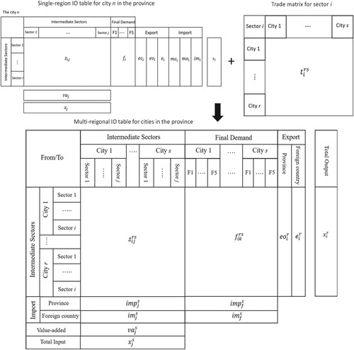
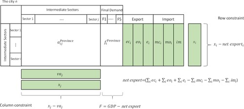
The city-level MRIO table can be regarded as linking city SRIO tables together with trade matrices (Figure 1). The construction of a city-level MRIO table is labour- and time-intensive work, especially for a large country. We first briefly review methods used in the construction of subnational level MRIO tables. Unlike Global MRIO table construction, neither the individual region IO tables nor trade matrices are available in most cases. Non-survey or partial-survey methods are applied to estimating SRIO tables (or intraregional matrix) and trade matrices. At the subnational level, the most adopted methods are location quotient methods (LQs) (Bonfiglio & Chelli, 2008; Kowalewksi, 2015), the commodity balance method (CB) (Miller & Blair, 2009), and the cross-hauling adjusted regionalisation method (CHARM) (Kronenberg, 2012; Többen & Kronenberg, 2015).

FIGURE 1. A brief schematic of city-level MRIO table construction.

LQ-based methods are the most widely applied because of their simplicity. The methods assume that regional technical coefficients are related to national coefficients. LQ-based methods can estimate intermediate and final demands, but treat exports and imports as residuals. As noted, LQ-based methods are more appropriate for Type B tables where imports are excluded from intermediate and final demands, rather than Type A tables where intermediate and final demands include imports. The method is not ideal for China, as China’s SRIO tables are Type A (see SRIO table in Figure 1). Wang applied Flegg’s LQ (one of the LQ-based methods) to China, and yielded the MRIO table of Jing-Jin-Ji urban agglomeration, after converting China’s SRIO tables from Type A to Type B (Wang, 2017). Another problem is in the estimation of final demand, where regional final demand is estimated by using regional value-added to downscale national final demand (Jahn, 2017). This approach may not be reliable since value-added does not reflect local consumption. This assumption can be particularly problematic when imports play an important role in local consumption (Hermannsson, 2016), as they often do for cities.

The commodity balance (CB) method is an alternative to the methods above for Type A tables. Intermediate demands are estimated by multiplying regional outputs with technical coefficients of a given superior table (e.g. national table), while final demand is downscaled from the given table. Net exports are calculated as residuals (total outputs-intermediate demands-final demands). Hence, the CB method cannot yield a full SRIO table, as exports and imports cannot be distinguished. To overcome this shortfall Kronenberg proposed the cross-hauling adjusted regionalisation method (CHARM) which enables the CB method to distinguish exports and imports (Kronenberg, 2009). However, the estimated exports and imports cannot be further distinguished into international and domestic trade. Therefore, CHARM still cannot be used for MRIO table construction that requires detailed trade information (e.g. domestic exports to other regions). Többen and Kronenberg modified the model to estimate domestic trade flows, but the modified model may underestimate cross-hauling (Többen & Kronenberg, 2015), due to its strong assumption that regional cross-hauling shares are identical to the national ones.

Since our aim is to build a city-level MRIO table for China, the modified CHARM is the most suitable option. There are two approaches to applying the modified CHARM. One is the traditional approach as applied in the case of Baden-Württemberg (Többen & Kronenberg, 2015). We could use this approach A with China’s national SRIO table and assume identical cross-hauling shares for all 300+ cities. However, this approach A could be biased because the technical coefficients of 300+ cities may differ sharply from the national technical coefficients. Additionally, it has been noted that CHARM is less reliable when it is applied to small size regions (Flegg et al., 2015).

An alternative approach (approach B) is to construct city-level MRIO tables by province. This is possible since all the provincial SRIO tables of China are available. This approach has the assumption that each city has the same cross-hauling share as its province. However, this approach B assumes that trade with other regions is proportional to the total demand of cities, yet that data on city-level demand is not available for Chinese cities. Therefore, neither of these two approaches is ideal for constructing the city-level MRIO table of China with the given available data.

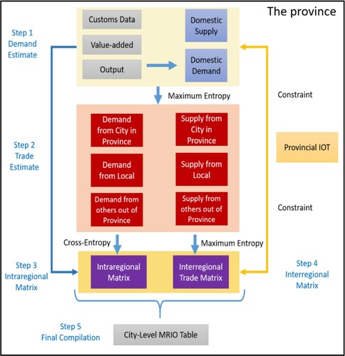
Our framework is rooted in the commodity balance (CB) method, but estimates trade using a maximum entropy model. Since provincial SRIO tables are available for China, we adopt a step-by-step approach to constructing a city-level MRIO table for each province. If one wants to build a full city-level MRIO table for 300+ cities, a nesting approach can be applied to link each city-level MRIO table to its provincial MRIO table (available in China) (Zheng, Meng, et al., 2019). Developing city-level MRIO tables for all cities of a province is the first step in our framework. Next, we elaborate on the framework and procedures. Figure 2 illustrates the compilation steps of the framework, namely: 1. to estimate total demands in each city of a province; 2. to estimate aggregated trade data by sector; 3. to estimate an intraregional matrix and build the SRIO table of each city; 4. to estimate interregional trade flows between cities; 5. To compile the final city-level MRIO table. As shown in Figure 1, SRIO tables for each city are the basis of the MRIO table construction. The key challenge here is how to estimate trade with other cities in the province and trade with other provinces in China to construct SRIO tables.

FIGURE 2. A diagram of the China city-level MRIO table compilation framework.

Entropy theory is the core concept used in our framework. The entropy model is applied to estimating aggregated city trade and interregional trade flow between cities. The notion of entropy is the measure of the degree of the uncertainty (disorder) of an event (David, 1983; Jaynes, 1957; Többen, 2017). When an event has high entropy it means there is high uncertainty about the probability of the event happening, and vice versa. Probability distribution in entropy represents a stage of knowledge, which is different from the objective probability derived from the frequency of outcomes of an event. For an experiment with n possible outcomes, if we have no other information except for the sum of probability for each outcome being equal to 1, the most unbiased estimate is the uniform distribution (1/n), according to Laplace’s principle (Kesavan, 2009). In other words, the uniform distribution of probability maximises the entropy of a system, when no constraints (known information) are imposed on the probability distribution. Once the constraints are imposed, there are many probability distributions of the system consistent with the constraints (known information). Jaynes introduced the Principle of Maximum Entropy: out of all probability distributions consistent with given constraints, the distribution with maximum uncertainty (entropy) should be chosen (Jaynes, 1957). This principle implies that the chosen distribution is characterised by maximal uncertainty about what we do not know, or maximal certainty about what we already know. Therefore, the distribution with maximum entropy offers a least biased estimate that is compatible with given constraints (or incomplete information). Maximum entropy contrasts with minimal entropy which is meant to minimise the entropy distance between the target and a prior distribution (David, 1983; Sargento, 2009). It is worth noting that maximum entropy can be considered as a unique case of minimum cross-entropy, where the prior is evenly distributed (uniform distribution) (Golan et al., 1996), as maximum entropy problems can be converted to minimum cross-entropy problems to minimise the entropy distance between the target and the uniform distribution representing maximum entropy (Többen, 2017).

2.1. Data collection and preparation

The framework developed here has relatively modest data requirements (Table 1). The provincial SRIO table is available for each province, and is treated as the basic benchmark. The provincial SRIO table comprises 42 sectors, including 27 secondary sectors, 14 tertiary sectors and 1 primary sector. For city-level data, the outputs and value-added of all sectors for cities in a province are derived from cities’ statistical yearbooks. The value-added in primary and tertiary sectors can be derived from statistical yearbooks directly, but those of manufacturing sectors may not always be available. Given that the outputs for manufacturing sectors are available we can get the preliminary value-added for each city by multiplying the distribution of the outputs with the total value-added of manufacturing sectors from the provincial SRIO table. Then, we apply RAS to adjust the value-added matrix for manufacturing sectors and tertiary sectors to be compatible with GDP derived from provincial statistical yearbooks.

TABLE 1. The list of data and their sources.

Data	Symbol	Source
Output for sector i in city n	$x_i^n$	City Statistics Yearbook
Value-added for sector i in city n	$v{a}_i^n$	City Statistics Yearbook
Export for sector i in city n	$e_i^n$	China Customs Database
Import for sector i in city n	$i{m}_i^n$	China Customs Database
Provincial technical coefficient between sector i and sector j	$a_{ij}^{\text{province}}$	Province SRIO Table
Provincial final demand for sector i	$f_i^{\text{province}}$	Province SRIO Table
Provincial intermediate demand between sector i and sector j	$z_{ij}^{\text{province}}$	Province SRIO Table
Provincial domestic demand for sector i	$n{d}_i^{\text{province}}$	Province SRIO Table
Provincial foreign export for sector i	$e_i^{\text{province}}$	Province SRIO Table
Provincial foreign import for sector i	$i{m}_i^{\text{province}}$	Province SRIO Table
Provincial domestic export for sector i	$ts{p}_i^{\text{province}}$	Province SRIO Table
Provincial domestic import for sector i	$td{p}_i^{\text{province}}$	Province SRIO Table
Industrial GDP for city n	$gd{p}_{\text{ind}}^n$	Province SRIO Table
Tertiary GDP for city n	$gd{p}_{\text{ter}}^n$	Province SRIO Table
Cost for the shippable sector i	$a{p}_i$	Province MRIO Table
CO2 inventory for sector i of city n	$s_i^n$	CEADS Database

Next, we estimate the outputs of tertiary sectors. Given that the value-added matrix of tertiary sectors is available, we use the distribution of value-added by tertiary sectors by cities to scale up or down the provincial outputs for the tertiary sectors. Each city’s output of each sector is then scaled up or down to be compatible with the provincial output. After all the steps above are taken, the output and value-added of each sector for each city are compatible with the provincial SRIO table. The city-level international trade data (exports and imports) are derived from the China customs database with HS-6 codes and then bridged to the sectoral classification of China SRIO table. All data derived from the statistical documents are then adjusted to be compatible with the sectorial classification of the provincial SRIO table. It should be noted that ‘city' in China refers to an administrative unit at different levels (prefectural level or county level), and cities in this study refer to prefectural-level cities. The city-level in China is equivalent to the NUTS 3 level of the EU classification.

2.2. Step 1: the estimation of supply and demand of cities

The construction begins with the city-level supply and demand estimates for a specific sector i. For a given sector, the supply of a city, which is equal to the city’s output subtracting its foreign export Equation 1, represents the total supply to cities in the country. The demand of a city, which is supposed to be derived from the city-level SRIO table, refers to the total demand of the sector used in the city. Unfortunately, in most cases, there is no city-level SRIO table so domestic demand must be estimated. To estimate the total demand by sector we assume that the ratio of intermediate demand to total demand is identical between a city and its province. It is crucial to note that this assumption implies that the city has as many industries as the province, and is more plausible when a city has a homogenous industry composition as its province, since the provincial ratio only reflects the average level (further discussion in section 3). Since the provincial SRIO table is given we can estimate provisional intermediate demand.

For domestic supply from city n: (1) $\begin{array}{c}{s}_i^n=x_i^n-e_i^n\end{array}$(1) where $x_i^n$ is the total output for sector i in city n, which can be derived from city statistics yearbook;$e_i^n$is the foreign export of sector i in city n, which can be derived from China’s customs database.$s_i^n$ refers to the domestic supply for sector i in city n. (2) $\begin{array}{c}t{d}_i^{\text{province}}=\sum _j{z}_{ij}^{\text{province}}+f_i^{\text{province}}\end{array}$(2)

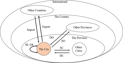
FIGURE 3. The supply-demand flow for the city. The acronyms refer to the demand satisfied by local production (DL), the demand from cities in the province (DC), the demand from other provinces (DO), the export to foreign countries (Export), the supply from a city to itself (SL), the supply from a city to other cities in the province (SC), the supply from a city to other provinces (SO), and the volume of imported goods and services from overseas (Import).

Where $t{d}_i^{\text{province}}$ is the total demand for sector i from the provincial SRIO table, including intermediate demand ($z_{ij}^{\text{province}}$) and final demand ($f_i^{\text{province}}$). For domestic demands for any city n: (3) $\begin{array}{rl}t{d}_i^n& =\left(\frac{{\sum }_j\left(a_{ij}^{\text{province}}\times x_j^n\right)}{\left(\frac{{\sum }_j{z}_{ij}^{\text{province}}}{t{d}_i^{\text{province}}}\right)}\right)\end{array}$(3) (4) $\begin{array}{rl}{d}_i^n& =\frac{t{d}_i^n}{{\sum }_{n}t{d}_i^n}\times n{d}_i^{\text{province}}\end{array}$(4) Where $t{d}_i^n$ is the preliminary total demand for sector i for city n. $\sum _j\left(a_{ij}^{\mathrm{p}\mathrm{r}\mathrm{o}\mathrm{v}\mathrm{i}\mathrm{n}\mathrm{c}\mathrm{e}}\times x_j^n\right)$ represents the sum of preliminary intermediate demand for sector i. $a_{ij}^{\text{province}}$ is the provincial technical coefficient for sector i and j. The denominator $\left(\frac{{\sum }_j{z}_i^{\text{province}}}{t{d}_i^{\text{province}}}\right)$ is the ratio of intermediate demand to total demand in the province, which is assumed to be identical between city and province. $d_i^n$ represents the total demand of city n for sector i constrained by $n{d}_i^{\text{province}}$ which is the provincial domestic demand for sector i, but the aggregation of estimated total demand for each city n in the province should be identical to the total demand of the province. So, we use the proportion of the total demand for each city to distribute the total demand for sector i in the province to different cities.

2.3. Step 2: estimating aggregated trade data by category

For a given sector, domestic demand (D) includes the locally supplied demand (DL), the demand from cities in the province (DC), and the demand from regions outside of the province (DO). Correspondingly, domestic supply (S) consists of the supply to its own city (SL), the supply to cities in the province (SC), and the supply to regions outside of the province (SO). Figure 3 illustrates the supply-demand pool for cities. DL, SL, and DC, SC represent the aggregated intraregional and interregional flows for the given sector, and we adopt a maximum entropy model to estimate these components of supply and demand.

FIGURE 4. The layout of supply and demand matrix for sector i in a given province with n cities.

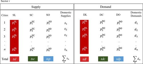
In this case the supply/demand balance serves as an additional constraint. For any sector the supply to local consumers (SL) should be equal to the demand from local consumers (DL), so the red area in the supply and demand block respectively should be equal for the same city (Figure 4). The supply to cities in the province (SC) may not be necessarily equal to the demand from cities in the province (DC), but their aggregated supply and demand should be equal (tsc = tdc or green boxes in Figure 4). This is because all city supply to each other should be the same as all city demand from each other, within a closed provincial boundary. Meanwhile, the supply to other provinces (SO) and the demand from other provinces (DO) are not the same, but their aggregation (tsp and tdp) is derived from the domestic export to other provinces and the domestic import from other provinces in the provincial IO table, respectively. By row, the aggregation of all supplies should be equal to domestic supplies, and the aggregation of all demands should be equal to domestic demands. Mathematically, the maximum entropy (denoted by E) to estimate supply and demand is expressed as: (5) $\begin{array}{c}maxE\left(p_n\right)=-\sum \sum p_n\cdot \ln p_n\end{array}$(5) subject to: $\sum _n{p}_n^{\text{SO}}\times \sum _n{s}_n=tsp$ (the sum of SO of cities constrained by provincial domestic exports in provincial SRIO table) $\sum _n{p}_n^{\text{DO}}\times \sum _n{d}_n=tdp$ (the sum of DO of cities constrained by provincial domestic imports in provincial SRIO table) $p_n^{\text{SL}}\times \sum _n{s}_n=p_n^{\text{DL}}\times \sum _n{d}_n$ (the self-supplied equal to the self-demanded for any city) $\sum _n\left(p_n^{\text{SC}}\times \sum _n{s}_n\right)=\sum _n(p_n^{\text{DC}}\times \sum _n{d}_n)$ (the sum of SC of cities (tsc) equal to the sum of SO of cities (tdc)) $\sum _n{p}_n^{\text{SL}}+\sum _n{p}_n^{\text{SC}}+\sum _n{p}_n^{\text{SO}}=1$ (the sum of probability for the supply is 100%) $\sum _n{p}_n^{\text{DL}}+\sum _n{p}_n^{\text{DC}}+\sum _n{p}_n^{\text{DO}}=1$ (the sum of probability for the demand is 100%) $\left(p_n^{\text{SL}}+p_n^{\text{SC}}+p_n^{\text{SO}}\right)\times \sum _n{s}_n=s_n$ (the sum of the supply for the city constrained by the domestic supply of the city) $\left(p_n^{\text{DL}}+p_n^{\text{DC}}+p_n^{\text{DO}}\right)\times \sum _n{d}_n=d_n$ (the sum of the demand for the city constrained by the domestic demand of the city) $\sum _n\left(\sum _n{s}_n\right)\times p_n^{\text{SL}}+\sum _n\left(\sum _n{s}_n\right)\times p_n^{\text{SC}}+tsp=\sum _n{s}_n$ (the sum of supply to all destination constrained by the total domestic supply of the province) $\sum _n\left(\sum _n{d}_n\right)\times p_n^{\text{DL}}+\sum _n\left(\sum _n{d}_n\right)\times p_n^{\text{DC}}+tdp=\sum _n{d}_n$ (the sum of demand from all destination constrained by the total domestic demand of the province) $p_n^{\text{DL}}>0$ (the probability of self-demand cannot be zero)

In the above, $p_n$ denotes the probability of city n, including the probabilities of supplies ($p_n^{\text{SL}}$,$p_n^{\text{SC}},p_n^{\text{SO}}$) and the probabilities of demands ($p_n^{\text{DL}}$,$p_n^{\text{DC}}$,$p_n^{\text{DO}}$). The terms tsp and tdp represent the domestic exports to other provinces and the domestic imports from other provinces, respectively. These can be derived directly from the provincial IO table. The last constraint ($p_n^{\text{DL}}>0$) states that the probability of local demand cannot be zero, which avoids an unrealistic case where all local demands are met by imports from other regions, and all local supplies go to meet the demands of other regions. In other words, this constraint assumes that the local supply prioritises meeting the local demand. The results of the maximum entropy model are of fundamental importance in the further estimation of intraregional and interregional transaction matrix which are outlined in the following sections.

2.4. Step 3: city IO table regionalisation

After completing the above, we then estimate the intraregional transaction matrix for each city from the provincial IO table. Because the provincial IO table is of type A, the intraregional transaction includes imports, and thus it is not a ‘true' intraregional transaction. We first derive the provincial technical coefficient matrix from the provincial IO table whose element is $a_{ij}^{\text{province}}$. As the provincial technical coefficient matrix reflects the average technical coefficients for all cities in the province, we first assume it is the same as the technical coefficient matrix (${\mathbf{\text{A}}}^n$) of city n in the province as a preliminary estimate for further adjustment. By multiplying the input by the technical coefficient, we can obtain a preliminary matrix for the intermediate demand (${\mathbf{\text{Z}}}^n$) of city n. Second, we derive the distribution of the final demand from the provincial IO table, and assume it is the same as the distribution of the final demand of each city. Then, we calculate the difference between GDP (total value-added) and total net export for each city. The difference should be equal to the final demand. Therefore, the preliminary matrix of the final demand for each city (${\mathbf{\text{F}}}^n$) can be calculated by multiplying the provincial distribution of the final demand by the difference between GDP and total net export for each city. (6) $\begin{array}{rl}{\widehat{\mathbf{\text{Z}}}}^n& =a_{ij}^{\text{province}}\times x_j^n\end{array}$(6) (7) $\begin{array}{rl}netexpor{t}^n& =\sum _{i}e{c}_i^n+\sum _{i}e{o}_i^n+\sum _i{e}_i^n-\sum _{i}m{c}_i^n-\sum _{i}m{o}_i^n-\sum _{i}i{m}_i^n\end{array}$(7) (8) $\begin{array}{rl}{\mathbf{\text{D}}}^{\text{province}}& =\frac{f_i^{\text{province}}}{\sum f_{ik}^{\text{province}}}\end{array}$(8) (9) $\begin{array}{rl}{\widehat{\mathbf{\text{F}}}}^n& ={\mathbf{\text{D}}}^{\text{province}}\times \left(\sum _{j}v{a}_j^n-netexpor{t}^n\right)\end{array}$(9) where ${\widehat{\mathbf{\text{Z}}}}^n$ is the preliminary intermediate transaction matrix from sector i to sector j of city n. The hat accent means the variable is preliminary; $a_{ij}^{\text{province}}$ is the provincial technical coefficient from sector i to sector j; $x_j^n$ and $v{a}_j^n$ represent the total input and the value-added for sector i of city n, respectively; $f_{ik}^{\text{province}}$is the provincial final demand for sector i categorised in segment k (e.g. household consumption), while ${\widehat{\mathbf{\text{F}}}}^n$ is the preliminary final demand matrix for city n; and ${\mathbf{\text{D}}}^{\text{province}}$ is the final demand distribution. $e{c}_i^n$ and $e{o}_i^n$ are the supply of sector i from city n to other cities in the province (SC) and the supply to other provinces in the country (SO), respectively. $m{c}_i^n$ and $m{o}_i^n$ are the demand of sector i for city n from other cities in the province (DC) and the demand from other provinces in the country (DO).

The sum of each row of intermediate demand should be the same as the difference between input and value-added. The sum of each column of intermediate and final demand matrix should be equal to the difference between output and net export. In practice, the preliminary matrix from the provincial proxy does not meet the requirements. The cross-entropy model (CE) is therefore applied to adjusting the matrix to satisfy the constraints utilising prior information that is available from the preliminary matrices $\widehat{\mathbf{\text{Z}}}$ and $\widehat{\mathbf{\text{F}}}$ (Fernandez Vazquez et al., 2015; McDougall, 1999). We combine $\widehat{\mathbf{\text{Z}}}$ and $\widehat{\mathbf{\text{F}}}$ together into a new matrix which is a 42×47 matrix in this case (Figure 5). The entropy between the objective distribution and the prior distribution can be minimised to modify the prior distribution to meet the constraints. The CE approach (denonted by C in Equation 10 generates an outcome equivalent to the widely known RAS, but allows more constraints (Robinson et al., 2001). (10) $\begin{array}{c}minC\left(p_{ij};q_{ij}\right)=\sum _{\text{i}}\sum _{\text{j}}{p}_{ij}\cdot \ln \left(\frac{p_{ij}}{q_{ij}}\right)\end{array}$(10) subject to: $\sum _{\text{i}}\sum _{\text{j}}{p}_{ij}=1;$ $\sum _i{p}_{ij}\times v=cco{l}_j\left(columnconstraint\right).$ $\sum _j{p}_{ij}\times v=cro{w}_i\left(rowconstraint\right).$

FIGURE 5. Regionalisation for the SRIO table of a city. Green blocks refer to known values. The terms ec, eo, mc, and mo are estimated in Equation 5; e and im are derived from the China customs database. The terms x and va are derived from the statistical yearbook of the city.

In the above, the term $q_{ij}$ is the proportion $t_{ij}/\sum _i\sum _j{t}_{ij}$; $p_{ij}$ is the distribution of the matrix T to be estimated; $v$ is the sum of column constraint or row constraint; and $cro{w}_i$ is the row constraint for sector i, which equals output subtracting net export by sector. The term $cco{l}_j$ is the column constraint for sector j, including two parts. The first part is for the constraint of intermediate demand that is equal to input subtracting value-added for sector j, while the second part is for the final demand constraint that is equal to the sum of value-added (or GDP) subtracting net export. Notably, the total column constraint is equal to the total row constraint because the row constraint can be interpreted as input subtracting value-added plus GDP subtracting net export.

The estimated results are the new intermediate transactions and new final demand. Then, we can construct the competitive-type SRIO table of a city. In the following compilation, we then convert the competitive-type IO table into a non-competitive-type table by assuming a fixed proportion of imports and inflows in intermediate and final demand (Miller & Blair, 2009). This process yields an IO table for domestic products and an IO table for imports, where the former is the diagonal of city-level MRIO table, and the latter can be further divided into the IO table for imports from the cities, the IO table for imports from other provinces, and the IO table for imports from overseas. The IO table for imports from the cities is an aggregated IO table for imports from other cities in the province, which is further used to create an off-diagonal matrix. The IO table for imports from other provinces and the IO table for imports from overseas are summed up by row to generate two row vectors: imports from other provinces and foreign countries, respectively.

2.5. Step 4: estimating interregional trade matrix

The most common way to estimate interregional trade flows is by using a gravity model (Riddington et al., 2006; Zhang et al., 2015). However, the lack of observable trade data at the city level makes this method less useful in this study. Therefore, we use the maximum entropy model to estimate interregional trade flows. The maximum entropy approach is equivalent to the doubly constrained gravity model (Wilson, 1967). For sector i, inter-city trade flows between two cities are proportional to total inter-city supply and demand, as well as anti-proportional to transport costs (Többen, 2017). In our case, SC and DC as estimated in Step 2, are treated as the column and row constraint, respectively. Let $t_i^{rs}$ be the trade from city r to s for sector i. PT is the proportion matrix of the trade from city r to s for sector i. For sector i, the entropy measure for inter-city trade flows can be expressed by: (11) $\begin{array}{c}maxH\left(\mathbf{\text{P}}T\right)=-\sum \sum \frac{t_i^{rs}}{{\sum }_r{\sum }_s{t}_i^{rs}}\cdot \ln \left(\frac{t_i^{rs}}{{\sum }_r{\sum }_s{t}_i^{rs}}\right)\end{array}$(11) subject to: $t_i^{rr}=0;$ $\sum _r{t}_i^{rs}=d{c}_i^s;$ $\sum _s{t}_i^{rs}=s{c}_i^r;$

$\sum _r\sum _s{t}_i^{rs}\times d{s}^{rs}\le a{p}_i$ when the shippable product i

In the above, the term $d{c}_i^s$ and $s{c}_i^r$ are the inter-city demand of city s and the supply of city r for sector i, which are the results of Step 2. $d{s}^{rs}$ is the distance between city r and s. The term $a{p}_i$ is the average distance for a shipment of sector i, which is value*km derived from China’s provincial MRIO table. This indicator reflects transport costs, and can be derived from the provincial MRIO table in the absence of inter-city trade statistics. Specifically, we select trade flows between the focal province and its surrounding provinces to estimate the transport costs. For example, in Hebei province, we calculated the average trade flows for each sector between Hebei and its surrounding provinces (e.g. Beijing, Tianjin, Shangdong, Inner Mongolia, Shangxi) as a proxy. It should be noted that the transport costs are only applicable to shippable commodities, while for non-shippable commodities, such as construction and services, we do not set transport costs.

2.6. Step 5: the final construction of a city-level MRIO table

As the city-level SRIO table for each city in the province (Step 3) and the trade matrix for each sector (Step 4) are now available, the next step is to combine the SRIO tables for cities and trade matrices to build the off-diagonal matrix. We utilise a similar approach that has been previously used to construct MRIOs (Feng et al., 2013; Peters et al., 2011). Specifically, we calculate inflow purchase coefficients (IPC) for each sector based on trade matrices, where the IPC for a given commodity is the proportion of all inter-city demand for the commodity that is supplied by each city. Let $ip{c}_i^{rs}$ be the element of $\mathbf{\text{I}}PC$ matrix for each sector i. Thus, $ip{c}_i^{rs}=0.2$ means that for commodity i, 20% of local demands in city s is supplied by city r, so that $\sum _{r}ip{c}_i^{rs}=1$. It is notable that IPC is the opposite of regional purchase coefficients which represent the proportion of local demand for the commodity supplied locally (Lazarus et al., 2002; Lindall et al., 2005).

Let ${\mathbf{\text{Z}}}^{\text{new}}$ and ${\mathbf{\text{F}}}^{\text{new}}$ represent the imported intermediate and final demand matrix, respectively. The off-diagonal matrix for the city-level MRIO table can be estimated by: (12) $\begin{array}{rl}ZM& =\left(IPC\right){\mathbf{\text{Z}}}^{\text{new}}\end{array}$(12) (13) $\begin{array}{rl}FM& =\left(IPC\right){\mathbf{\text{F}}}^{\text{new}}\end{array}$(13) In Equations 12 and 13 $\mathbf{\text{Z}}M$ and $\mathbf{\text{F}}M$ represent the off-diagonal intermediate and final demand matrix in the MRIO table, respectively. Given the diagonal intermediate and final demand in the MRIO table are available (Step 3), we can construct the city-level MRIO table with sectorial value-added, foreign exports, exports to other provinces, foreign imports, and imports from other provinces (see the layout in Figure 1). The city-level MRIO table for the given province is mathematically balanced by row and column, because the provincial SRIO table constrains the compilation at every step. Until this step, we can construct a city-level MRIO table of the focal province. It is crucial to understand that the framework delivers a MRIO table for cities in a given province. If one wants to construct a full city-level MRIO table for all provinces, the step by step approach can be adopted whereby a city-level MRIO table of the province is nested into China’s provincial MRIO table. In other words, trade between cities in different provinces can be constrained by trade between provinces in the provincial MRIO table (Feng et al., 2013; Wang et al., 2017; Zheng, Meng, et al., 2019).

3. The case study of 11 cities in Hebei province

Building on previous work constructing a Hebei city-level MRIO table based on published city-level SRIO tables (Zheng, Meng, et al., 2019; Zheng, Zhang, et al., 2019), we construct a Hebei city-level MRIO table based on the framework developed in this paper and compare the results with our previous work. Here, we call the MRIO table based on the maximum entropy model MRIO-MAX, and call our previous work based on the SRIO tables MRIO-SRIO. To evaluate performance, we use consumption-based carbon emissions as an indicator. Notably, carbon emissions here refer to carbon dioxide emissions, and consumption-based emissions here refer to the areal consumption-based footprint (Heinonen et al., 2020). Consumption-based emissions reflect transboundary emissions between cities, and capture carbon leakages (Arioli et al., 2020; Chen et al., 2017). We choose consumption-based emissions since computing this indicator requires a detailed and accurate MRIO table. We note that developing a city-level MRIO is especially valuable for the Hebei province since it is one of China's main heavy manufacturing regions with huge heterogeneity in industrial structures between cities (Shan et al., 2018).

For validation, we first discuss the validation of assuming that provinces and cities have an identical ratio of intermediate demand to total demand. Next, we compare the consumption-based carbon emissions as computed by the MRIO-MAX and MRIO-SRIO tables. To improve comparability, we use the data from the published SRIO tables for the 11 cities in Hebei to run the entropy model, instead of raw data collected from the city’s statistical yearbooks and customs database. It is worth noting that MRIO-SRIO is based entirely on city-level SRIO tables, and MRIO-MAX is based on the provincial SRIO table. The city-level SRIO tables published by Hebei's statistical agency are not compatible with the provincial SRIO table. Inconsistency between accounts is a longstanding problem that in statistical data published by statistical agencies at different levels (Zheng et al., 2018). Understandably, MRIO tables based on different benchmarks would generate very different results, so the comparison here is meant to evaluate which areas of the resulting model are more reliable and which are less.

3.1. Heterogeneity of weights in city-level consumption-based carbon emissions

One assumption in the framework presented is that cities have an identical ratio of intermediate demand to final demand as their province. We must consider the importance and validity of this assumption. The rationale for using this ratio is that we treat the ratio from the provincial SRIO table as the average for all cities of the province. The ratio reflects the percentage of products used by firms, and is related to the product’s characteristics. For example, products like steel or coal could be more likely to be used by firms as intermediate demand. Hence, the assumption can be reliable for some sectors. Indeed, there are several sectors whose demands are related to the industrial structures of a city, so that the ratio for cities can vary. For example, if a city has many petroleum factories, the city could have a high demand for coal products, and the ratio could be higher than the ratio of the province. In other words, the ratio of the sector for different cities should be different, rather than being identical as assumed. Hence, the next question is: how much would the MRIO table be affected by assigning different ratios?

To answer this question, we carried out a sensitivity analysis on the deviation of the key assumption of the demand estimate. We introduce a random weight matrix ($i\times n$) with the element $w_i^n$ ranging from 0.8–1.2 for sector i in city n, which weights the initial entry within 20%. Mathematically, it can be shown as: (14) $\begin{array}{rl}t{d}_i^{\text{province}}& =\sum _j{z}_{ij}^{\text{province}}+f_i^{\text{province}}\end{array}$(14) (15) $\begin{array}{rl}t{d}_i^n& =\left(\frac{{\sum }_j\left(a_{ij}^{\text{province}}\times x_j^n\right)}{w_i^n\times \left({\sum }_j{z}_{ij}^{\text{province}}/t{d}_i^{\text{province}}\right)}\right)\end{array}$(15) (16) $\begin{array}{rl}d\mathrm{\_}ne{w}_i^n& =\frac{t{d}_i^n}{{\sum }_{n}t{d}_i^n}\times n{d}_i^{\text{province}}\mathrm{\#}\left(16\right)\end{array}$(16) Since the estimated demand for cities ($t{d}_i^n$) is constrained by the provincial domestic demand ($n{d}_i^{\text{province}}$), the weight should be different for each city. It is crucial to understand that the purpose of the weight is to adjust the distribution of preliminary intermediate demand, as the estimated demand would be scaled by the provincial demand Equation 16. The weight has real economic implications, rather than being just a parameter for the sensitivity analysis. However, it is difficult to assign a proper weight, as the weight is boundless and not independent. Higher weight in one city could lead to more provincial demands allocated to the city, and therefore fewer provincial demands would be allocated to other cities.

With the new demand, simulated city-level MRIO tables for Hebei province are generated after 50 runs of the model. We further account for consumption-based carbon emissions based on these MRIO tables. Following Miller and Blair (2009), the basic equation for consumption-based emissions can be expressed as: (17) $\begin{array}{c}C=\mathbf{\text{S}}{\left(\mathbf{\text{I}}-\mathbf{\text{A}}\right)}^{-1}F\end{array}$(17) where $\mathbf{\text{C}}$ represents consumption-based carbon emissions. $\mathbf{\text{S}}$ denotes carbon intensities of all sectors. $\mathbf{\text{A}}$ represents a direct technical coefficient matrix, and $\mathbf{\text{F}}$ denotes final demand. In the simulation, the carbon intensity ($\mathbf{\text{S}}$) is fixed, and is derived from our previous work, while the direct technical coefficient matrix ($\mathbf{\text{A}}$) and the final demand ($\mathbf{\text{F}}$) are changed by different estimated MRIO tables.

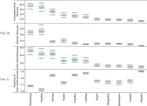
Figure 6 shows discrepancies of consumption-based emissions based on 50 stimulated MRIO tables. Whisker–box plots show the minimum, the $\frac{1}{4}$ quantile, the median, the $\frac{3}{4}$ quantile, and the maximum of the calculated results. Allowing for uncertainty in the distribution of demand, we nevertheless observe that the discrepancies between the maximum and the minimum are not large in terms of absolute value. Large cities are more sensitive to the demand change, such as Shijiazhuang (85.2 vs 61.0 Mt) and Tangshan (92.9 vs 51.4 Mt), but the gap is much narrower in the quartile, indicating that the distribution is more concentrated. For Shijiazhuang and Tangshan, the quartile bounds for Shijiazhuang and Tangshan are 79.8 vs 71.3 Mt and 75.6 vs 63.9 Mt, respectively. The results for small cities show less deviation, indicating relatively higher stability. Trade-related emissions are more sensitive to the demand change than are domestic emissions. Moreover, the proportion of trade-related emissions in consumption-based emissions is stable for all simulated MRIO tables, with the gap between the maximum and the minimum ranging from 2% (Hengshui) to 9% (Qinhuangdao). The relatively stable outcome may indicate less sensitivity to heterogeneity in industries between city and province.

FIGURE 6. The deviation of consumption-based emissions from the sensitivity analysis.

3.2. Comparison with the previous study of 11 cities of Hebei province

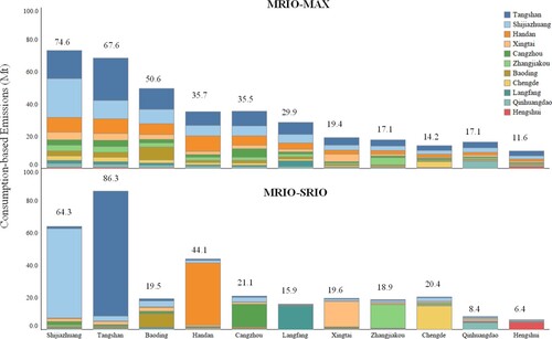
We compared the consumption-based carbon emissions based on MRIO-MAX and MRIO-SRIO. The results show large discrepancies in consumption-based emissions between the MRIO tables (Figure 7). Consumption-based emissions in MRIO-MAX are 373.4 Mt in total, while only 325.0 Mt for MRIO-SRIO. In MRIO-MAX, Shijiazhuang has the largest consumption-based emissions (74.5 Mt), followed by Tangshan (67.6 Mt) and Baoding (50.6 Mt), while in MRIO-SRIO, Tangshan is with the highest consumption-based emissions (86.3 Mt), followed by Shijiazhuang (64.3 Mt) and Handan (44.1 Mt). We then divide the consumption-based emissions into (a) local emissions representing emissions embodied in products made and used locally, and (b) trade-related emissions representing emissions embodied in trade from other cities. Local emissions take a predominant share based on MRIO-SRIO, ranging from 43% to 90% of their total consumption-based emissions. This is particularly high for cities with heavy industries, such as Tangshan (90%), Handan (87%), and Shijiazhuang (86%). The large share of local emissions implies that the demands of the cities are largely met internally. It is not surprising that their local emissions are much higher than the imported emissions, as carbon intensities in these cities are higher than those of other cities. In contrast, the share of local emissions declines significantly in MRIO-MAX. For example, the local shares of consumption-based emissions in Shijiazhuang, Tangshan, and Handan are 32%, 38%, and 27%, respectively. Accordingly, trade-related emissions are much larger in MRIO-MAX, where the trade-related shares of all cities are ranged from 60% to 90% of their consumption-based emissions. The share is particularly high for small-sized cities such as Hengshui and Langfang.

FIGURE 7. Consumption-based emissions in MRIO-MAX and MRIO-SRIO.

It is clear that MRIO-SRIO underestimates trade-related emissions, and hence overestimates domestic emissions. The reason behind the underestimation is the incompatibility between the city SRIO tables and the provincial SRIO table. The former is the benchmark for MRIO-SRIO, while the latter is the benchmark for MRIO-MAX. Table 2 indicates differences in the benchmark between the two tables. Self-supplied demands for cities refer to products made and used in the city (DL in Figure 4). However, in the provincial SRIO table, self-supplied demands for the province include not only products self-supplied to cities (DL), but also products made in one city and used in other cities of the same province (DC in Figure 4). Therefore, the self-supplied demand calculated from city SRIO tables should be smaller than that reported by the provincial SRIO table, but we find contradictory data in many sectors. The sum of self-supplied demands for all 11 cities is higher than self-supplied demands for Hebei province. In the city SRIO tables, the imports are divided into domestic imports and foreign imports. The former contains imports from other cities in Hebei province (DC) and imports from other provinces (DO), while domestically supplied demand for the province includes imports from other provinces (DO). The sum of domestically supplied demand for cities should be larger than that for the province as inter-city trade is normally much larger than the trade between the city and other provinces. However, 10 sectors have their domestically supplied demand in cities smaller than at the province level. In foreign imports, the sum of supplied demand from the city SRIO tables is much smaller than from the provincial SRIO table, indicating that the demand of cities is largely met domestically rather than by foreign imports.

TABLE 2. Benchmark comparison between the sum of city SRIO tables and the provincial SRIO table of Hebei.

	City	Province		City	Province		City	Province
	SL	SL + SC	Ratio	DC + DO	DO	Ratio	Foreign Import	Foreign Import	Ratio
S1	390.5	363.1	1.1	60.3	80.3	0.8	7.0	80.3	0.19
S2	119.2	218.2	0.6	146.4	63.1	2.3	8.3	63.1	0.13
S3	25.8	35.1	0.7	38.7	89.1	0.4	1.0	89.1	0.01
S4	269.8	407.6	0.7	56.3	6.8	8.2	68.6	6.8	10.04
S5	15.4	28.8	0.5	47.9	29.4	1.6	0.2	29.4	0.01
S6	229.0	212.4	1.1	91.6	20.8	4.4	5.5	20.8	0.26
S7	109.7	59.2	1.9	29.8	2.6	11.6	1.6	2.6	0.63
S8	56.8	63.8	0.9	35.2	4.4	8.1	0.8	4.4	0.19
S9	21.9	31.8	0.7	111.6	17.0	6.6	10.1	17.0	0.59
S10	92.2	91.8	1.0	27.5	16.9	1.6	1.3	16.9	0.08
S11	212.5	203.6	1.0	123.4	69.6	1.8	0.9	69.6	0.01
S12	268.6	345.7	0.8	176.6	77.5	2.3	9.1	77.5	0.12
S13	99.1	147.3	0.7	70.6	5.2	13.6	1.7	5.2	0.32
S14	703.8	801.0	0.9	417.2	78.3	5.3	21.3	78.3	0.27
S15	196.2	211.1	0.9	38.1	0.0	829.7	0.9	0.0	20.28
S16	116.0	105.4	1.1	65.6	44.2	1.5	4.1	44.2	0.09
S17	86.0	79.4	1.1	79.3	14.2	5.6	2.6	14.2	0.18
S18	113.0	95.3	1.2	43.8	28.2	1.6	3.1	28.2	0.11
S19	66.3	140.8	0.5	51.8	26.2	2.0	1.3	26.2	0.05
S20	24.7	24.2	1.0	43.7	51.0	0.9	0.8	51.0	0.02
S21	5.5	5.8	0.9	8.8	4.9	1.8	0.7	4.9	0.14
S22	2.5	3.2	0.8	38.3	16.3	2.4	0.1	16.3	0.01
S23	12.9	20.6	0.6	21.8	4.7	4.7	1.0	4.7	0.21
S24	7.1	22.0	0.3	81.4	1.2	68.8	1.0	1.2	0.85
S25	243.3	258.0	0.9	92.9	93.6	0.9	0.0	93.6	0.00
S26	11.5	10.2	1.1	8.2	1.3	6.1	0.0	1.3	0.00
S27	4.0	4.2	0.9	9.7	17.0	0.6	0.0	17.0	0.00
S28	522.7	556.0	0.9	252.2	592.3	0.4	6.2	592.3	0.01
S29	134.8	133.1	1.0	25.5	15.4	1.7	0.8	15.4	0.05
S30	296.3	307.8	0.9	58.2	73.6	0.8	0.5	73.6	0.01
S31	80.5	73.3	1.1	0.6	0.6	1.0	0.0	0.6	0.00
S32	49.5	37.4	1.3	11.2	7.8	1.4	0.0	7.8	0.00
S33	145.9	170.0	0.8	60.3	140.2	0.4	0.0	140.2	0.00
S34	107.9	125.4	0.9	12.2	11.0	1.1	0.0	11.0	0.00
S35	62.5	48.1	1.3	57.5	15.9	3.6	0.1	15.9	0.01
S36	18.9	61.3	0.3	6.3	3.4	1.8	0.0	3.4	0.01
S37	8.7	8.5	1.0	4.3	19.1	0.2	0.0	19.1	0.00
S38	75.4	74.4	1.0	13.4	8.7	1.5	0.0	8.7	0.00
S39	75.2	71.0	1.1	7.1	0.4	19.4	0.0	0.4	0.14
S40	64.1	67.9	0.9	13.2	4.6	2.9	0.0	4.6	0.00
S41	11.2	13.0	0.9	2.4	8.3	0.3	0.0	8.3	0.00
S42	94.6	109.1	0.9	6.3	0.0	182.5	0.1	0.0	2.27

Unit: 1 billion RMB

Bold numbers refer to anomalies

These differences might suggest that MRIO-SRIO overestimates the self-supplied demand. The self-supplied demand is the diagonal part in the MRIO table. The overestimation explains why the local emissions based on MRIO-SRIO are so large. Given the significant difference between the two estimates, one may wonder which MRIO table is more precise. In the absence of other official benchmarks, this question cannot be answered directly, but it is crucial to note that the results from MRIO-MAX are compatible with other studies for global cities. Our study shows the outsourced emissions ranged from 66% to 90% of their consumption-based emissions for 11 cities, and supports the notion that trade-related emissions make up significant parts of consumption-based emissions (Wiedmann et al., 2020). In C40 cities, about 85% of their consumption-based emissions are found to be outsourced for C40 cities (C40 Cities, 2019).

4. Discussion and conclusion

This study explored a method of constructing a city-level MRIO table based on entropy theory. The method is rooted in the commodity balance method, and therefore is suitable for Type A IO tables. The framework overcomes the major challenge of missing city-level SRIO tables. Given that data required are publicly accessible the framework can substantially reduce the data requirements for the construction of a city-level MRIO table. The maximum entropy model is used to estimate disaggregated supplies and demands under a set of constraints that are in line with statistical data and the SRIO table of the focal province. Therefore, the MRIO table is in accordance with benchmarks such as the provincial SRIO table, statistical data for cities, and customs data.

To validate the method we first use Hebei province as a case study and conduct a sensitivity analysis of the MRIO table built using the presented method. We introduce a weight to adjust the initial distribution of estimated demand at the city level. The results show the relative stability of our assumptions in estimating consumption-based emissions for each city, and thus suggest there is less sensitivity when using potential weights to improve the demand estimate. On the contrary, we argue that the weight can improve the performance of the model, especially in a province with huge heterogeneity. However, the question remains of how to determine the proper weight. The assignment of a proper weight needs to be better explored in future research. Second, we compared the consumption-based emissions computed using the MRIO table developed here with a corresponding city-level MRIO table we developed in previous work. Large discrepancies in consumption-based emissions are found between the two tables. The difference is rooted in the incompatibility of benchmarks used for MRIO-SRIO and MRIO-MAX. In the former, the benchmark is the city-level SRIO tables, while the latter is based on the provincial SRIO table. This reflects the fact that official statistics at the city level do not concorde with official published statistics at the province level. The results of comparing two benchmarks show a clear data conflict. The city-level SRIO tables indicate higher self-supplied demands, leading to significant domestic emissions. Previous work has indicated that the choice of raw data and the method of compilation are the main factors that lead to major divergences between the results of different MRIO tables (Qu et al., 2020; Wood et al., 2019). In the field of MRIO table construction, many studies highlight the uncertainty of MRIO tables, but their raw data going into the global country-level MRIOs are almost the same (Arto et al., 2014; Owen et al., 2014; Wood et al., 2019). In our case, it is hard to separate the uncertainty introduced by raw data (different benchmarks) and by methods. We argue that the uncertainty originating from different benchmarks could be much larger than that generated by different methods, as the huge gap between benchmarks (especially in the foreign trade data) conflicts with the supply-demand relationships. In other words, inconsistent benchmarks illustrate very different economies. Given the lack of other official data to justify accuracy, we compare our results with the consumption-based emissions of the C40 cities, and find that our work is in line with the C40 study (C40 Cities, 2019), justifying our claim that the method proposed in this paper can generate an acceptable estimate.

The framework can be implemented not only in China, but also in any country with available sectoral output, value-added, and city-level customs data. The framework can be also implemented at the regional level. The city-level MRIO table for 309 cities has numerous policy implications in terms of both economic growth and environmental conservation. For example, China has launched a series of policies to reduce huge regional disparity, such as ‘China Western Development', ‘Rising in the Central region', and ‘Revitalization of the Northeast provinces', but it is still unclear how the economic growth in rich coastal cities contributes to the growth of poor cities (e.g. GDP or jobs). The dataset is a critical tool to quantify economic linkages between cities, and identifies key cities as well as key sectors. Such quantified linkages between cities can inform the State Council's proposals for economic collaboration between cities and the impact evaluation of economic policies or political events on different cities throughout supply chains. For example, the State Council can evaluate how China’s economic transition in the post-financial crisis affected various, how economic or employment costs varied for each city during the US-Sino trade war, or how industrial and trade structure changed for each city after the Covid-19 pandemic. In the context of climate change, the city-level MRIO table can track how climate risks are distributed among cities and identify which cities are more exposed to, or create, supply chain risk. A recent study measuring the economic and health costs of the California wildfires in 2018 offers a good example of how high-resolution MRIO tables can evaluate the hidden costs of natural disasters (Wang et al., 2020). Hidden costs can not only guide city councils in conducting precautionary actions and comprehensively assessing potential damages, but also offer crucial data to private sectors, such as insurance or real estate companies. Furthermore, China has pledged carbon neutrality by 2060, and cities are major components in this massive mitigation project. The city-level MRIO table can promote city-level consumption-based emission inventories, quantify mitigation responsibilities, and highlight mitigation hotspots. The city-level MRIO dataset can also enable calculating emissions embodied in trade, thereby providing a quantitative tool to help establish city-level carbon markets.

Acknowledgement

We also acknowledge the editor and referees for their time and constructive suggestions. We especially thank the patience and constructive comments from Prof. Manfred Lenzen. We also thank the 8th Edition of the International School of Input-Output Analysis (ISIOA) at 26th International Input-Output (IO) Conference for inspiration.

Disclosure statement

No potential conflict of interest was reported by the author(s).

Additional information

Funding

This work was supported by National Natural Science Foundation of China (72091514, 41921005), the UK Natural Environment Research Council (NE/P019900/1), the Norwegian Research Council (287690/F20), China Scholarship Council (CSC) (No. 201606510016).

References

- Arioli, M. S., D’Agosto, M. d. A., Amaral, F. G., & Cybis, H. B. B. (2020). The evolution of city-scale GHG emissions inventory methods: A systematic review. Environmental Impact Assessment Review, 80, 106316. https://doi.org/10.1016/j.eiar.2019.106316
- Arto, I., Rueda-Cantuche, J. M., & Peters, G. P. (2014). Comparing the GTAP-MRIO and wiod databases for carbon footprint analysis. Economic Systems Research, https://doi.org/10.1080/09535314.2014.939949
- Bonfiglio, A. (2009). On the parameterization of techniques for representing regional economic structures. Economic Systems Research, 21(2), 115–127. https://doi.org/10.1080/09535310902995727
- Bonfiglio, A., & Chelli, F. (2008). Assessing the behaviour of non-survey methods for constructing regional input-output tables through a Monte Carlo simulation. Economic Systems Research, 20(3), 243–258. https://doi.org/10.1080/09535310802344315
- C40 Cities. (2019). Future of Urban Consumption in a 1.5°C World. https://www.c40.org/consumption.
- Chavez, A., & Ramaswami, A. (2013). Articulating a trans-boundary infrastructure supply chain greenhouse gas emission footprint for cities: Mathematical relationships and policy relevance. Energy Policy, 54, 376–384. https://doi.org/10.1016/j.enpol.2012.10.037
- Chen, G., Hadjikakou, M., & Wiedmann, T. (2017). Urban carbon transformations: Unravelling spatial and inter-sectoral linkages for key city industries based on multi-region input–output analysis. Journal of Cleaner Production, 163, 224–240. https://doi.org/10.1016/j.jclepro.2016.04.046
- Christis, M., Athanassiadis, A., & Vercalsteren, A. (2019). Implementation at a city level of circular economy strategies and climate change mitigation – the case of Brussels. Journal of Cleaner Production, 218, 511–520. https://doi.org/10.1016/j.jclepro.2019.01.180
- David, B. (1983). Spatial analysis of interacting economies. Kluwer Nijhoff Publishing.
- Dietzenbacher, E., Lenzen, M., Los, B., Guan, D., Lahr, M. L., Sancho, F., Suh, S., & Yang, C. (2013). Input-output analysis: The next 25 years. Economic Systems Research, 25(4), 369–389. https://doi.org/10.1080/09535314.2013.846902
- Dietzenbacher, E., Los, B., Stehrer, R., Timmer, M., & de Vries, G. (2013). The construction of world input-output tables in the WIOD project. Economic Systems Research, 25(1), 71–98. https://doi.org/10.1080/09535314.2012.761180
- Faturay, F., Lenzen, M., & Nugraha, K. (2017). A new sub-national multi-region input–output database for Indonesia. Economic Systems Research, 29(2), 234–251. https://doi.org/10.1080/09535314.2017.1304361
- Faturay, F., Vunnava, V. S. G., Lenzen, M., & Singh, S. (2020). Using a new USA multi-region input output (MRIO) model for assessing economic and energy impacts of wind energy expansion in USA. Applied Energy, 261(1), 114141. https://doi.org/10.1016/j.apenergy.2019.114141
- Feng, K., Davis, S. J., Sun, L., Li, X., Guan, D., Liu, W., Liu, Z., & Hubacek, K. (2013). Outsourcing CO2 within China. Proceedings of the National Academy of Sciences, 110(28), 11654–11659. https://doi.org/10.1073/pnas.1219918110
- Fernandez Vazquez, E., Hewings, G. J. D., & Ramos Carvajal, C. (2015). Adjustment of input–output tables from two initial matrices. Economic Systems Research, 27(3), 345–361. https://doi.org/10.1080/09535314.2015.1007839
- Flegg, A. T., Huang, Y., & Tohmo, T. (2015). Using charm to adjust for cross-hauling: The case of the province of Hubei. China. Economic Systems Research, 27(3), 391–413. https://doi.org/10.1080/09535314.2015.1043516
- Fry, J., Lenzen, M., Jin, Y., Wakiyama, T., Baynes, T., Wiedmann, T., Malik, A., Chen, G., Wang, Y., Geschke, A., & Schandl, H. (2018). Assessing carbon footprints of cities under limited information. Journal of Cleaner Production, 176, 1254–1270. https://doi.org/10.1016/j.jclepro.2017.11.073
- Golan, A., Judge, G., & Karp, L. (1996). A maximum entropy approach to estimation and inference in dynamic models or counting fish in the sea using maximum entropy. Journal of Economic Dynamics and Control, 20(4), 559–582. https://doi.org/10.1016/0165-1889(95)00864-0
- Haeger, J. W. (1975). Crisis and prosperity in sung China. University of Arizona Press.
- Heinonen, J., Ottelin, J., Ala-Mantila, S., Wiedmann, T., Clarke, J., & Junnila, S. (2020). Spatial consumption-based carbon footprint assessments - A review of recent developments in the field. Journal of Cleaner Production, 256, 120335. https://doi.org/10.1016/j.jclepro.2020.120335
- Hermannsson, K. (2016). Beyond intermediates: The role of consumption and commuting in the construction of local input–output tables. Spatial Economic Analysis, 11(3), 315–339. https://doi.org/10.1080/17421772.2016.1177194
- Huang, Q., Zheng, H., Li, J., Meng, J., Liu, Y., Wang, Z., Zhang, N., Li, Y., & Guan, D. (2021). Heterogeneity of consumption–based carbon emissions and driving forces in Indian states. Advances in Applied Energy, 100039. 10.1016/j.adapen.2021.100039
- Ivanova, D., Stadler, K., Steen-Olsen, K., Wood, R., Vita, G., Tukker, A., & Hertwich, E. G. (2016). environmental impact assessment of household consumption. Journal of Industrial Ecology, 20(3), 526–536. https://doi.org/10.1111/jiec.12371
- Jahn, M. (2017). Extending the FLQ formula: A location quotient-based interregional input–output framework. Regional Studies, 51(10), 1518–1529. https://doi.org/10.1080/00343404.2016.1198471
- Jones, C. M., & Kammen, D. M. (2011). Quantifying carbon footprint reduction opportunities for U.S. Households and communities. Environmental Science and Technology, 45(9), 4088–4095. https://doi.org/10.1021/es102221h
- Jones, C. M., Wheeler, S. M., & Kammen, D. M. (2018). Carbon footprint planning: Quantifying local and state mitigation opportunities for 700 California cities. Urban Planning, 3(2), 35–51. https://doi.org/10.17645/up.v3i2.1218
- Jaynes, E. T. (1957). Information theory and statistical mechanics. II. Physical Review, 108(2), 171–190. https://doi.org/10.1103/PhysRev.108.171
- Kesavan, H. K. (2009). Jaynes' maximum entropy principle In C. A. Floudas & P. M. Pardalos (Eds.), Jaynes' maximum entropy principle BT - encyclopedia of optimization (pp. 1779–1782). Springer US. https://doi.org/10.1007/978-0-387-74759-0_312
- Kowalewksi, J. (2015). Regionalization of national input???Output tables: Empirical evidence on the Use of the FLQ formula. Regional Studies, 49(2), 240–250. https://doi.org/10.1080/00343404.2013.766318
- Kronenberg, T. (2009). Construction of regional input-output tables using nonsurvey methods: The role of cross-hauling. International Regional Science Review, 32(1), 40–64. https://doi.org/10.1177/0160017608322555
- Kronenberg, T. (2012). Regional input-output models and the treatment of imports in the European System of Accounts (ESA). Jahrbuch Fur Regionalwissenschaft, https://doi.org/10.1007/s10037-012-0065-2
- Lazarus, W. F., Platas, D. E., & Morse, G. W. (2002). IMPLAN's weakest link: Production functions or regional purchase coefficients? Journal of Regional Analysis & Policy, 32(1), 33–48.
- Lenzen, M., Geschke, A., Abd Rahman, M. D., Xiao, Y., Fry, J., Reyes, R., Dietzenbacher, E., Inomata, S., Kanemoto, K., Los, B., Moran, D., Schulte in den Bäumen, H., Tukker, A., Walmsley, T., Wiedmann, T., Wood, R., & Yamano, N. (2017). The global MRIO Lab–charting the world economy. Economic Systems Research, https://doi.org/10.1080/09535314.2017.1301887
- Lenzen, M., Geschke, A., Wiedmann, T., Lane, J., Anderson, N., Baynes, T., Boland, J., Daniels, P., Dey, C., Fry, J., Hadjikakou, M., Kenway, S., Malik, A., Moran, D., Murray, J., Nettleton, S., Poruschi, L., Reynolds, C., Rowley, H., … West, J. (2014). Compiling and using input-output frameworks through collaborative virtual laboratories. Science of the Total Environment, 485–486(1), 241–251. https://doi.org/10.1016/j.scitotenv.2014.03.062
- Lenzen, M., Kanemoto, K., Moran, D., & Geschke, A. (2012). Mapping the structure of the World economy. Environmental Science & Technology, 46(15), 8374–8381. https://doi.org/10.1021/es300171x
- Lenzen, M., Moran, D., Kanemoto, K., & Geschke, A. (2013). Building EORA: A global multi-region input-output database at high country and sector resolution. Economic Systems Research, 25(1), 20–49. https://doi.org/10.1080/09535314.2013.769938
- Li, X., Yang, L., Zheng, H., Shan, Y., Zhang, Z., Song, M., Cai, B., & Guan, D. (2019). The city-level water-energy nexus in Beijing-Tianjin-Hebei region. Applied Energy, 235, 827–834. https://doi.org/10.1016/j.apenergy.2018.10.097
- Lindall, S., Olson, D., & Alward, G. (2005). Deriving multi-regional models using the IMPLAN national trade flows model. Journal of Regional Analysis and Policy, 36(1), 76–83.
- Long, Y., Yoshida, Y., Fang, K., Zhang, H., & Dhondt, M. (2019). The city-level household carbon footprint from purchaser point of view by a modified input-output model. Applied Energy, 236, 379–387. https://doi.org/10.1016/J.APENERGY.2018.12.002
- McDougall, R. A. (1999). Entropy theory and RAS are friends. Center for Global Trade Analysis, Department of Agricultural Economics, Purdue University, GTAP Working Papers.
- Meng, J., Mi, Z., Yang, H., Shan, Y., Guan, D., & Liu, J. (2017). The consumption-based black carbon emissions of China’s megacities. Journal of Cleaner Production, 161, 1275–1282. https://doi.org/10.1016/j.jclepro.2017.02.185
- Mi, Z., Meng, J., Guan, D., Shan, Y., Song, M., Wei, Y.-M. M., Liu, Z., & Hubacek, K. (2017). Chinese CO2 emission flows have reversed since the global financial crisis. Nature Communications, 8(1), 1712. https://doi.org/10.1038/s41467-017-01820-w
- Mi, Z., Zheng, J., Meng, J., Zheng, H., Li, X., Coffman, D., Woltjer, J., Wang, S., & Guan, D. (2019). Carbon emissions of cities from a consumption-based perspective. Applied Energy, 235, 509–518. https://www.sciencedirect.com/science/article/pii/S0306261918317033. https://doi.org/10.1016/j.apenergy.2018.10.137
- Miller, R. E., & Blair, P. D. (2009). Input - Output analysis: Foundations and extensions. Cambridge University Press, 784. https://doi.org/10.1017/CBO9780511626982
- Minx, J., Baiocchi, G., Wiedmann, T., Barrett, J., Creutzig, F., Feng, K., Förster, M., Pichler, P. P., Weisz, H., & Hubacek, K. (2013). Carbon footprints of cities and other human settlements in the UK. Environmental Research Letters, 8(3), 035039. https://doi.org/10.1088/1748-9326/8/3/035039
- Moran, D., Keiichiro, K., Jiborn, M., Wood, R., Többen, J., & Seto, K. C. (2018). Carbon footprints of 13,000 cities. Environmental Research Letters, 13(6), 064041. https://doi.org/10.1088/1748-9326/aac72a
- Owen, A., Steen-Olsen, K., Barrett, J., Wiedmann, T., & Lenzen, M. (2014). A structural decomposition approach to comparing MRIO databases. Economic Systems Research, https://doi.org/10.1080/09535314.2014.935299
- Peters, G. P., Andrew, R., & Lennox, J. (2011). Constructing an environmentallyextended multi-regional input-output table using the gtap database. Economic Systems Research, 23(2), 131–152. https://doi.org/10.1080/09535314.2011.563234
- Qu, S., Yang, Y., Wang, Z., Zou, J.-P., & Xu, M. (2020). Great divergence exists in Chinese provincial trade-related CO2 emission accounts. Environmental Science & Technology, 54(14), 8527–8538. https://doi.org/10.1021/acs.est.9b07278
- Riddington, G., Gibson, H., & Anderson, J. (2006). Comparison of gravity model, survey and location quotient-based local area tables and multipliers. Regional Studies, 40(9), 1069–1081. https://doi.org/10.1080/00343400601047374
- Robinson, S., Cattaneo, A., & El-Said, M. (2001). Updating and estimating a social accounting matrix using cross entropy methods. Economic Systems Research, 13(1), 47–64. https://doi.org/10.1080/09535310120026247
- Sargento, A. L. M. (2009). Regional input-output tables and models: interregional trade estimation and input-output modelling based on total use rectangular tables [Universidade de Coimbra]. https://eg.uc.pt/bitstream/10316/10120/3/Regionaliotablesandmodels_cdpdffile.pdf
- Shan, Y., Guan, D., Hubacek, K., Zheng, B., Davis, S. J., Jia, L., Liu, J., Liu, Z., Fromer, N., Mi, Z., Meng, J., Deng, X., Li, Y., Lin, J., Schroeder, H., Weisz, H., & Schellnhuber, H. J. (2018). City-level climate change mitigation in China. Science Advances, 4(6), eaaq0390. https://doi.org/10.1126/sciadv.aaq0390
- Többen, J. (2017). On the simultaneous estimation of physical and monetary commodity flows. Economic Systems Research, 29(1), 1–24. https://doi.org/10.1080/09535314.2016.1271774
- Többen, J., & Kronenberg, T. H. (2015). Construction of multi-regional input–output tables using the charm method. Economic Systems Research, 27(4), 487–507. https://doi.org/10.1080/09535314.2015.1091765
- Tukker, A., de Koning, A., Wood, R., Hawkins, T., Lutter, S., Acosta, J., Rueda Cantuche, J. M., Bouwmeester, M., Oosterhaven, J., Drosdowski, T., & Kuenen, J. (2013). EXIOPOL - Development and illustrative analyses of a detailed global MR EE SUT/IOT. Economic Systems Research, 25(1), 50–70. https://doi.org/10.1080/09535314.2012.761952
- United Nations. (2016). The world’s cities in 2016: Data booklet. Economic and Social Affair, 29. https://doi.org/10.18356/8519891f-en
- Wakiyama, T., Lenzen, M., Geschke, A., Bamba, R., & Nansai, K. (2020). A flexible multiregional input–output database for the city-level sustainability footprint analysis in Japan. Resources, Conservation and Recycling. https://doi.org/10.1016/j.resconrec.2019.104588
- Wang, D., Guan, D., Zhu, S., Mac Kinnon, M., Geng, G., Zhang, Q., Zheng, H., Lei, T., Shao, S., Gong, P., & Davis, S. J. (2020). Economic footprint of California wildfires in 2018. Nature Sustainability, https://doi.org/10.1038/s41893-020-00646-7
- Wang, Y. (2017). An industrial ecology virtual framework for policy making in China. Economic Systems Research, 29(2), 252–274. https://doi.org/10.1080/09535314.2017.1313199
- Wang, Y., Geschke, A., & Lenzen, M. (2017). Constructing a time series of nested multiregion input–output tables. International Regional Science Review, 40(5), 476–499. https://doi.org/10.1177/0160017615603596
- Weber, C. L., & Matthews, H. S. (2008). Quantifying the global and distributional aspects of American household carbon footprint. Ecological Economics, 66(2–3), 379–391. https://doi.org/10.1016/j.ecolecon.2007.09.021
- Wiedmann, T., Chen, G., Owen, A., Lenzen, M., Doust, M., Barrett, J., & Steele, K. (2020). Three-scope carbon emission inventories of global cities. Journal of Industrial Ecology. https://doi.org/10.1111/jiec.13063
- Wiedmann, T., & Lenzen, M. (2018). Environmental and social footprints of international trade. Nature Geoscience, 11(5), 314–321. https://doi.org/10.1038/s41561-018-0113-9
- Wilson, A. G. (1967). A statistical theory of spatial distribution models. Transportation Research, https://doi.org/10.1016/0041-1647(67)90035-4
- Wood, R., Moran, D. D., Rodrigues, J. F. D., & Stadler, K. (2019). Variation in trends of consumption based carbon accounts. Scientific Data, 6(1), 99. https://doi.org/10.1038/s41597-019-0102-x
- Zhang, Z., Shi, M., & Zhao, Z. (2015). The compilation of China’s interregional input–Output model 2002. Economic Systems Research, 27(2), 238–256. https://doi.org/10.1080/09535314.2015.1040740
- Zheng, H., Meng, J., Mi, Z., Song, M., Shan, Y., Ou, J., & Guan, D. (2019). Linking the city-level input–output table to urban energy footprint: Construction framework and application. Journal of Industrial Ecology, 23(4), 781–795. https://doi.org/10.1111/jiec.12835
- Zheng, H., Shan, Y., Mi, Z., Meng, J., Ou, J., Schroeder, H., & Guan, D. (2018). How modifications of China’s energy data affect carbon mitigation targets. Energy Policy, 116, 337–343. https://doi.org/10.1016/j.enpol.2018.02.031
- Zheng, H., Zhang, Z., Wei, W., Song, M., Dietzenbacher, E., Wang, X., Meng, J., Shan, Y., Ou, J., & Guan, D. (2020). Regional determinants of China’s consumption-based emissions in the economic transition. Environmental Research Letters, 15(7), 074001. https://doi.org/10.1088/1748-9326/ab794f
- Zheng, H., Zhang, Z., Zhang, Z., Xian, L., Yuli, S., Malin, S., Zhifu, M., Jing, M., Jiamin, O., & Dabo, G. (2019). Mapping carbon and water networks in the North China Urban Agglomeration. One Earth, 1(1), 126–137. https://doi.org/10.1016/j.oneear.2019.08.015