Large-scale multinational shocks and international trade: a non-zero-sum game

Abstract

International trade has improved living standards but has also become a major channel for spreading shocks on a global scale. The increasing relevance of intersectoral linkages and trade in intermediates renewed interest in input–output techniques. This paper enriches the literature on empirical trade models with an input–output/econometric approach including substitution effects and price spillovers. Our model shows that (a) trade elasticities and bilateral shares are not constant in time and differ across sectors and countries; (b) international price changes alter the relative competitiveness between competitors; (c) final demand components such as consumption and investment react to changes in international prices. Large multi-country shocks produce feedback effects in national economies as they adapt by import substitution across exporters, by changing the import content of domestic production and by adjusting final demand. These feedbacks affect the global demand producing an asymmetric non-zero-sum game.

KEYWORDS:

• International trade
• input–output modelling
• new quantitative trade models
• industry linkages

1. Introduction

International trade provides the opportunity to raise living standards in many countries by offering wider destination markets and potentially larger aggregate demand, and higher levels of production and employment. In addition, it enables consumers to access a greater variety of goods allowing for an increasing level of satisfaction with their needs. For these basic reasons, there has been a noteworthy rising role for trade in the last decades. However, precisely because of this growing importance, international trade has also become one of the major channels for spreading country-specific shocks of different origins on a global scale.

The effective role of international trade has been more evident in the last ten years, after one of the most devastating international economic crises of the post-World War II history. The level of interdependence of modern economies has increased enormously determining a large propagation effect all around the world of the financial collapse that occurred in the US economy in 2008 (Bems et al., 2013). The contagion happened mainly through international trade linkages and resulted in a negative GDP rate of growth in 2009 for roughly 81% of the global economy (IMF, WEO Database).

More recently, at the beginning of 2020, the world became aware of an ongoing pandemic of Covid-19 in the Chinese province of Hubei, one of the most developed regions of the country. Beyond the public health risks, one of the most obvious consequences of this pandemic is its impact on the global economy as a result of a contraction in both supply and demand (Baldwin & Tomiura, 2020). The destruction, at least temporarily, of some production chains, is producing one of the worst crises in modern economic history (International Monetary Fund, 2020). Considering this increasing relevance, in order to study the economic growth path of a modern nation, it is essential to consider the potential external demand, represented by the total amount of world trade, not as an exogenous variable with respect to the issue of economic growth but as an endogenous component of the analysis to investigate its role in the event of a global shock.

The aim of this paper is to enrich the existing literature of empirical trade models, largely developed for measuring the impact of trade policies – such as the use of tariffs or the design of free trade agreements and summarized in Section 2.¹ Our model belongs to the input–output literature and overcomes some shortcomings of other empirical trade models to measure the effects of a shock or a policy change that impacts output producing cascading effects on the economy. Our contributions to the literature are manifold. An international system of interindustry country models linked by a bilateral trade model (Bardazzi & Ghezzi, 2018a, 2018b) is described and used to simulate the consequences of a simultaneous shock hitting several countries and propagating through the international markets. Cumulative dynamic and non-linear effects are considered as well as interrelations between the models through the international trade channel and therefore the final impact is different from the mere sum of country-specific effects. In each country model domestic output is determined by the input–output equation and trade substitution mechanisms operate on IO linkages. Therefore, there is a feedback of trade substitution on the distribution between domestic and imported inputs at the sectoral level. Moreover, our modelling approach does not assume full employment as many empirical trade models rooted in neoclassical theory, thus changes in output by industry have an impact on employment and income so that a shock determines an aggregate effect. This result – the ‘non-zero sum’ game – is due to several specific characteristics of our model described in detail in Section 3. Here we anticipate the main features. Our modelling approach of international trade considers the effects through the relative prices of commodities while in most of the literature the demand side is the main channel to evaluate the economic consequences of a shock. This effect is endogenized in estimating and forecasting bilateral trade shares: the latter are not assumed constant as a change in international demand generates pressures on prices and affects the relative competitiveness between countries. Therefore, country- and sector-specific import shares change in time. Moreover, our model allows a change in the global demand as countries adjust to international prices through changes in output, input and import substitution, and export diversion.

These properties of our modelling system are empirically tested with a set of simulations where a disruption in production in one or more countries is implemented as a large increase in prices of traded commodities (Section 4). These wide price variations are not an unusual event: during the financial crisis, the prices of food, raw materials and oil dropped by 20 per cent and 40 per cent respectively between mid-2008 and the end of 2009, generating changes in the trade flows geographical distribution for energy exporter countries (Shelburne, 2010). Our results confirm that implementing the intersectoral linkages and feedbacks within an international trade model matters in estimating the overall impact of a multi-country shock. Several effects occur with a negative shock propagating through the trade channel: (a) on international markets, a decrease in exports of countries hit by the shocks and changes in trade flows due to the diversion from competing countries according to the estimated bilateral trade shares; (b) at the national level, changes in real GDP, real income and employment levels due to variation in prices and final demand components. These direct (a) and indirect (b) effects are produced by the simultaneous solution of our trade and country interindustry models. Estimated bilateral trade shares react to relative prices and trade substitution occurs through IO coefficients in the real and nominal sides of the national models. In particular, a focus on some selected commodities shows that the endogenization of national final demand components (consumption and investment) and prices leads sometimes to a striking change of the results compared to the assumption of keeping the final demand constant or exogenous.

2. Background: modelling international trade

In order to estimate economic losses produced by large trade shocks, we use Input–Output (IO) modelling, taking into account the interrelations among sectors in an economic system and the linkages among countries through trade flows both determining the potential propagation effects at the global level. IO analysis has both naturally and consistently enabled the study of some patterns that have characterized production systems and international trade in recent times (Baldwin, 2016). The fragmentation of production processes in global networks and the arising relevance of so-called global value chains, with the consequent increase of trade in intermediates, and the permanent tension between globalism and regionalism, deeper economic integration for certain areas and protectionist policies, are just few examples.

The recent construction of several Global Multiregional Input–Output (GMRIO) databases has renewed interest in developing multiregional models (Dietzenbacher et al., 2013; Tukker & Dietzenbacher, 2013). However, linking sectoral information across regions and countries has a long tradition in the regional science literature and, more in general, in economics (Miller & Blair, 2009).² Similarly, IO data and techniques have attracted interests of scientists in other economic fields such as international economists. New trade theories developed since the 1980s have focussed on fragmentation of production processes and intra-industry trade – due to economies of scales, product differentiation, and imperfect competition – and on the heterogeneity of productivity at firm level. Particularly on the topic of Global Value Chains (GVC), IO data play a crucial role in the development of an empirical literature that has put forward indicators based on value-added in trade (for a recent overview see Antràs & Chor, 2021).³ The GVC approach uses global IO tables to trace the production stages through countries or regions, and the relationship of this methodology with basic IO methods is well explained inLos (2017).

Another strand of empirical literature is based on the same multiregional databases – mainly the World Input–Output Database (WIOD) (Timmer et al., 2015) – merged with international trade statistics to develop multisectoral multi-country trade models. Two types of quantitative trade models are mostly used to assess trade policies and the effects of shocks on trade: Computable General Equilibrium (CGE) models – with a decades-long tradition mostly developed around the GTAP project⁴ – and New Quantitative Trade (NQT) models mostly developed since the years 2000 (see Costinot and Rodríguez-Clare (2014) for an overview). Both these modelling approaches are rooted in neoclassical economic theory and share the goal of using trade theory with numbers, to evaluate the order of magnitude of the effects predicted by theory. However, these two types of models differ mainly with respect to theoretical microfoundations, to the coverage of the economic relationships and to the use of key parameters (Bekkers, 2017; Costinot & Rodríguez-Clare, 2014). In general, new quantitative trade models are more parsimonious in their specification and do not include all markets and variables to mimic a real economic system, in order to be more transparent and be able to track the mechanisms delivering the results.⁵ The model developed by Caliendo and Parro (2015)⁶ quickly became a benchmark in the field of quantitative international trade economics.⁷ The model is based on a Ricardian framework where every input is provided from only one particular source country and import shares of a given country in a given sector from an exporter country are identical for final goods and intermediates. Additionally, markets are perfectly competitive, there is a unique production factor (labour) and firms produce an output both for intermediate and final use, productivity levels vary across sectors and there is only one type of final demand (consumption). The main empirical findings of this model show that gains from trade are larger in a multi-sector framework with intermediate input linkages (as already shown in Costinot & Rodríguez-Clare, 2014).

Differences between NQT models arise concerning some key assumptions related to the market structure,⁸ to the elasticity of substitution⁹ and to the presence or absence of intermediates. Some new quantitative trade models can be considered as special cases of simplified CGE models where the multilevel production nest is substituted by Cobb–Douglas production functions, many institutional details are omitted and final users are limited to final consumption without any role for investment (Bekkers, 2017). Instead of the Ricardian approach, where every input is provided from only one particular source country, the Armington assumption¹⁰ can be adopted so that goods from different countries are imperfect substitutes. Recent works by Vandenbussche et al. (2017, 2018) take this approach and develop an input–output model of trade that includes domestic and global value chain linkages between goods and service sectors. Their approach is partial-equilibrium and captures short-term static effects. Similarly to other models, the key parameters in determining the size of shock effects are the trade elasticities assumed from previous empirical literature as different at sector-level but equal across countries. The authors claim that the novelty of their network model is to uncover the indirect trade effects of a shock caused by country-sector linkages: these effects are due both to the trade of intermediates between countries and, at the national level, to the connections across sectors. Indeed, their results show that indirect effects are significant and enlarge the impact of a trade shock.

Input–output analysis explicitly takes into account that exporting products requires intermediate inputs, and that these intermediates can be imported from other countries. Therefore, indirect effects of international trade are accounted for in the traditional Multi-Regional IO (MRIO) models since their first development in the 1950s.¹¹ Disruptions in trade flows due to natural disasters or man-made interventions – such as trade agreements or protectionist policies – are usually studied in IO analysis with the Hypothetical Extraction Method (HEM).¹² This approach extracts industries from input–output structures and measures the importance of the removed industry by comparing the actual and the hypothetical GDP levels. Another IO technique used to measure the effects in the economy due to a disruption caused by a disaster is the Inoperability IO Model (IIM) (Haimes & Jiang, 2001). A relevant characteristic of HEM and IIM is that they are usually modelled in a single country framework (Barker & Santos, 2010; Hallegatte, 2008). To overcome this limit, some studies have analysed the propagation of the effects caused by a large shock in a multiregional framework (see Koks et al., 2019 for a recent overview and empirical assessment of different approaches). These studies show that substantial losses, but also benefits, can occur outside the affected regions. In particular, the Globalized Extraction Method (GEM) recently proposed by Dietzenbacher et al. (2019) extends the traditional hypothetical extraction method in a context where the propagation effects derive from trade between countries/regions including both final goods and services and intermediates. In general, these models do not consider the role of prices in the propagation of the effects and therefore they only allow for the demand side channels to evaluate the economic losses caused by a shock.¹³ Secondly, these modelling approaches focus mainly on the short term effects because the behavioural ratios introduced to move from the IO table to the economic model are very simple and do not consider time as a relevantdimension.¹⁴

IO analysis has also been used in forecasting international trade. The INFORUM¹⁵ group has developed an integrated system of dynamic input–output/econometric models that has been used for producing forecasts and policy simulations since the 1970s (Almon, 1991; Meade, 2014). This modelling approach has been used for several studies on international issues such as, among others, the effects of NAFTA (INFORUM, 1990), the Eastern European enlargement (Bardazzi & Grassini, 2004), and, more recently, the protectionist policy of the Trump administration (Meade, 2019).

In this paper, we use this modelling framework to analyse the effects of a shock in a multicountry framework focusing in particular on the trade channel. We argue that our approach overcomes some of the limitations of the existing models and delivers results that are consistent with the literature on international trade.

Some specific features characterize our model with respect to a typical general equilibrium neoclassical model (West, 1995). Although the basic data set (input–output tables and national accounts) and the disaggregation of variables, including final demand components, are similar, the theoretical foundations of the models are different (Almon, 2016; Grassini, 2013; Meade, 2014). In particular, our approach does not rest on explicit optimization by consumers and firms, and no perfect foresight or supply and demand equilibrium conditions are assumed. In our model, parameters and their elasticity values are estimated econometrically with given time series for a large number of variables, whereas most of other models mentioned above calibrate their parameters on a given benchmark or obtain elasticity values from the literature. The dual fundamental input–output quantity and price identities are solved using an iterative technique, which allows to compute several of the econometric equations jointly with the IO solution. Indeed, econometric equations for final demand components – such as consumption, investment and imports – are estimated at the sectoral level, then employment is typically estimated with sectoral productivity functions, linking hours worked to output by industry and, therefore, employment levels respond to changes in output allowing for unemployment to arise. Econometric equations are used also for wages and other components of value-added, such as profits, proprietors’ income, and indirect taxes. Then, value-added is used in the IO price solution to obtain sectoral prices.

This econometric input–output approach is a key feature also of international trade modelling within our system. First, bilateral trade elasticities at sectoral level are estimated with country-specific time-series data and not assumed from previous economic literature. Our findings confirm the heterogeneity of trade elasticities both across commodities and countries in line with existing literature (Imbs and Mejan, 2017). Second, in the empirical trade models reviewed above constant import shares are assumed. It is supposed, more or less explicitly, that all economies – except the one hit by the shock – behave ceteris paribus, and so when a negative shock changes the output capacity of a specific country, a higher level of imports from abroad is required and shared pro-rata by all foreign producers. This hypothesis ignores the fact that an increase in demand generates pressures on prices that differ across exporting countries and industries. As price changes alter relative competitiveness, the higher production cannot be redistributed proportionally across competitors.¹⁶ Moreover, a rising international price determines a ceteris paribus reduction in the global demand: this feedback effect should be accounted for as well in the overall impact of a shock, especially if it is multi-country. In our model, flows of commodities produced in country i and consumed in country j are affected by (i) changes in the import-to-domestic-purchase ratio in country j; (ii) changes in the share of country i in country j’s imports; (iii) changes in the level of output of both countries. Therefore, the sectoral bilateral trade linkages allow the estimation of direct and indirect effects of simulation scenarios and factor in resilience of national economies to the shocks as they adapt, for instance, by import substitution across exporters, by changing the import content of domestic production and by adjusting final demand components in reaction to the price changes of imports.¹⁷ Third, our modelling approach can simulate the effects of a multi-country shock that potentially affects the price competitiveness on the international markets and therefore modifies the trade shares at the national/sectoral level. To the best of our knowledge, there is no modelling approach assessing the effects of a shock that simultaneously hit several countries. A multi-country shock implies nonlinearities: the overall effects cannot be obtained just with the sum of effects in all countries because there are cumulative dynamic non-linear effects that should be considered. Finally, our structural interindustry model can be used for analyses of a trade shock both in the short and in the long run.

3. A general approach to analyse the trade channel

Our modelling approach consists in an international system of interindustry country models linked by a trade model (Bardazzi & Ghezzi, 2018a, 2018b). Several features of this framework must be explained to distinguish its peculiarities from other multi-country models as described in the previous section. In the following, we formally present the bilateral trade model within the traditional MRIO framework. Then we depart from this standard structure with two innovative features concerning the trade shares and the role of national economies within the international system. On the first aspect, bilateral trade flows are estimated by directly connecting the import demand of a country to the exports of its trading partners. As these trade flows are not stable over time, we argue that it is necessary to model their behaviour. In most multi-country models, estimated parameters from existing literature or other exogenous hypotheses are assumed in modelling trade shares and flows. The model presented here undertakes the additional challenging task to investigate the determinants of changes in the bilateral trade shares at the commodity level to forecast their behaviour into the future. On the linkage of the national economies through international trade, we present the main features of INFORUM econometric input–output country models and their interactions with the trade module. Sectoral outputs and prices are determined with IO dual equations including not only IO linkages but also the endogenous estimation of several final demand and value-added components. Their feedbacks on global trade explain the ‘non-zero sum’ results of a shock propagating through the international markets.

3.1. The bilateral trade model approach

The Bilateral Trade Model (BTM), as described in Bardazzi and Ghezzi (2018a), can be illustrated in terms of matrix algebra starting from a traditional multi-regional approach (MRIO). This enables us to easily compare our approach with others in the literature such as the Global Extraction Method, GEM (Dietzenbacher et al., 2019). Assume there are N countries and for each of these we have n industries. A traditional national symmetric IO table Z_d (d=1, … , N) describes inter-industry flows, with no distinction between the origin (internal or external) of these intermediate products. Suppose there are n matrices SF_y (y=1, … , n) with dimensions N x N describing the origin and destination of the flows for each product. This data allows us to build a multiregional table that uses, on the one hand, the symmetric matrices of each region, and on the other, the trade flows matrices. $\begin{array}{rl}{\mathbf{\text{Z}}}_{\mathbf{\text{d}}}& =\left[\begin{array}{ccccc}{z}_{\left(d\right)1,1}& \cdots & z_{\left(d\right)1,j}& \cdots & z_{\left(d\right)1,n}\\ ⋮& & ⋮& & ⋮\\ z_{\left(d\right)i,1}& \cdots & z_{\left(d\right)i,j}& \cdots & z_{\left(d\right)i,n}\\ ⋮& & ⋮& & ⋮\\ z_{\left(d\right)n,1}& \cdots & z_{\left(d\right)n,j}& \cdots & z_{\left(d\right)n,n}\end{array}\right],\\ \mathbf{\text{S}}{\mathbf{\text{F}}}_{\mathbf{\text{y}}}& =\left[\begin{array}{ccccc}{f}_{\left(y\right)1,1}& \cdots & f_{\left(y\right)1,d}& \cdots & s{f}_{\left(y\right)1,N}\\ ⋮& & ⋮& & ⋮\\ s{f}_{\left(y\right)o,1}& \cdots & f_{\left(y\right)o,d}& \cdots & f_{\left(y\right)o,N}\\ ⋮& & ⋮& & ⋮\\ f_{\left(y\right)N,1}& \cdots & f_{\left(y\right)N,d}& \cdots & s{f}_{\left(y\right)N,N}\end{array}\right]\end{array}$ with d=(1,..,N) and y=(1, … ,n)

More precisely, a multiregional Z input–output matrix with dimensions Nn x Nn is the basis of a traditional MRIO model, and it is a single matrix in which each row and column represents a specific sector in a specific region. The Z matrix we obtain is a diagonal block matrix made up of regional intermediate matrices Z_d down the diagonal. Outside the diagonal blocks the Z matrix is made up of zeroes. The domestic final demand vector (fd) is obtained as the sum of a final consumption vector (c), a general government expenditure vector (g), an investment vector (i). Finally, the export vector (e) is made up of N country-vectors of national exports. These vectors have Nn elements and are obtained by appending by column the corresponding vectors of the individual regional IO matrices. The vectors of value-added (va), and that of imports (m) are obtained merging by row the corresponding vectors of the regional IO matrices. $\begin{array}{rl}\mathbf{\text{Z}}& =\left[\begin{array}{ccccc}{\mathbf{\text{Z}}}_{\mathbf{\text{1}}}& \mathbf{\text{0}}& \cdots & \cdots & \mathbf{\text{0}}\\ \mathbf{\text{0}}& \ddots & \ddots & \mathbf{\text{0}}& ⋮\\ ⋮& \ddots & {\mathbf{\text{Z}}}_{\mathbf{\text{d}}}& \ddots & ⋮\\ ⋮& \mathbf{\text{0}}& \ddots & \ddots & \mathbf{\text{0}}\\ \mathbf{\text{0}}& \cdots & \cdots & \mathbf{\text{0}}& {\mathbf{\text{Z}}}_{\mathbf{\text{N}}}\end{array}\right],\mathbf{\text{e}}=\left[\begin{array}{c}{\mathbf{\text{e}}}_{\mathbf{\text{1}}}\\ \cdots \\ ⋮\\ \cdots \\ {\mathbf{\text{e}}}_{\mathbf{\text{d}}}\\ \cdots \\ ⋮\\ \cdots \\ {\mathbf{\text{e}}}_{\mathbf{\text{N}}}\end{array}\right],\\ \mathbf{\text{f}}\mathbf{\text{d}}& =\left[\begin{array}{c}\mathbf{\text{f}}{\mathbf{\text{d}}}_{\mathbf{\text{1}}}\\ \cdots \\ ⋮\\ \cdots \\ \mathbf{\text{f}}{\mathbf{\text{d}}}_{\mathbf{\text{d}}}\\ \cdots \\ ⋮\\ \cdots \\ \mathbf{\text{f}}{\mathbf{\text{d}}}_{\mathbf{\text{N}}}\end{array}\right]=\left[\begin{array}{c}{\mathbf{\text{c}}}_{\mathbf{\text{1}}}\\ \cdots \\ ⋮\\ \cdots \\ {\mathbf{\text{c}}}_{\mathbf{\text{d}}}\\ \cdots \\ ⋮\\ \cdots \\ {\mathbf{\text{c}}}_{\mathbf{\text{N}}}\end{array}\right]+\left[\begin{array}{c}{\mathbf{\text{g}}}_{\mathbf{\text{1}}}\\ \cdots \\ ⋮\\ \cdots \\ {\mathbf{\text{g}}}_{\mathbf{\text{d}}}\\ \cdots \\ ⋮\\ \cdots \\ {\mathbf{\text{g}}}_{\mathbf{\text{N}}}\end{array}\right]+\left[\begin{array}{c}{\mathbf{\text{i}}}_{\mathbf{\text{1}}}\\ \cdots \\ ⋮\\ \cdots \\ {\mathbf{\text{i}}}_{\mathbf{\text{d}}}\\ \cdots \\ ⋮\\ \cdots \\ {\mathbf{\text{i}}}_{\mathbf{\text{N}}}\end{array}\right]\end{array}$ ${\mathbf{\text{va}}}^{\mathrm{\prime }}=\left[\begin{array}{ccccccccc}\mathbf{\text{v}}{\mathbf{\text{a}}}_{\mathbf{\text{1}}}& & \cdots & & \mathbf{\text{v}}{\mathbf{\text{a}}}_{\mathbf{\text{d}}}& & \cdots & & \mathbf{\text{v}}{\mathbf{\text{a}}}_{\mathbf{\text{N}}}\end{array}\right]$ ${\mathbf{\text{m}}}^{\mathrm{\prime }}=\left[\begin{array}{ccccccccc}{\mathbf{\text{m}}}_{\mathbf{\text{1}}}& & \cdots & & {\mathbf{\text{m}}}_{\mathbf{\text{d}}}& & \cdots & & {\mathbf{\text{m}}}_{\mathbf{\text{N}}}\end{array}\right]$

The SF_y (y=1, … , n) matrices are used to build a new square matrix called Allocation matrix ALL, obtained by relocating sf_(y)o,d – the generic element (o,d) of the yth matrix (where o = origin; d = destination; y = commodity) – in the block (i,j) of the ALL matrix (with i = o and j = d), in the yth position along the diagonal of that block, as presented here below: $\mathbf{\text{ALL}}=\left[\begin{array}{ccccccccccccccccccc}s{f}_{\left(1\right)1,1}& & & & & & s{f}_{\left(1\right)1,2}& & & & & & & & s{f}_{\left(1\right)1,N}& & & & \\ & \ddots & & 0& & & & \ddots & & 0& & & & & & \ddots & & 0& \\ & & s{f}_{\left(y\right)1,1}& & & & & & s{f}_{\left(y\right)1,2}& & & & ⋮& & & & s{f}_{\left(y\right)1,N}& & \\ & 0& & \ddots & & & & 0& & \ddots & & & & & & 0& & \ddots & \\ & & & & s{f}_{\left(n\right)1,1}& & & & & & s{f}_{\left(n\right)1,2}& & & & & & & & s{f}_{\left(n\right)1,N}\\ s{f}_{\left(1\right)2,1}& & & & & & s{f}_{\left(1\right)2,2}& & & & & & & & s{f}_{\left(1\right)2,N}& & & & \\ & \ddots & & 0& & & & \ddots & & 0& & & & & & \ddots & & 0& \\ & & s{f}_{\left(y\right)2,1}& & & & & & s{f}_{\left(y\right)2,2}& & & & ⋮& & & & s{f}_{\left(y\right)2,N}& & \\ & 0& & \ddots & & & & 0& & \ddots & & & & & & 0& & \ddots & \\ & & & & s{f}_{\left(n\right)2,1}& & & & & & s{f}_{\left(n\right)2,2}& & & & & & & & s{f}_{\left(n\right)2,N}\\ & & \cdots & & & & & & \cdots & & & & \ddots & & & & \cdots & & \\ s{f}_{\left(1\right)N,1}& & & & & & s{f}_{\left(1\right)N,2}& & & & & & & & s{f}_{\left(1\right)N,N}& & & & \\ & \ddots & & 0& & & & \ddots & & 0& & & & & & \ddots & & 0& \\ & & s{f}_{\left(y\right)N,1}& & & & & & s{f}_{\left(y\right)N,2}& & & & ⋮& & & & s{f}_{\left(y\right)N,N}& & \\ & 0& & \ddots & & & & 0& & \ddots & & & & & & 0& & \ddots & \\ & & & & s{f}_{\left(n\right)N,1}& & & & & & s{f}_{\left(n\right)N,2}& & & & & & & & s{f}_{\left(n\right)N,N}\end{array}\right]$ Once the ALL allocation matrix of dimensions Nn x Nn has been built, it is possible to divide each element of this new matrix (let’s call it all_i,j where i∈(1, … , N·n) and j∈(1, … , N·n)) by its respective column total in order to calculate the allocation coefficients t_i,j:

$t_{i,j}=\frac{s{f}_{\left(y\right)o,d}}{\sum _{p=1}^{N}s{f}_{\left(y\right)p,d}}$, with $i=\left[(o-1)\cdot n+y\right]$ and $j=\left[(d-1)\cdot n+y\right]$

Thereby obtaining the T matrix: (1) $\mathbf{\text{T}}=\left[\begin{array}{ccccccccccccccccccc}{t}_{\left(1\right)1,1}& & & & & & t_{\left(1\right)1,2}& & & & & & & & t_{\left(1\right)1,N}& & & & \\ & \ddots & & 0& & & & \ddots & & 0& & & & & & \ddots & & 0& \\ & & t_{\left(y\right)1,1}& & & & & & t_{\left(y\right)1,2}& & & & ⋮& & & & t_{\left(y\right)1,N}& & \\ & 0& & \ddots & & & & 0& & \ddots & & & & & & 0& & \ddots & \\ & & & & t_{\left(n\right)1,1}& & & & & & t_{\left(n\right)1,2}& & & & & & & & t_{\left(n\right)1,N}\\ t_{\left(1\right)2,1}& & & & & & t_{\left(1\right)2,2}& & & & & & & & t_{\left(1\right)2,N}& & & & \\ & \ddots & & 0& & & & \ddots & & 0& & & & & & \ddots & & 0& \\ & & t_{\left(y\right)2,1}& & & & & & t_{\left(y\right)2,2}& & & & ⋮& & & & t_{\left(y\right)2,N}& & \\ & 0& & \ddots & & & & 0& & \ddots & & & & & & 0& & \ddots & \\ & & & & t_{\left(n\right)2,1}& & & & & & t_{\left(n\right)2,2}& & & & & & & & t_{\left(n\right)2,N}\\ & & \cdots & & & & & & \cdots & & & & \ddots & & & & \cdots & & \\ t_{\left(1\right)N,1}& & & & & & t_{\left(1\right)N,2}& & & & & & & & t_{\left(1\right)N,N}& & & & \\ & \ddots & & 0& & & & \ddots & & 0& & & & & & \ddots & & 0& \\ & & t_{\left(y\right)N,1}& & & & & & t_{\left(y\right)N,2}& & & & ⋮& & & & t_{\left(y\right)N,N}& & \\ & 0& & \ddots & & & & 0& & \ddots & & & & & & 0& & \ddots & \\ & & & & t_{\left(n\right)N,1}& & & & & & t_{\left(n\right)N,2}& & & & & & & & t_{\left(n\right)N,N}\end{array}\right]$(1) such that $\sum _{i=1}^{N\cdot n}{t}_{i,j}=1$, ∀j∈(1, … , N·n)

This matrix takes into account bilateral relationships in the multiregional perspective, that is indicating how much of the commodity y in the destination market d comes from each one of the possible producers/regions (including domestic production). This perspective is different from that suggested by Dietzenbacher et al. (2019) in GEM where the Z matrix of intermediate flows is full and it is possible to know how much the input y in the production process w inside the region d comes from each one of the potential producers/regions. The latter is the traditional perspective known as the Interregional IO Table (IRIOT) which offers more details and greater precision in simulations but it comes with a cost. The construction of such a table may not appear as a problem, given the availability of international databases (for instance WIOD, see Timmer, 2012), but difficulties still arise if one considers that there are no official statistics to meet the data requirements of the IRIOT approach. For this reason, we believe that an MRIO table, based on available official bilateral statistics, may be preferable, despite the lower degree of detail.

Using the elements described above and including other components – such as the total final demand (fd) given by the sum of final consumption (c), public expenditure (g) and investment (i), the intermediate costs (ci), the production (x), the value-added (va) and the matrix (A) of technical coefficients – it is possible to move from the accounting scheme to a model. Denoting by u the unit vector of N·n elements we have: $\begin{array}{c}\mathbf{\text{ci}}={\mathbf{\text{Z}}}^{\mathrm{\prime }}\cdot \mathbf{\text{u}}\\ \mathbf{\text{fd}}=\mathbf{\text{c}}+\mathbf{\text{i}}+\mathbf{\text{g}}\\ \mathbf{\text{x}}=\mathbf{\text{ci}}+\mathbf{\text{va}}\\ \mathbf{\text{A}}=\mathbf{\text{Z}}\cdot {\widehat{\mathbf{\text{x}}}}^{-1}\end{array}$ with A assuming the following block diagonal shape: (2) $\mathbf{\text{A}}=\left[\begin{array}{ccccc}{\mathbf{\text{A}}}_{\mathbf{\text{1}}}& \mathbf{\text{0}}& \cdots & \cdots & \mathbf{\text{0}}\\ \mathbf{\text{0}}& \ddots & \ddots & \mathbf{\text{0}}& ⋮\\ ⋮& \ddots & {\mathbf{\text{A}}}_{\mathbf{\text{d}}}& \ddots & ⋮\\ ⋮& \mathbf{\text{0}}& \ddots & \ddots & \mathbf{\text{0}}\\ \mathbf{\text{0}}& \cdots & \cdots & \mathbf{\text{0}}& {\mathbf{\text{A}}}_{\mathbf{\text{N}}}\end{array}\right]$(2)

The multiregional input–output model is built from the multiregional input–output matrix (as shown above) and its reduced form is as follows: (3) $\mathbf{\text{x}}=(\mathbf{\text{I}}-\mathbf{\text{T}}\cdot \mathbf{\text{A}}{)}^{-\mathbf{\text{1}}}\cdot \left(\mathbf{\text{T}}\cdot \mathbf{\text{fd}}\right)$(3) This model has the traditional features of an IO model but in our opinion it implies two overly binding constraints in the impact assessment of a large-scale shock propagating through international markets. The first of these limitations, met also by GEM and other IO modelling approaches, is that final demand is exogenous and any disruption of a sector (or economy) would not produce endogenous effects on the demand size.

The second limit, more generally linked with the traditional use of the Leontief inverse, is that the matrix $(\mathbf{\text{I}}-\mathbf{\text{T}}\cdot \mathbf{\text{A}}{)}^{-\mathbf{\text{1}}}$ would remain constant and exogenously determined in the simulation. On the contrary, it is reasonable to expect that, when a disruption of a sector in a specific country occurs, competitors’ market shares change. Both limitations would be amplified if the simulation includes a large-scale shock hitting more countries and more sectors.

In order to overcome these two limits, our approach consists, on the one hand, in introducing import shares equations that would allow the weight on international markets of each competitor to be modified according to its competitiveness (thus changing the T matrix in equation 3 in the simulation) and, on the other, in building for each country a sectoral disaggregated econometric model based on IO tables so as to endogenize final consumption and investment (thus changing the final demand fd in equation 3). The following paragraphs briefly describe the trade model used to endogenize the market shares and explain the main characteristics of an INFORUM country model.

3.2. The import share equations

Let’s start considering how the trade shares in the T matrix in equation 1 are endogenized. Introducing a country model in a purely MRIO, or even IRIO, framework without taking into account the competition mechanism that is triggered on the international markets may be a significant limitation. In the INFORUM system of multisectoral models, each national model computes domestic prices, investments and imports at the sectoral level. This information is used to estimate the parameters of trade share equations at the commodity and bilateral level (Bardazzi & Ghezzi, 2018a). Equations are based on annual UN data on international trade by commodity and country of origin.¹⁸ Three explanatory variables enter the share equations for each item: relative prices, relative capital stock and a time-trend. The basic equation used to treat each element of the T matrix as endogenous in the simulation is the following: (4) $t_{\left(y\right),o,d,t}={\text{β}}_{{}_{\left(i\right)o,d}}^0\cdot {\left(\frac{p_{\left(y\right),o,t}\cdot (1+{\tau }_{\left(y\right),o,d,t})}{p{w}_{\left(y\right),d,t}}\right)}^{{\text{β}}_{{}_{\left(y\right)o,d}}^1}\cdot {\left(\frac{k_{\left(y\right),o,t}}{k{w}_{\left(y\right),d,t}}\right)}^{{\text{β}}_{{}_{\left(y\right)o,d}}^2}\cdot e^{{\text{β}}_{{}_{\left(y\right)o,d}}^3\cdot ntren{d}_t}$(4) The first term in brackets on the right-hand side captures the price competitiveness as expressed by the ratio between the effective price of the good in question in country o (domestic price¹⁹ of exporter/origin of the flow) in time t, p_(y),o,t, and the commodity-specific (yth goods) world price as seen from country d (importer/destination) in that specific year, pw_(y),d,t.²⁰ In order to consider a non-neutral role of tariffs the trade model includes the effective bilateral tariffs imposed by the importer against the exporter, $p{w}_{\left(y\right),d,t}=\sum _{o=1}^N{t}_{\left(y\right)o,d,t=0}\cdot p_{\left(y\right),o,t}\cdot (1+{\tau }_{\left(i\right)o,d,t})$ where τ_(i),o,d,t is the tariff rate applied by the importer (d) on the exporter (o) for the product (y) at time t.

The relative capital stock is meant to be a proxy of non-price factor competitiveness such as quality and technology improvements. k_(y),o,t is built from capital investment data as an index of effective capital stock in the industry in question in the exporting country, defined as a moving average of the capital stock indices for the last three years to allow for lagged effects, while kw_(y),d,t is the same index of world average capital stock as seen from the importing country d.²¹ Finally, other non-price factors – such as preferences, habits, and trade restrictions – are assumed to follow a time trend, the so-called ‘Nyhus’ trend, ntrend_t, which is added as an exponential to the share equation.²² Parameters${\text{β}}_{\left(y\right),o,d}^0$, ${\text{β}}_{\left(y\right),o,d}^1$, ${\text{β}}_{\left(y\right),o,d}^2$, ${\text{β}}_{\left(y\right),o,d}^3$ are estimated using a logarithmic functional form.²³

After running the full set of trade share equations, estimates of parameters of equation 4 are available and used in the simulation of BTM. Trade shares provide the linking mechanism to connect the import demand of a country to the exports of its trading partners, at the sectoral level. Given each country’s imports of a specific commodity group, the BTM estimates bilateral shares to decide from which country those goods will be imported: these estimates depend on the relative multidimensional competitiveness of the exporting countries. Therefore, this system considers national models as ‘contributors’ and as ‘beneficiaries’. Sector-specific vectors of foreign demand, domestic prices and investments are endogenously computed by each country model – as explained in the following paragraph – with exogenous variables assumed at the national level. Then, these variables are passed to the bilateral trade block, where using the estimated parameters of equation 4, trade shares are simulated. From this information, country-specific foreign demand and market clearing world prices are produced and converted back to the national models to be used as exogenous assumptions in national forecasting scenarios. The iteration of this loop produces the final result of our simulation. In this approach, the amount of total foreign demand collected by a national model is not just the result of an exogenous shock on the total global trade but it’s a combination of this effect and the behaviour of the national economy in terms of investment and relative price/productivity.

3.3. Main features of a country-specific interindustry macroeconometric model

In order to make the variation of the T-matrix effectively endogenous, it is necessary for the Bilateral Trade Model to endogenously produce country-specific data on sectoral domestic prices, sectoral investments, and total imports by each destination country. For this reason, we use country-specific IO models with econometric estimation of some behavioural equations of final demand components and other relevant variables, such as labour productivity and employment.

As any (structural) macroeconometric model, INFORUM models are rooted in data and use regression analysis on time-series.²⁴ The main data sources are Input–Output tables consistent with the national accounts, including institutional accounts. These models use a bottom-up approach so as to yield macro-economic aggregates from industry details. The accounting system is based on the classic input–output dual pair of equations: ${\mathbf{\text{A}}}_{\mathbf{\text{d}},t}\cdot {\mathbf{\text{x}}}_{\mathbf{\text{d}},t}\mathbf{\text{+}}f{\mathbf{\text{d}}}_{\mathbf{\text{d}},t}\mathbf{\text{=}}{\mathbf{\text{x}}}_{\mathbf{\text{d}},t}$ and ${{\mathbf{\text{A}}}^{\mathrm{\prime }}}_{\mathbf{\text{d}},t}\cdot {\mathbf{\text{p}}}_{\mathbf{\text{d}},t}\mathbf{\text{+}}{\mathbf{\text{v}}}_{\mathbf{\text{d}},t}\mathbf{\text{=}}{\mathbf{\text{p}}}_{\mathbf{\text{d}},t}$ where x_d is the (column) vector of sectoral outputs of dth country, fd_d is the vector of final demand – the sum of consumption, investment, inventory changes and net exports – v_d is the value-added vector per unit of output $\left({\mathbf{\text{v}}}_{\mathbf{\text{d}}}\mathbf{\text{=}}v{\mathbf{\text{a}}}_{\mathbf{\text{d}}}\cdot {\widehat{\mathbf{\text{x}}}}_{\mathbf{\text{d}}}^{-\mathbf{\text{1}}}\right)$, p_d is the vector of sectoral domestic prices and, finally, A_d = [a_{i j}] is the matrix of coefficients so that (z_j · a_{i j}= z_{i j}), where z_{i j} is the flow from sector i to sector j in the country Input–Output table Z_d. Matrix A_d is the input–output technical coefficient matrix of the region d. The subscript t for all these variables is used to emphasize that they vary over time. Looking at the real side of the model, final demand fd_d includes several components, either determined by behavioural equations or assumed as exogenous. Therefore, these equations can be written as: (5) $\begin{array}{rl}{\mathbf{\text{x}}}_{\mathbf{\text{d}},t}& ={\mathbf{\text{A}}}_{\mathbf{\text{d}},t}\cdot {\mathbf{\text{x}}}_{\mathbf{\text{d}},t}\mathbf{\text{+}}f{\mathbf{\text{d}}}_{\mathbf{\text{d}},t}+\mathbf{\text{(}}{\mathbf{\text{e}}}_{\mathbf{\text{d}},t}-{\mathbf{\text{m}}}_{\mathbf{\text{d}},t}\mathbf{\text{)}}\\ \mathbf{\text{f}}{\mathbf{\text{d}}}_{\mathbf{\text{d}},t}& =\psi \left({\mathbf{\text{x}}}_{\mathbf{\text{d}},t};{\mathbf{\text{p}}}_{\mathbf{\text{d}},t};\lambda \mathbf{\text{(}}{\mathbf{\text{v}}}_{\mathbf{\text{d}},t}\cdot {\mathbf{\text{x}}}_{\mathbf{\text{d}},t}\mathbf{\text{)}};\mathbf{\text{w}}{\mathbf{\text{1}}}_{\mathbf{\text{d}},t};{\mathbf{\Theta }}_{\mathbf{\text{1}},d}\right)\end{array}$(5) where endogenous final demand components (fd) are household consumption expenditures (c) and fixed investments (i). They depend on explanatory variables belonging respectively to the real side (x_d) and to the nominal side of the model ($\lambda \left({\mathbf{\text{v}}}_{\mathbf{\text{d}}}{\mathbf{\text{x}}}_{\mathbf{\text{d}}}\right)$ and p_d). In equations 5 we have also a vector of parameters Θ₁ and some exogenous variables w1. For instance, personal consumption expenditure depends on income distribution and demographic characteristics but also on relative prices, which are determined in the price side of the model.²⁵ It is exactly the second set of equations in 5 that determines a key difference with respect to traditional Input–Output approaches since final demand takes on an endogenous dynamic to the model, being affected by changes in both the external (e.g. the global demand) and the domestic aggregates of the country model (e.g. income generation).

In determining prices, the distinction between foreign and domestic products is important. For the price equation, we need to divide the A_d matrix into a matrix of domestic inputs, H_d, and a matrix of imported inputs, F_d, such that A_d = H_d + F_d. The resulting equations for determining the domestic prices are (6) $\begin{array}{rl}{\mathbf{\text{p}}}_{\mathbf{\text{d}},t}& ={{\mathbf{\text{H}}}^{\mathrm{\prime }}}_{\mathbf{\text{d}},t}\cdot {\mathbf{\text{p}}}_{\mathbf{\text{d}},t}\mathbf{\text{+}}{{\mathbf{\text{F}}}^{\mathrm{\prime }}}_{\mathbf{\text{d}},t}\cdot {\mathbf{\text{p}}}_{{}_{\mathbf{\text{d}},t}}^{\mathbf{\text{m}}}+{\mathbf{\text{v}}}_{\mathbf{\text{d}},t}\\ {\mathbf{\text{v}}}_{\mathbf{\text{d}},t}& =\omega \left({\mathbf{\text{p}}}_{\mathbf{\text{d}},t};{\mathbf{\text{x}}}_{\mathbf{\text{d}},t};\mathbf{\text{w}}{\mathbf{\text{2}}}_{\mathbf{\text{d}},t};{\mathbf{\Theta }}_{\mathbf{\text{2}},d}\right)\end{array}$(6) where p^m is the vector of import prices and H and F matrices distinguish the origin of inputs for analysing the impact of foreign prices on domestic prices. Value-added per unit of output (v) is the sum of several components: wages and salaries, profits, indirect taxes, social contributions, and other minor items. Some of these variables may be considered as exogenous, others are econometrically estimated. In modelling some value-added components, real side variables may be used as determinants: for example, labour costs could be a function of labour productivity determined by the level of output. Other variables are exogenous (w2) and behavioural parameters are included in vector Θ₂. Also in this case, the second set of equations in 6 endogenizes the most important components, albeit in its extreme simplification, in the process of price formation.

There is a further relevant aspect. Equations 5 and 6 show that the real and nominal sides of an INFORUM model are fully integrated. Therefore, the final solution process to which the model tends is not purely sequential in blocks but fully simultaneous with the real side determining the nominal side and vice versa.²⁶

Finally, the IO equations are solved through the Seidel iterative method, instead of the Leontief inverse, thus allowing the introduction of production thresholds and constraints in the simulation to consider eventual supply-side rationing.

3.4. Putting all models together

Combining all the elements described above in a global perspective, we obtain a complete view of the bilateral trade model in its structural form as summarized by the following formulas. Using the multi-regional IO matrix A in equation 2 and the corresponding vectors in their multi-regional form, from equation 3 we then have an initial real side of the model in 7a which, as usually in the tradition of IO modelling, determines the level of production in each sector in each country in relation to the intermediate uses necessary to activate the cycle itself and to satisfy the level of final demand. Following equations 5, this level of final demand is determined in turn by the level of income (sic et simpliciter by the level of production), income distribution, prices and a series of econometrically estimated parameters as in equation 7b.²⁷

Domestic prices p (equation 7c), according to the traditional nominal model, are determined through a domestic cost component (represented by the H matrix) and an imported cost component (based on the F matrix), thus coming from other economies, in addition to the domestic components of value-added (equation 7d) following equations 6. (7a) $\begin{array}{rl}& \left(\mathbf{\text{I}}-\mathbf{\text{T}}\cdot \mathbf{\text{A}}\right)\cdot \mathbf{\text{x}}=\mathbf{\text{T}}\cdot \mathbf{\text{fd}}\end{array}$(7a) (7b) $\begin{array}{rl}& \mathbf{\text{fd}}=\psi \left(\mathbf{\text{x}};\mathbf{\text{p}};\lambda (\mathrm{v}\cdot \mathbf{\text{x}});\mathbf{\text{w}}1;{\mathbf{\Theta }}_{\mathbf{\text{1}}}\right)\end{array}$(7b) (7c) $\begin{array}{rl}& \left(\mathbf{\text{I}}-{\mathbf{\text{H}}}^{\mathrm{\prime }}\right)\cdot \mathbf{\text{p}}={\mathbf{\text{F}}}^{\mathrm{\prime }}\cdot {\mathbf{\text{p}}}^{\mathbf{\text{m}}}+\mathbf{\text{v}}\end{array}$(7c) (7d) $\begin{array}{rl}& \mathbf{\text{v}}=\omega \left(\mathbf{\text{p}};\mathbf{\text{x}};\mathbf{\text{w}}2;{\mathbf{\Theta }}_{\mathbf{\text{2}}}\right)\end{array}$(7d) (7e) $\begin{array}{rl}& \mathbf{\text{T}}=\gamma \left(\mathbf{\text{p}};\mathbf{\text{i}};\mathbf{\text{w}}3;{\mathbf{\Theta }}_{\mathbf{\text{3}}}\right)\text{with}{\mathbf{\text{u}}}^{\mathrm{\prime }}\cdot \mathbf{\text{T}}\equiv {\mathbf{\text{u}}}^{\mathrm{\prime }}\end{array}$(7e) (7f) $\begin{array}{rl}& \mathbf{\text{H}}={\mathbf{\text{T}}}_{\mathbf{\text{1}}}\cdot \mathbf{\text{A}}\end{array}$(7f) (7g) $\begin{array}{rl}& \mathbf{\text{F}}={\mathbf{\text{T}}}_{\mathbf{\text{2}}}\cdot \mathbf{\text{A}}\text{with}\mathbf{\text{T}}\equiv {\mathbf{\text{T}}}_{\mathbf{\text{1}}}+{\mathbf{\text{T}}}_{\mathbf{\text{2}}}\end{array}$(7g) (7h) $\begin{array}{rl}& \mathbf{\text{mc}}=\left[{\mathbf{\text{p}}}^{\mathrm{\prime }}\cdot {\mathbf{\text{T}}}_{\mathbf{\text{2}}}\cdot \left(\mathbf{\text{A}}\cdot \widehat{\mathbf{\text{x}}}+\mathbf{\text{fd}}\right)\right]\end{array}$(7h) (7i) $\begin{array}{rl}& \mathbf{\text{m}}=\left[{\mathbf{\text{u}}}^{\mathrm{\prime }}\cdot {\mathbf{\text{T}}}_{\mathbf{\text{2}}}\cdot \left(\mathbf{\text{A}}\cdot \widehat{\mathbf{\text{x}}}+\mathbf{\text{fd}}\right)\right]\end{array}$(7i) (7j) $\begin{array}{rl}& {\mathbf{\text{p}}}^{\mathbf{\text{m}}}=\widehat{\mathbf{\text{m}}}\mathbf{\text{c}}\cdot {\widehat{\mathbf{\text{m}}}}^{-\mathbf{\text{1}}}\end{array}$(7j) (7k) $\begin{array}{rl}& \mathbf{\text{e}}=\left[{\mathbf{\text{T}}}_{\mathbf{\text{2}}}\cdot \left(\mathbf{\text{A}}\cdot \widehat{\mathbf{\text{x}}}+\mathbf{\text{fd}}\right)\cdot \mathbf{\text{u}}\right]\end{array}$(7k) (7m) $\begin{array}{rl}& {\mathbf{\text{m}}}^{\mathrm{\prime }}\cdot \mathbf{\text{u}}={\mathbf{\text{u}}}^{\mathrm{\prime }}\cdot \mathbf{\text{e}}\end{array}$(7m) A key feature of the whole model is that the matrix of import shares T is itself endogenous (equation 7e), depending essentially on the level of sectoral prices of each country and the level of sectoral investment of each specific economy. The T matrix directly influences the real side of the model but it also changes the H and F matrices which are obtained from T itself (as shown in equations 7f and 7g). In fact, T₁ is simply a diagonal matrix that contains exactly the main diagonal of T; conversely, the T₂ matrix is obtained from T by deleting its main diagonal. Therefore, an endogenous change of T affects the determination of domestic prices. Moreover, since in turn the variation of the vector p, which includes in blocks all the vectors of domestic prices of the various countries p_d, $\mathbf{\text{p}}=\left[\begin{array}{c}{\mathbf{\text{p}}}_{\mathbf{\text{1}}}\\ \cdots \\ ⋮\\ \cdots \\ {\mathbf{\text{p}}}_{\mathbf{\text{d}}}\\ \cdots \\ ⋮\\ \cdots \\ {\mathbf{\text{p}}}_{\mathbf{\text{N}}}\end{array}\right],$ results in widespread variation in import prices on a global scale as seen in the set of equations 7h, 7i, and 7j. Specifically, equation 7h represents imports at current prices while equation 7i allows for the calculation of imports at constant prices. Import prices are computed according to equation 7j while equation 7k provides each country’s sectoral exports. Finally, global accounting consistency is ensured both at the base year and in the simulation horizon by equation 7m.

The model in its structural form as represented by equations 7 is solved by using an iterative procedure (Almon, 2017). Specifically, the Gauss-Seidel algorithm first determines the production level x on the basis of the final demand derived from the previous iteration. Once the production is determined, the other components are computed and finally the market shares, the bilateral world trade between countries and import prices are recalculated. With this new information, we proceed to the next iteration until the model converges on a production level.

According to the various elements of the model it is possible to understand which types of effect are generated by an increase in prices due to a production limitation that can affect one or more economies simultaneously. In particular, considering a shock on the ith producer (with i identifying a particular sector in a particular country of origin, then i ∈ i=1, … ,N·n), and assuming to start from a situation in which each buyer j (with j identifying a particular sector in a particular country of destination, then j ∈ j=1, … ,N·n) chooses to buy its inputs where conditions are more favourable, it is clear that a price increase in one of its suppliers affects, on one hand, the overall size of the average unit cost and, on the other, the composition of its basket of imports. In fact, at first, we will have that if: $p_i\le {\stackrel{⌣}{p}}_i\Rightarrow \mathbf{\text{p}}\le \stackrel{⌣}{\mathbf{\text{p}}}\text{where}\mathbf{\text{p}}=\left[\begin{array}{c}{p}_1\\ ⋮\\ p_i\\ ⋮\\ p_{N\cdot n}\end{array}\right],\stackrel{⌣}{\mathbf{\text{p}}}=\left[\begin{array}{c}{p}_1\\ ⋮\\ {\stackrel{⌣}{p}}_i\\ ⋮\\ p_{N\cdot n}\end{array}\right]$ then, this price shock, through 7e, results in a change in the matrix of import shares from T to Ť. Specifically, according to the equation described in 4, we will have a reduction in the share t_i,j that the generic importer j buys from i given that β¹_i,j<0 and furthermore the first term on the right of 4 is increasing given that: $\left(\frac{p_i\cdot (1+{\tau }_{i,j})}{p{w}_j}\right)\le \left(\frac{{\stackrel{⌣}{p}}_i\cdot (1+{\tau }_{i,j})}{p{w}_j}\right)\text{for}\text{each}j\in j=1,\dots ,N\cdot n$

This is a substitution effect due to the price increase in i but it should be emphasized that the substitution only occurs between different potential geographic origins of the goods produced by i and it does not imply a substitution effect among different type of inputs that, in our model, are determined by the A matrix of technical coefficients. This matrix is unchanged in the iterative procedure thus, according to Leontief’s production function, there is no substitution among different type of inputs.

The change in matrix T, with a reduction in the shares held by i in favour of other competitors, implies that the importing sectors/countries show an average unit costs increase. In fact, given 7j, the change in T and p translates into an upward change also in import prices for all importers j and, consequently, in the domestic price of the various producers using the product i as input. Therefore, for the generic importer j = g we have that the new ${\stackrel{⌣}{p}}_g\ge p_g$ and, consequently, $\widetilde{\mathbf{\text{p}}}=\left[\begin{array}{c}{p}_1\\ ⋮\\ {\stackrel{⌣}{p}}_i\\ ⋮\\ {\stackrel{⌣}{p}}_g\\ ⋮\\ p_z\\ ⋮\\ p_{N\cdot n}\end{array}\right]\ge \stackrel{⌣}{\mathbf{\text{p}}}=\left[\begin{array}{c}{p}_1\\ ⋮\\ {\stackrel{⌣}{p}}_i\\ ⋮\\ p_g\\ ⋮\\ p_z\\ ⋮\\ p_{N\cdot n}\end{array}\right]\ge \mathbf{\text{p}}=\left[\begin{array}{c}{p}_1\\ ⋮\\ p_i\\ ⋮\\ p_g\\ ⋮\\ p_z\\ ⋮\\ p_{N\cdot n}\end{array}\right]$ At the national level, there are feedback effects of this shock. First, a reduction in domestic final demand in country g occurs, as shown by 7b where the parameter in Θ₁ related to the price elasticity is negative. So, $\mathbf{\text{f}}\widetilde{\mathbf{\text{d}}}=\left[\begin{array}{c}f{d}_1\\ ⋮\\ f{\stackrel{⌣}{d}}_i\\ ⋮\\ f{\stackrel{⌣}{d}}_g\\ ⋮\\ f{d}_z\\ ⋮\\ f{d}_{N\cdot n}\end{array}\right]\le \mathbf{\text{f}}\stackrel{⌣}{\mathbf{\text{d}}}=\left[\begin{array}{c}f{d}_1\\ ⋮\\ f{\stackrel{⌣}{d}}_i\\ ⋮\\ f{d}_g\\ ⋮\\ f{d}_z\\ ⋮\\ f{d}_{N\cdot n}\end{array}\right]\le \mathbf{\text{f}}\mathbf{\text{d}}=\left[\begin{array}{c}f{d}_1\\ ⋮\\ f{d}_i\\ ⋮\\ f{d}_g\\ ⋮\\ f{d}_z\\ ⋮\\ f{d}_{N\cdot n}\end{array}\right]$

Second, a new correction of matrix T arises as g's quotas on international markets are reduced. Once again, some import prices in the vector p^m should change for all economies purchasing goods from country g as inputs. Moreover, as T changes so do the H and F matrices: national industries might turn to domestic inputs instead of imported intermediates. Furthermore, changes in production levels affect labour productivity and employment levels.

The iterative mechanism tends to spread the initial price increase occurred in i in relation to both the technology, represented by A, and to the distribution of market shares, represented by T. Progressively, market shares change, with some countries certainly losing while others increasing their share, and at each step, the overall final demand decreases and, with it, also the overall volume of international trade according to 7i and 7k and also to 7m. In general, we conclude that $\frac{\mathrm{\partial }\left({\mathbf{\text{u}}}^{\mathrm{\prime }}\cdot \mathbf{\text{e}}\right)}{\mathrm{\partial }{p}_i}\le 0,\mathrm{\forall }i$ that is, in the presence of a shock affecting the prices of goods traded on international markets, we are faced with a non-zero sum game.

In order to further clarify the behaviour of the model, it is important to emphasize that a shock affecting the price of a generic product y within the origin country o implies a reduction in its market share (for the product y) in the various destination markets. If, for simplicity's sake, we consider just one destination market d, the reduction in country o market share necessarily implies that the shares of all other competitors seen as a whole (including the domestic country d) should increase. However, not all individual countries have the same behaviour: some country’s share will increase more, others less. Some may even lose market shares. This could be the case for a competitor in the destination market d who, as a result of the price increase occurred in o, experiences a production costs increase and, as a consequence, it is forced to raise the price of its product y thus loosing competitiveness (this effect depends on trade relations and existing technology).

In conclusion, the price shock in a single product in a single country of origin leads to an impact on production costs, potentially for all producing countries and all different sectors of production. Obviously, the intensity of this price effect is determined by the technology adopted by each producer and by trade relations. The widespread increase in prices due to the initial shock determines, ceteris paribus, a contraction of total world demand and, given that the model is demand led, as usually are IO models, we can say that the level of global production will be reduced, and employment as well. The further distinguishing feature of the model is that full employment of production factors is not necessarily satisfied. Obviously, the reduction in production on a global scale does not imply the same result in every single country. There is a substitution effect potentially affecting every country but the final outcome depends on the specific trade elasticities estimated for each combination of product, origin, and destination market.

4. Simulating large scale shocks with the BTM

In this section, we describe the results of an exercise to illustrate the features of our modelling approach in simulating the effects of a large scale shock with an impact propagation through the international trade channel. We simulate several shocks to show the difference in impact and how the characterizing features of our approach matter in capturing the economic effects in a multi-country framework.

Scenario (A) assumes that commodity imports from China become unavailable for about a quarter. This shock is implemented as an exogenous increase in prices of Chinese exports (+20 per cent) making these goods uneconomical and therefore not competitive on the international markets. As we shall see, this initial impulse has a negative impact on Chinese exports, which we estimate with a decrease of −14.5%. This result is determined not only as a consequence of the fall in the country’s share of the global market, but also as a result of a contraction in world demand itself. Specifically, China’s overall share of the various sectors falls by 12% while the size of international trade shrinks by roughly 2%.

A larger shock is assumed in Scenario (B) where China, Germany and Italy experience a reduction in their export flows. Again, the reduction in foreign sales for the three countries is achieved by a sudden increase in prices that we assume to be +20%. The overall effect is a further reduction in world trade compared to Scenario (A) with a perturbation of international competition leading some countries, even those not directly affected by the shock, to lose market shares. This occurs because the price increase in the three countries impacts on the production costs of all world producers.

Finally, a partial disruption of international trade flows for one quarter is simulated in Scenario (C). More precisely, in this scenario, the blocking of Chinese, Italian and German production for a quarter constrains a part of the production of countries using intermediates from these three areas. In order to simulate this effect, the production process in each specific sector of each country has been reduced according to the weight that German, Italian and Chinese imports have on the total production costs of the importing countries. If, for example, in France the share of steel imports from Germany in one quarter is x% of the total steel used by the French economy during the year, then we assume that French machinery production would be reduced by the same percentage. This is an extreme assumption to simulate the sudden limitation of some inputs in the production process, considering that it is not possible to fill the gap using alternative sources for the same type of input. World trade should be heavily affected, with a contraction in total international flows unevenly distributed across countries.

These shocks are introduced in 2020 and results are compared with a baseline scenario designed with assumptions on exogenous variables.

4.1. Simulation results

According to the baseline assumptions, in 2020 our model forecasts an annual growth of total international trade of 3.7%, in real terms, with a higher rate for China (+5.0%), lower for Germany (+2.0%), and negative for Italy (−0.8%). In the other countries as a whole the average growth rate of commodity trade is 3.8%.

Compared to this trajectory, the three alternative shocks have significant impacts. We can remind the main types of effects that we expect from our model: (i) a reduction in exports of countries hit by the shocks; (ii) an increase in exports in other economies due to the diversion from competing countries; (iii) a decrease in world trade in commodities that the disrupted countries specialize in; (iv) changes in real GDP, real income and employment levels in response to higher import prices and to variation in exports and other final demand components. All these effects are represented by the simultaneous interactions of models represented by equations 7 and explained in detail in the previous section.

Simulation results on international trade flows are summarized in Figure 1: in Panel (A), the bar chart shows the absolute growth rates of total international trade for selected countries in all scenarios; in Panel (B), the same results are shown as differences with respect to the baseline scenario. The first simulation concerns the event of a shock in China (scenario A) which would decrease the country’s exports by about −14.5% based on the estimated elasticities included in the BTM. This would have a positive impact on other competitors and in particular on Germany which, taking advantage of the Chinese contraction, would increase the growth rate of its exports by up to 5.5% (with a variation of more than 3.5% compared to the baseline scenario as shown in Panel (B)), and on Italy that would increase exports by up to 4.2% (with a difference of 5 percentage points with respect to the baseline). All other countries not hit by the shock would also gain a small benefit with an increase of 1% compared to the baseline scenario. Total international trade, however, would contract with respect to the baseline. The reason is that the destination markets for Chinese exports, not satisfied by the PRC’s supply, would divert their demand to other sellers. However, even assuming that all Chinese goods would find close substitutes by other producers, this would certainly lead to increased costs for the purchasing countries. These higher costs would lead to an upward pressure on final prices with a consequent negative effect on total demand in the various economies as simulated by the national models of our system.

FIGURE 1. Results of simulation scenarios. Growth rates of international trade in 2020. Panel (A) – Absolute values (%). Panel (B) – Differences with respect to the baseline (%).

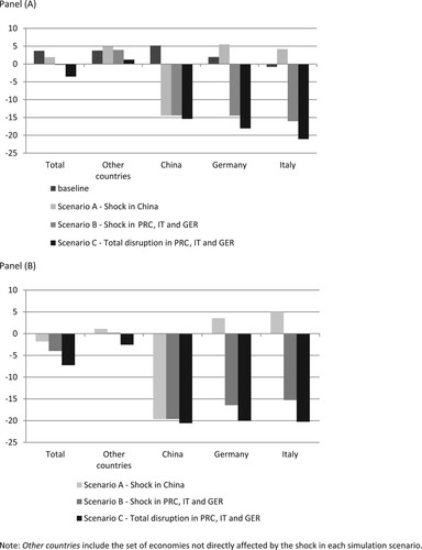
Scenario (B) adds to this initial situation a similar contraction in German and Italian international supply under the assumptions described above. This multicountry shock would not benefit China with respect to Scenario (A) while Germany would move from 2% growth in the baseline scenario to a reduction of about −15% (with an impact, compared to the baseline, of 16.4 percentage points of growth in international trade). A similar effect is observed for Italy. The slowdown in the Chinese, Italian and German exports would result in a zero growth in international trade which would offset the possible benefits for all other producers derived from the absence of the three main competitors in foreign markets. In fact, the rest of the world would remain at the same levels of growth as in the baseline.

Finally, the last simulation includes, in addition to the production freeze in the three exporting countries, a disruption on production chains. Obviously, the implicit hypothesis introduced (no bottlenecks) is valid. In this scenario, the reduction of Chinese, Italian and German production prevents part of the production processes of countries using the intermediates from these commercial areas. This implies damages also for the countries not directly hit by the shock. In fact, the rest of the world would go from a growth of 3.8% of international trade in the baseline to 1.2%. World trade would be heavily affected, with a 3.5% drop in total flows. Therefore the impact on world trade – compared to the baseline in Panel (B) – would be more than 7%. This decrease would not affect all countries equally. There is a reallocation effect of trade flows albeit the total is smaller. It’s important to notice that this effect would be neglected if we had not taken into account the competitive interaction between countries and if we had not endogenously generated the final demand of the different production systems using the national models linked to the trade module.

To further investigate the role of feedback effects, we focus on the results of Scenario (B). Table 1 shows the percentage changes in real total exports due to the partial disruption of Chinese, German and Italian supply chains. The effects are distinguished in direct and direct plus feedback effects. With the first column, we refer to the operating channel of changes in international export flows due to the reduced competition of partially disrupted economies using trade shares estimated with equation 7e. In the second column, total effects include both the change in relative competitiveness on international markets and the reaction to the shock of each country considered in the system. In this case national final demands and domestic prices are endogenously determined through the simultaneous solution of equations 7a–7d and the linkage with the bilateral trade model 7f–7j.

TABLE 1. Total exports (real) – Percentage deviations of Scenario (B) from the baseline.

	Direct effects	Direct + Feedback effects
United States	5.67	2.44
Germany	−12.78	−16.13
Italy	−12.61	−15.39
Japan	5.69	0.61
China	−19.86	−18.66
South Korea	5.93	−1.54

This illustrative example confirms that endogenizing final demand matters. The response to the initial shock in the selected countries presented in the table is heterogeneous. As expected, partially disrupted countries decrease their exports while competitors such as the US, Japan and Korea take advantage of the situation and gain market shares. However, these gains are partially or even completely offset if we consider the feedbacks from national models. On the one side, the increase in import prices for all competitors affects final demand components and decreases personal consumption expenditure and investment both of domestic and imported products. In case the reduction of imports is for intermediate goods, firms will reduce the production of goods using those products as inputs. On the other side, producers might turn to domestic sources of supply, and consumers might change their consumption basket. Those types of adjustments factor in a form of resilience of the national economic systems in response to the international trade disruption.

A further impact of this shock on the welfare of consumers in the national economies can be appraised by the results in Table 2. Here we present the changes in consumption deflators for selected items in United States, Germany and Italy.

TABLE 2. Selected consumption deflators in US, Germany and Italy. Percentage deviations of Scenario (B) from the baseline.

USA
Cereals and bakery products	2.6
Video and audio equipment	2.6
Therapeutic appliances, eyeglasses, contacts	1.9
GERMANY
Beverages	9.9
Food	8.3
Purchase of vehicles	7.5
ITALY
Clothing	4.2
Therapeutic appliances	4.0
Fruit and vegetables	3.8

As personal consumption expenditure is modelled at disaggregate level in our country models,²⁸ we show the results for the three top categories reporting the larger change in deflators in each country. A general increase in the consumption deflators is estimated but the impact is heterogeneous across expenditure categories. For instance, we observe that Germany is mostly affected by the partial disruption of trade flows from China and Italy in food and beverages largely imported from Italy and also in the purchase of vehicles due to imports of parts from Italy and China.

Finally, to further explore the relevance of making national consumption and investment endogenous, we compare the results of Scenario (B) with a simulation that, unlike the previous one, keeps the overall final demand constant, with a similar assumption as used by Dietzenbacher et al. (2019) with the GEM approach. The difference in results between these two simulations will give us a measure of the inaccuracy that one would incur into by neglecting the feedback effects deriving from the endogenization of the different national final demands. Furthermore, it is interesting to verify if these effects are homogenous across commodity groups taking advantage of the multisectoral classification of our international trade module. For convenience of display, four sectors have been selected – Textile fibres, Organic Chemicals, Specialized machinery, General industrial machinery – but similar results can be observed in the whole set of commodity groups included in the BTM. For each sector we have a matrix of origin and destination of the flows, so each cell describes the bilateral relation between a pair of countries for a specific commodity. Every column of this matrix represents a specific destination market and so we know the composition of the exporters to that country. In order to reduce the number of considered flows, we focus our attention only on the bilateral relationships that, compared to the total imports from the destination market, cover at least 5% of the market. Therefore, cells below this threshold are deleted. In Figure 2 the remaining cells are pulled together to represent in a graphical format the total number of trade shares exceeding the threshold in each considered sector.²⁹

FIGURE 2. Impact on bilateral trade relationships of introducing national feedbacks.

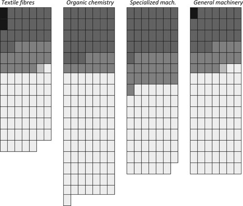
In the four selected sectors, these cells cover 81.1% of the textile fibres market, 77.4% of the organic chemistry, 75.7% of the specialized machinery and 77% of the generalized industrial machinery.

Cells are coloured according to the following criteria. The black cells indicate intersections where the difference between considering feedbacks or not leads to a reversal of the sign of the impact that is particularly marked (a negative impact of more than three points in terms of market share). Dark grey cells are those for which a reversal of the sign of the impact due to the feedback effect occurs but does not exceed the threshold of three percentage points. The grey colour identifies those cells where the sign of the effects of the simulation are confirmed and emphasized once also the feedbacks are considered (without exceeding 3 percentage points). Similarly, cells in light grey are those for which the feedbacks determine a particularly marked accentuation of the simulation results (more than three percentage points). Finally, white cells are those with similar results, with or without feedbacks.

In general, it can be said that in the market of textile fibres about 10.5% of the total trade relations have undergone a reversal of the simulation effects while 48.1% show an accentuation of the simulation results with the final demand constant. Therefore, for almost 60% of the market it is relevant to consider the feedbacks on final demand components and prices. Only 22.5% of international trade in this sector is indifferent to the inclusion of feedbacks. In the organic chemistry market, 26.6% of the relations undergo a reversal of the simulation effects while 15.4% react by accentuating the result already obtained without feedbacks. Therefore 40% of the market is altered in its composition when feedbacks are modelled. In the market of specialized machinery, 23.5% of the trade is affected by the introduction of feedbacks reversing the impact of the simulation and 26.2% instead responds by accentuating the effects of the simulation. Overall, about half of the market is affected by feedbacks. Finally, in the general industrial machinery 22.9% would invert the sign of the simulation effects and 20% would instead increase the effect by keeping the sign.

On the whole, therefore, the endogenization of national final demand components and prices leads sometimes to a striking change of the results, contradicting the simulation results obtained with the hypothesis of keeping the final demand constant.

5. Concluding remarks

The INFORUM international system consists in a Bilateral Trade Model linking a set of country interindustry macroeconometric models (Almon, 2016; Bardazzi & Ghezzi, 2018b). This modelling framework has been widely used for policy simulations and forecasting. In this paper we focused our attention on some properties of this model that are very useful in simulating the consequences of a multinational shock, spreading its effects through the international markets. In our linking system, flows of commodities between countries react to changes in the import-to-domestic-purchase ratios, in the share of bilateral imports and in the level of output of both countries. All these channels are modelled without resorting to fixed proportions or constraining assumptions but through econometric estimation. Moreover, the linkage of national multisectoral models through the bilateral trade model allows to consider the feedback effects on output, prices, employment and final demand components at the country level.

We argue that these characteristics overcome several limitations in the existing literature. On the one hand, the commodity- and country-specific trade shares are endogenous and depend, among other factors, on relative prices. This is a very relevant feature because it allows substitution effects between competitors instead of a pro-rata reallocation of market shares when a shock occurs in an exporting country. Secondly, in our modelling system, it is not necessary to specify any a priori assumption on how the missing – intermediate or final – commodities are replaced. Each national economy adjusts through a change in demand, a substitution with imports from other exporters or with domestic production depending on the relative price competitiveness on domestic and international markets. These adjustments are modelled with the simultaneous solution of the real and nominal sides of the models, taking into account the feedback from trade substitution on IO linkages directly in the dual IO equations which include also the endogenous estimation of several final demand and value-added components. These feedbacks represent a way to factor in country resilience in the simulation of a shock which propagates through internationalmarkets.

Our simulations elucidate some important findings. First, disruption in production of an exporting country has an impact on relative prices in the international markets. This increase in costs affects demand at the country level – including household consumption and investment – and, consequently, total international trade. Moreover, reallocation of market shares is uneven across countries and commodities in both scenarios of a single- and a multi-country shock. The final effect depends on the relative competitiveness on international markets and on the feedback effects from the country models. We have shown that these indirect effects produced from endogenous final demands are significant and heterogeneous across countries. Indeed, in a simulation exercise, we have compared our modelling results with a similar scenario where the final demand at the country level was assumed constant. Our findings for a selection of sectors show that ruling out feedbacks can dramatically change the effects on the bilateral commodity trade flows even reverting the effect of the shock.

To conclude, the characteristics of the INFORUM international system allow us to provide a full picture of the consequences of a disruption in production propagating through the international trade channel. As shown in the empirical examples, the BTM approach not only measures the direct effects but also the feedback effects from the reaction of the national economies. Furthermore, the endogenization of trade shares and value-added and demand components introduces important nonlinearities in the model dynamics with a profound effect on the dimension and on the sign of the shock effects.

Acknowledgements

We like to thank Dr. Douglas S. Meade who has supported this research project since the beginning. We also benefited from the advice and encouragement of Professor Maurizio Grassini from whom we both have learned to appreciate the craft of model building. The usual disclaimers apply.

Disclosure statement

No potential conflict of interest was reported by the author(s).

Additional information

Funding

This work was supported by Jean Monnet Chair HOPPER - Erasmus+ Programme of the European Union: [Grant Number 610775-EPP-1-2019-1-IT-EPPJMO-CHAIR].

Notes

1 Two special issues of Economic Systems Research have been devoted to this theme (n.2, 2007; n.1, 2014).

2 See chapter 3 on IO models at the regional level.

3 Multi-region or world input–output tables are considered as ‘a tool of necessity’ for studying GVC (Antràs & Chor, 2021, p. 4).

4 See Baldwin and Venables (1995) for a critical assessment of CGE models used to evaluate the impact of several regional integration agreements.

5 The claimed parsimony of this approach is limited by the requirement of calibrating all parameters of these models to fit exactly the data including parameters for those pairs of bilateral trade flows taking a value of zero (Antràs & Chor, 2021).

6 This model is an extension of Eaton and Kortum (2002) to a multi-sector economy.

7 As surveyed by Antràs and Chor (2021), the Caliendo and Parro (2015) model has been used for several counterfactual studies on the effects of trade wars, trade agreements and, more recently, the Covid-19 shock (Eppinger et al., 2020).

8 Perfect competition as in Armington (1969), monopolistic competition with homogeneous firms as in Krugman (1980) and monopolistic competition with heterogeneous firms as in Melitz (2003).

9 Structural parameters are either estimated with the dataset used in the analysis (Caliendo & Parro, 2015) or calibrated with elasticities from previous economic literature (see Vandenbussche et al., 2017, 2018, for a recent example).

10 The standard CGE trade model follows the Armington assumption in the trading sector. Under this approach imported commodities are separable from domestically produced goods: firms first decide on the sourcing of their inputs and then, according to the resulting composite import price, determine the optimal mix of imported and domestic goods.

11 For an introduction see Miller and Blair (2009).

12 For a comprehensive overview of HEM-based input–output analyses, see Miller and Lahr (2001).

13 Koks et al. (2019) explicitly tackle this problem by comparing traditional IO models with more recently developed modelling approaches to assess the impacts of supply shocks.

14 In order to analyse also the long run effects, IO techniques are sometimes combined with the CGE approach (Koks & Thissen, 2016) including supply side analysis – to consider potential shortage in inputs –, and substitution effects – to endogenize changes in sectoral output composition.

15 INFORUM (INterindustry FORecasting at the University of Maryland) network was founded by Clopper Almon in 1967 (for a recent account of the main features and evolution of these models see Almon, 2016). The first trade module of the INFORUM international system was built the beginning of the 1970s (Nyhus, 1991). Several developments of the international model followed in later decades as discussed in Bardazzi and Ghezzi (2015).

16 This effect is amplified if the shock is not concentrated just in one country but hits more economies at the same time.

17 For instance, Bardazzi and Grassini (2004) estimate that the indirect effects of the removal of trade and non-trade barriers due to the Eastern EU enlargement are as sizeable as the direct effects.

18 A new dataset of bilateral trade flows has been built with respect to that one described in Bardazzi and Ghezzi (2015, 2018a). This dataset is based on COMTRADE data (United Nations) and collects import flows for all origins and destinations in the world. It covers the period 1995–2017 for all transactions at the two-digit SITC classification level (66 commodity groups).

19 This is defined as a moving average of domestic market prices for the last three years. The price is corrected using exchange rates.

20 The commodity-specific world price is defined as a fixed-weighted average of effective prices in all exporting countries where the trade shares for the base year are assumed to sum to unity to satisfy the homogeneity condition.

21 The world average capital stock is defined as a fixed-weighted average of capital stocks in all exporting countries for a specific sector: $\text{k}{\text{w}}_{\left(\text{y}\right),\text{d},\text{t}}=\sum _{\text{o}}{\text{t}}_{\left(\text{y}\right),\text{o},\text{d},\text{t}=0}\cdot {\text{k}}_{\left(\text{y}\right)\text{o},\text{t}}$, where the fixed weight is t_(i),o,d,t=0

22 This time-trend is cumulated from the complement to 1 of the trade share element, so that as this gets larger the variation of the time variable gets smaller and slows down.

23 Bardazzi and Ghezzi (2018a) present a summary of estimated parameters of BTM: overall, the relative price term is significant in 64% of the trade share equations, while the relative capital stock term in 62%.

24 For a detailed description of the INFORUM approach to multisectoral models, an indispensable reading is the Third Part of The Craft of Economic Modeling (Almon, 2017).

25 Each final demand component may have a detail which is different from the IO classification (e.g. personal consumption is by budget items, investment is by purchasing industries, government expenditure is by budget categories). Bridge matrices are used to convert final demand categories to the IO classification.

26 A third part of the MM (the ‘accountant’) closes the model with respect to income, determines some economic aggregates and estimates transactions which have not been calculated elsewhere in the model. It converts income by sector – divided in several components such as labour income, capital income, and taxes – to the income of various institutions: households, business, government, and the foreign sector. Household disposable income then is used in the consumption functions, while the income of businesses and governments either may be a final variable or may influence investment, interest rates, government expenditures, or other variables. All sides (real, nominal and the accountant) run iteratively until the model converges on a solution.

27 For the sake of simplicity here we put just a vector for final demand but we remind that it is made up of several endogenous components, the most relevant are household consumption expenditures and fixed investments.

28 The classification of expenditure categories is specific for each model according the availability of time-series in each country.

29 Obviously cells are not ordered as in a traditional matrix where the position of the cell inside the matrix explains the origin and destination of the flow.

References

- Almon, C. (1991). The INFORUM approach to interindustry modeling. Economic Systems Research, 3(1), 1–8. https://doi.org/10.1080/09535319100000001
- Almon, C. (2016). Inforum models: Origin, evolution and byways avoided. Studies on Russian Economic Development, 27(2), 119–126. https://doi.org/10.1134/S1075700716020039
- Almon, C. (2017). The craft of economic modeling. Third enlarged edition, www.CreateSpace.com.
- Antràs, P., & Chor, D. (2021). Global value chains. National Bureau of Economic Research, Working Paper 28549.
- Armington, P. S. (1969). A theory of demand for products distinguished by place of production. International Monetary Fund Staff Papers, 16(1), 159–176. https://doi.org/10.2307/3866403
- Baldwin, R. (2016). The great convergence. Harvard University Press.
- Baldwin, R. E., & Venables, A. J. (1995). Regional economic integration. In G. Grossman & K. Rogoff (Eds.), Handbook of international economics, Vol. 3 (pp. 1597–1644). Elsevier.
- Baldwin, R., & Tomiura, E. (2020). Thinking ahead about the trade impact of COVID-19. In R. Baldwin & d. M. B. Weber (Eds.), Economics in the time of COVID-19 (pp. 59–71). CEPR Press.
- Bardazzi, R., & Ghezzi, L. (2015). Towards a new INFORUM bilateral trade model: Data issues and modelling equations. In D. S. Meade (Ed.), In quest of the craft: Economic modeling for the 21st century (pp. 3–42). Firenze University Press. https://media.fupress.com/files/pdf/24/3008/15342.
- Bardazzi, R., & Ghezzi, L. (2018a). Trade, competitiveness and investment: An empirical assessment. Economic Systems Research, 30(4), 497–520. https://doi.org/10.1080/09535314.2018.1446913
- Bardazzi, R., & Ghezzi, L. (2018b). A multi-scale system of macroeconometric models: The inforum approach. Studies on Russian Economic Development, 29(6), 598–606. https://doi.org/10.1134/S1075700718060114
- Bardazzi, R., & Grassini, M. (2004). Measuring the economic impact of the Eastern European enlargement on a EU member state. The case of Italy. In A. Deardorff (Ed.), The past, present and future of the European Union (pp. 159–196). Palgrave MacMillan.
- Barker, K., & Santos, J. R. (2010). A risk-based approach for identifying key economic and infrastructure systems. Risk Analysis: An International Journal, 30(6), 962–974. https://doi.org/10.1111/j.1539-6924.2010.01373.x
- Bekkers, E. (2017). Comparing CGE and NQT models: A formal overview of the model structures. World Trade Organization, mimeo.
- Bems, R., Johnson, R., & Yi, K. M. (2013). The great trade collapse. Annual Review of Economics, 5(1), 375–400. https://doi.org/10.1146/annurev-economics-082912-110201
- Caliendo, L., & Parro, F. (2015). Estimates of the trade and welfare effects of NAFTA. The Review of Economic Studies, 82(1), 1–44. https://doi.org/10.1093/restud/rdu035
- Costinot, A., & Rodríguez-Clare, A. (2014). Trade theory with numbers: Quantifying the consequences of globalization. In G. Gopinath, E. Helpman, & K. Rogoff (Eds.), Handbook of international economics, Vol. 4 (pp. 197–261). Elsevier.
- Dietzenbacher, E., Los, B., Stehrer, R., Timmer, M., & De Vries, G. (2013). The construction of world input–output tables in the WIOD project. Economic Systems Research, 25(1), 71–98. https://doi.org/10.1080/09535314.2012.761180
- Dietzenbacher, E., van Burken, B., & Kondo, Y. (2019). Hypothetical extractions from a global perspective. Economic Systems Research, 31(4), 505–519. https://doi.org/10.1080/09535314.2018.1564135
- Eaton, J., & Kortum, S. (2002). Technology, geography, and trade. Econometrica, 70(5), 1741–1779. https://doi.org/10.1111/1468-0262.00352
- Eppinger, P., Felbermayr, G., Krebs, O., & Kukharskyy, B. (2020). Covid-19 shocking global value chains. CESifo Working Paper 8572.
- Grassini, M. (2013). The core of the multisectoral Inforum model. In R. Bardazzi (Ed.). Economic multisectoral modelling between past and future. Firenze University Press, https://fupress.com/catalogo/economic-multisectoral-modelling-between-past-and-future/2604.
- Haimes, Y. Y., & Jiang, P. (2001). Leontief-based model of risk in complex interconnected infrastructures. Journal of Infrastructure Systems, 7(1), 1–12. https://doi.org/10.1061/(ASCE)1076-0342(2001)7:1(1)
- Hallegatte, S. (2008). An adaptive regional input-output model and its application to the assessment of the economic cost of Katrina. Risk Analysis: An International Journal, 28(3), 779–799. https://doi.org/10.1111/j.1539-6924.2008.01046.x
- Imbs, J., & Mejean, I. (2017). Trade elasticities. Review of International Economics, 25(3), 383–402.
- INFORUM. (1990). Industrial effects of a free trade agreement between Mexico and the USA. A Report for the United States Department of Labor. http://inforumweb.umd.edu/papers/otherstudies/1990/IndustrialEffectsOfUSMexicoFTA_1990.pdf.
- International Monetary Fund. (2020, October). World economic outlook: A long and difficult ascent, Washington D.C.
- Koks, E. E., & Thissen, M. (2016). A multiregional impact assessment model for disaster analysis. Economic Systems Research, 28(4), 429–449. https://doi.org/10.1080/09535314.2016.1232701
- Koks, E., Pant, R., Husby, T., Többen, J., & Oosterhaven, J. (2019). Multiregional disaster impact models: Recent advances and comparison of outcomes. In Y. Okuyama & A. Rose (Eds.), Advances in spatial and economic modeling of disaster impacts (pp. 191–218). Springer.
- Krugman, P. (1980). Scale economies, product differentiation, and the pattern of trade. The American Economic Review, 70(5), 950–959.
- Los, B. (2017). Input–output analysis of international trade. In T. ten Raa (Ed.), Handbook of input–output analysis (pp. 277–328). Edward Elgar Publishing.
- Meade, D. S. (2014). Some thoughts about the interindustry macroeconomic model. Keynote speech at the 22nd International Input-Output Conference, Lisbon, Portugal. http://inforumweb.umd.edu/papers/ioconferences/2014/meade_io2014.pdf.
- Meade, D. S. (2019). Trade war!. [Paper presentation]. 27th International Input-Output Conference, Glasgow, UK. https://www.iioa.org/conferences/27th/papers.html.
- Melitz, M. J. (2003). The impact of trade on intra-industry reallocations and aggregate industry productivity. econometrica, 71(6), 1695–1725. https://doi.org/10.1111/1468-0262.00467
- Miller, R. E., & Blair, P. D. (2009). Input-output analysis: Foundations and extensions. Cambridge University press.
- Miller, R. E., & Lahr, M. L. (2001). A taxonomy of extractions. In M. L. Lahr & R. E. Miller (Eds.), Regional Science perspectives in economic analysis (pp. 407–441). Elsevier Science.
- Nyhus, D. E. (1991). The INFORUM international system. Economic Systems Research, 3(1), 55–64. https://doi.org/10.1080/09535319100000006
- Shelburne, R. C. (2010). The global financial crisis and its impact on trade: The world and the European emerging economies. United Nations Economic Commission for Europe-Discussion Papers Series, 2.
- Timmer, M. P. (2012). The world input-output database (WIOD): Contents, sources and methods. M. P. Timmer (Ed.). WIOD working paper 10. http://www.wiod.org.
- Timmer, M. P., Dietzenbacher, E., Los, B., Stehrer, R., & De Vries, G. J. (2015). An illustrated user guide to the world input–output database: The case of global automotive production. Review of International Economics, 23(3), 575–605. https://doi.org/10.1111/roie.12178
- Tukker, A., & Dietzenbacher, E. (2013). Global multiregional input–output frameworks: An introduction and outlook. Economic Systems Research, 25(1), 1–19. https://doi.org/10.1080/09535314.2012.761179
- Vandenbussche, H., Connell, W., & Simons, W. (2017). Global value chains, trade shocks and jobs; an application to Brexit. Center for Economic Studies Discussion Paper Series, DPS17.13, KU Leuven, September.
- Vandenbussche, H., Connell, W., & Simons, W. (2018). The cost of non-TTIP: A global value chain approach. CEPR Discussion Paper, 12705.
- West, G. R. (1995). Comparison of input–output, input–output+ econometric and computable general equilibrium impact models at the regional level. Economic Systems Research, 7(2), 209–227. https://doi.org/10.1080/09535319500000021