Microdata selection for estimating household consumption-based emissions

Abstract

To estimate household emissions from a consumption-perspective, national accounts are typically disaggregated to a sub-national level using household expenditure data. While limitations around using expenditure data are frequently discussed, differences in emission estimates generated from seemingly comparable expenditure microdata are not well-known. We compare UK neighbourhood greenhouse gas emission estimates derived from three such microdatasets: the Output Area Classification, the Living Costs and Food Survey, and a dataset produced by the credit reference agency TransUnion. Findings indicate moderate similarity between emission estimates from all datasets, even at detailed product and spatial levels; importantly, similarity increases for higher-emission products. Nevertheless, levels of similarity vary by products and geographies, highlighting the impact microdata selection can have on emission estimates. We focus our discussion on how uncertainty from microdata selection can be reduced in other UK and international contexts by selecting data based on the data generation process, the level of disaggregation needed, physical unit availability and research implications.

KEYWORDS:

• Consumption-based footprints
• household consumption
• carbon footprint
• greenhouse gas emissions
• consumer expenditure data
• environmentally extended multiregional input–output analysis

1. Introduction

To meet international and national climate change reduction targets in a socially just manner, it is important for governments to be able to understand and predict greenhouse gas (GHG) emissions and their distributional inequalities. In light of existing research highlighting the need for consumption change beyond technological advances of increased energy efficiency to live within planetary boundaries (Haberl et al., 2020; Parrique et al., 2019; Wiedmann et al., 2020), a consumption-based approach can be a tool to uncover the role of governments in climate change mitigation. While attributing emissions to final consumption should be complementary to other approaches, which focus more heavily on the role of corporate responsibility (e.g. Heede, 2014), supply chains’ impacts on emissions (e.g. Owen et al., 2018), and production-based emissions (e.g. Liang et al., 2018; Sudmant et al., 2018), consumption-based accounting can point to the ways in which policy can target consumption behaviour change (Girod et al., 2014), showcase the effect of infrastructure (Lenzen et al., 2004), and highlight the need to redistribute emissions, energy and resource access to alleviate poverty (Hubacek et al., 2017; see also Spangenberg, 2017).

From a consumption perspective, households make up the end user with the highest emissions – although emissions from other consumption, such as that of governments and investments, should not be overlooked (Hertwich, 2011). To estimate household consumption-based emissions sub-nationally, expenditure and consumption microdata are frequently used. While previous research addresses some limitations emerging from using expenditure as a proxy for volume consumed (Girod & de Haan, 2010), and from inconsitencies between household sruveys and national consumption-based accounts (Min & Rao, 2017), uncertainties around how seemingly comparable microdatasets can impact emission estimates are not yet well-understood. We aim to address this research gap by evaluating the extent to which choice of seemingly comparable consumption microdata can influence emission estimates and make recommendations about how increased robustness can be achieved.

Differential impacts from consumption can be broken down in various ways, such as into consumption patterns, scenarios based on policy recommendations, by socio-deographic groups, and spatially. All of these can be useful in providing different perspectives on carbon inequalities and contribute to understaning how climate change mitigation efforts may be most effective. For example, existing research investigates the carbon emissions of both actual diets and dietary recommendations (Garvey et al., 2021; Hendrie et al., 2014). Similarly, research investigating footprints of people in different income groups highlight the need to not only reduce, but redistribute resources and to target luxury consumption (Büchs & Mattioli, 2021; Millward-Hopkins & Oswald, 2021; Wiedenhofer et al., 2017). Spatially, existing research highlights the importance of place in international (e.g. Ivanova et al., 2017) as well as sub-national (e.g. Clarke-Sather et al., 2011; Jones & Kammen, 2014) contexts. Jones and Kammen (2014), for example, find higher emissions in US suburbs than urban cores and therefore conclude that climate change mitigation efforts need to be place and population specific, underlining the importance of including a donwscaled analysis of space when investigating consumption-based emissions. In line with this, (Lenzen et al., 2006) point to differences between countries, not just in energy needs, but also in social drivers of energy needs. These can vary drastically due to countries’ unique situations regarding factors such as climate, history, culture, and existing infrastructure, highlighting that place-specific understandings of energy need and carbon emissions are vital for reducing emissions. Moreover, UK-based research finds stark inner-city differences in London (Minx et al., 2013; Owen, 2021). However, as that research is at a local governmental area, or Local Authority District (LAD), level, inner-city differences outside of London and localised details of footprints cannot be investigated. Consequently, to enable a detailed understanding of spatial carbon inequality, a sub-district analysis is needed. In addition, a product-level disaggregation allows for a greater understanding of the context in which spatially specific patterns of consumption occur. For instance, Australian research suggests that higher income neighbourhoods may have better access to public transport links, reducing private transport emissions and thus emphasising the impact of local infrastructure and access to services on consumption-based emissions (Lenzen et al., 2004). Local, product-level consumption-based emissions can aid local strategies, by providing a spatial overview of sub-national carbon and energy inequalities, and a point for analysis of local and national governmental mitigation efforts. Such efforts might include local transport and infrastrucutre planning, localised behavious change campaigns, or housing startegies. Indeed, recent years have seen an increased involvement of local actors in tackling climate change, including global (e.g. C40 Cities, 2020) and local city-level initiatives (DEAL et al., 2020). In the UK, local governments are increasingly making declarations of climate emergencies (LGA, n.d.), with London Councils targeting a reduction in emissions of two thirds by 2030 (Gilby, 2021), and cities like London and Bristol have begun tracking neighbourhood footprint trajectories (Owen, 2021; Owen & Barrett, 2020a; Owen & Kilian, 2020).

To investigate consumption-based emissions sub-nationally, microdata on consumption are needed to disaggregate national accounts. As microdata are not available for every neighbourhood, however, data modelling and different data generation processes increase uncertainty in emission estimates. Using the UK’s 2016 consumption-based emissions as a case study, we explore how differences in microdata can shape neighbourhood emission estimates and make recommendations about which factors to consider when selecting microdata. The UK makes for a compelling case study for various reasons, most importantly it is a net-importer of GHG emissions (Defra, 2020). In addition, the UK reports annual consumption-based emissions accounts as a National Statistic (Defra, 2020) and has a national framework to measure consumption-based emissions (the UK Multiregional Input–Output Model (UKMRIO)), as well as a variety of public and private microdatasets which allow for a detailed breakdown of national emissions. Whilst data availability and access arrangements vary globally, the UK example highlights how the use of different microdata could result in different policy conclusions and reveals where additional care should be taken when selecting microdata.

While uncertainties across different expenditure microdata are under-explored in the consumption-based accounting literature, methodological limitations, as well as uncertainties from input–output data are well-documented. Different input–output databases can vary drastically with regards to sector aggregation, availability of time series data, and inclusion of uncertainty estimates (Hoekstra, 2010; Owen, 2017; Tukker & Dietzenbacher, 2013), causing them to have different strengths and weaknesses. Moreover, consumption-based inventories carry higher levels of uncertainty than production-based accounts, as these are in closer proximity to statistical sources (Peters, 2008). Lenzen et al. (2004) summarise the sources of these as erroneous sampling, sector aggregation, limiting products’ lifecycles from production to consumer, and assumptions around factor multipliers between domestic and competing foreign industries being the same, foreign industry homogeneity, and monetary flow being a good proxy for physical flow. To quantify the uncertainties, studies have investigated both source and multi-regional input–output (MRIO) data. Uncertainties of MRIO databases are estimated to be higher at sectoral than at national level (Karstensen et al., 2015; Rodrigues et al., 2018). Additionally, these can vary by territory, with uncertainties ranging from 5% to 10% in OECD and from 10% to 20% in non-OECD countries, at country level (Rodrigues et al., 2018), and uncertainties being lower in larger regions, such as the European Union (Wood et al., 2019). Despite differences in estimates, Moran and Wood (2014) find that patterns of change over time are comparable between global MRIO models. Thus, while differences in industry carbon emissions data may lead to variations in results, trends in outputs are comparable across the databases. Using a single-country National Accounts consistent footprint, where an existing global MRIO database is adjusted to national data on environmental footprints, may increase robustness (Tukker et al., 2018). The UKMRIO used in the current research uses this methodology outlined by Tukker et al. (2018) to reduce uncertainty. Finally, research on the UKMRIO, though dated, suggests that the UKMRIO is a robust framework for assessing consumption-based emissions, with higher uncertainties at sectorial level (Lenzen et al., 2010; Wiedmann et al., 2008).

A second area of uncertainty is related to splitting national into sub-national emissions. Sub-national estimates of environmental pressure data can be estimated in different ways when using Input–Output models, including with consumption and expenditure data and spatially-specific MRIO databases (see Ploszaj et al., 2015; Sun et al., 2019). Here we focus on those sub-national emission estimates generated with household expenditure data, as these are often the most accessible and a frequently used way of disaggregating national accounts (e.g. Minx et al., 2013; Pothen & Tovar Reaños, 2018; Steen-Olsen et al., 2016). Here, various limitations arise. Firstly, error is introduced due to inconsistencies between household surveys and national accounts as well as aggregation of different sectors when matching national accounts with household surveys. Min and Rao (2017) estimate this error to be at around 20% for India and Brazil. Secondly, disaggregating national consumption-based accounts using spend data can be problematic where the same products vary in price. For example, cheap supermarket bread does not necessarily have lower consumption-based emissions than an expensive artisan loaf. To reduce this uncertainty, some research uses other measures of consumption. For instance, existing research from Australia (Hendrie et al., 2014) and the US (Goldstein et al., 2017) uses physical data from nutrition surveys to estimate food emissions. Data on other consumption measures, such as on household energy consumption (e.g. EIA, n.d.; UK: BEIS, 2020a, 2020b) and transport (see Jones & Kammen, 2014) are also available in some countries, although not all can be disaggregated spatially. Despite this, depending on the country and context, even research which replaces some expenditure data with physical measurements, such as weight, (e.g. Vita et al., 2019) often relies heavily on expenditure data, due to the unavailability of other measures of consumption. Girod and de Haan (2010) estimate that approximately 50% of increased spending of high-income Swiss household can be linked to higher purchase prices, while the other 50% is linked to increased consumption. However, while this may lead to an underestimation of low footprints and an overestimation of high footprints, overall trends remain measurable. Nonetheless, despite this additional uncertainty, lack of data availability often does not allow for functional unit use. In addition to these commonly reported uncertainties, this research aims to assess to what extent choice of seemingly comparable consumption microdata can influence emission estimates and to make recommendations about how increased robustness can be achieved.

To review microdata differences, we compare household GHG emission estimates generated from three UK household expenditure datasets, at a product and neighbourhood level following data validation guidelines from Eurostat (Zio et al., 2016). Two of the datasets we compare are considered open data, one of which is publicly available. With most nations having a 2020 census cycle (UN: Statistics Division, 2021) – including the upcoming publication of new UK census data in 2021 –, an increased interest of local government bodies to track sub-Local Authority emissions (Owen & Barrett, 2020a; Owen & Kilian, 2020), increased use of open data, and city-government calls for climate emergencies, it is important to validate emissions generated using different microdata, and to assess their usefulness for different purposes. We provide an overview of the robustness of product-level consumption-based emissions at a neighbourhood level, to give recommendations about various levels of product and spatial-aggregation which can also be employeed outside of the UK context, and to provide an openly available method for local governments to track emissions over time.

Finally, in order to facilitate an accessible and replicable method which can be reproduced by local governmental bodies, a move to open data is beneficial. Despite growing demands for increased reproducibility across the social sciences (Brunsdon, 2016; Tay et al., 2016), consumer data is often commercially created, resulting in much research on consumption-based emissions using commercial expenditure datasets (e.g. Baiocchi et al., 2010; Minx et al., 2013). Not only does this mean that data are less accessible to other researchers and policy makers by being behind a pay-wall, but also that data generation processes are often not fully transparent. In line with arguments presented by Pfenninger et al. (2017) we include two openly available datasets within this research. Although open data are not strictly necessary for this type of research, they can provide more transparency and a more replicable method.

In the following section we describe the methods used to both generate the various neighbourhood and product-level emission estimates as well as how we assess their similarity. This is followed by our findings, and a discussion of the findings, in which make internationally-applicable recommendations about microdata selection based on the data generation process, the level of disaggregation needed, physical unit availability and research implications.

2. Materials and method

2.1. Data and access

This research uses a combination of geographic data, census data, expenditure data, and input–output data to estimate consumption-based neighbourhood emissions using three seeminlgy comparable household expenditure microdatasets. These estimates are then analysed to assess how different microdata influence emission estimates.

2.2. Neighbourhood-level household expenditure microdata

The expenditure microdatasets used to disaggregate UK national emission estimates to a neighbourhood level are the Living Costs and Food Survey (LCFS), Output Area Classification (OAC), and a rarely used commercial consumer expenditure dataset by TransUnion. Expenditure from all datasets is from the year 2016, using 2016 prices, as it is the most recent year for which all three datasets are available.

The LCFS is an openly available annual expenditure survey recording detailed spends from 4000 to 6000 private households across the UK (ONS, 2017b). Expenditure is recorded for two weeks for everyday items and for up to 12 months for infrequently purchased items. To ensure representativeness, the LCFS uses a multi-stage stratified sample in Great Britain and a systematic random sample in Northern Ireland (ONS, 2017b). Moreover, the LCFS has quotas for household types and geographic areas to ensure a nationally representative sample (ONS, 2017b). The LCFS used in the current analysis is from the year 2016/17 and can be accessed through the UK Data Service (ONS & Defra, 2020). In 2016/17, 5041 households were surveyed. In addition to expenditure, the LCFS contains physical units for certain products, such as number of flights taken.

Expenditure in the OAC and TransUnion is modelled from the LCFS, highlighting the central role the LCFS plays in measuring household expenditure in the UK. Many other UK household expenditure datasets, including publicly available household expenditure datasets (e.g. ONS, 2020a), are derived from the LCFS, as it is a comprehensive, annual national statistic. As a result, this research compares a variety of end-products derived from the LCFS, which, despite similarities in the primary data generation process, have varying strengths and limitations as a result of secondary modelling differences.

The OAC is the UK’s publicly available geo-demographic classification, whose current version is created from 2011 census data (Gale et al., 2016). It clusters Output Areas (OAs), the smallest census area geography, by socio-demographic similarities and thus represents a summary of multivariate categories. Classifications incorporate information from 60 census variables, including ones on age, ethnicity, dwelling type, and employment (Gale, 2014; Gale et al., 2016). Each OA is thereafter assigned a classification. The OAC is available at 3 different levels: supergroup (8 classifications), group (26 classifications), and subgroup (76 classification).¹ Here the ‘group’ level is chosen, as this provides a good balance of product and spatial detail.² Supergroups include classifications such as ‘suburbanities’, which is made up of the two group level classifications ‘suburban achievers’ and ‘semi-detached suburbia’. Classifications for all supergroup, group, and subgroup levels can be found in (Gale et al., 2016). OAC expenditure profiles are updated every 2–3 years based on expenditure from the LCFS, with the one used in the current research being for the years 2015–2017; the classification process occurs only every 10 years.

Lastly, the TransUnion dataset, while based on the LCFS, considers the mix of housing types in each OA for its estimates of consumer spending. This makes the TransUnion dataset more spatially-detailed than the OAC, and our regional LCFS expenditure profiles. While this dataset does not have a fully transparent modelling process, due to its commercial nature, the spatial detail and rare access to these data in academic research make this dataset a valuable and novel resource for this research. The three expenditure datasets are chosen for their respective strengths and limitations (Table 1), which can provide a thorough comparison of their respective emissions estimates, as well as data availability. All datasets contain all households spends and follow the structure of Classification of Individual Consumption by Purpose (COICOP) (UN: Statistics Division, 2019), which means that the expenditure categories from all datasets are complete and map onto each other.³ The OAC and TransUnion data are structured by COICOP 3 categories, which include detailed spends such as ‘Milk’, ‘Bus and Coach Fares’, and ‘Women’s Outdoor Apparel’. The LCFS also contains expenditure at a more detailed COICOP 4 level for many products and services.

TABLE 1. Strengths and limitations summarised.

**Notes: Robustness to Outliers cannot be determined for TransUnion as the exact modelling process is unknown. OAC product detail is high at group and supergroup levels.

The LCFS is the most comprehensive consumption and expenditure survey in the UK and thus sets the basis for much expenditure microdata available. Despite the three datasets all being derived from the LCFS being a potential limitation in this study, the three datasets are fundamentally different in the way they are modelled to represent the whole UK, rather than just the survey participants. The OAC assigns expenditure based on demographic similarity, the TransUnion dataset is a commercial product which uses localised information on household types, and while the LCFS modelling we did here relies on the OAC it also includes geographic information from regions and thus disaggregates expenditure in a way that incorporates more spatial detail than the OAC does. These differences allow us to see how the different modelling processes impact our emission estimates. Indeed, being derived from the same base product may make differences more striking and provide insight into how the modelling processes can shape emission estimates.

2.3. Multiregional input–output data

To calculate the GHG emissions associated with the consumption-patterns of UK neighbourhoods we need a set of product-based conversion factors that can be used to convert household activity into emissions. Conversion factors need to take into account both the direct emissions associated with burning fuel to heat homes and drive cars and the indirect emissions associated with the full production supply-chain of the goods and services bought by the household. In addition, the factors should include both emissions from domestic production and those emissions released abroad which are used in the production of imports.

MRIO databases have been used by environmental economists due to their ability to make the link between the environmental impacts associated with production techniques and the consumers of products. The Leontief input–output model is constructed from observed economic data and shows the interrelationships between industries that consume goods (inputs) from other industries in the process of making their own products (outputs) (Miller & Blair, 2009). The fundamental Leontief equation, x = (I − A)⁻¹y, indicates the inter-industry requirements of each sector to deliver a unit of output (x) to final demand (y).⁴ Since the 1960s, the input–output framework has been extended to account for increases in the pollution associated with industrial production due to a change in final demand. Consider, F = eLy where F is the GHG emissions in matrix form. F is calculated by pre-multiplying L by e, emissions per unit of output, and post-multiplying by final demand y. The vector eL is a product-based full-supply chain conversion factor for indirect emissions. In addition to inter-industry requirements, an MRIO framework is also able to account for imported goods and differences in emission intensities which occur throughout the supply-chain arcoss different regions.

We use the UKMRIO to calculate the conversion factors for the year 2016 at current prices: GHG per unit spend (£) by COICOP product (Defra, 2020; ONS, 2019, 2020b). The UKMRIO is a national statistic constructed annually by the University of Leeds following methodology outlined by Tukker et al. (2018) and Edens et al. (2015). Greenhouse gases reported in the UKMRIO are carbon dioxide (CO₂), methane (CH₄), nitrous oxide (N₂O), hydrofluorocarbons (HFCs), perfluorocarbons (PFCs), sulphur hexafluoride (SF₆) and nitrogen trifluoride (NF₃), these are converted into their carbon equivalent and are reported as tCO₂e. A more detailed description of the UKMRIO can be found in Owen and Barrett (2020b). A unique feature of the UK Supply and Use Tables used to construct the UKMRIO is the diaggregation of the column of household final demand into COICOP categories providing a COICOP to SIC bridging table. Thus it is straightforward to calculate the GHG emissions associated with household spend by COICOP product. After direct emissions from burning fuel to heat homes and drive cars are added to the relevent COICOP products,⁵ emissions by COICOP can be divided by total household spends reported in the LCFS to produce a COICOP product-based full-supply chain conversion factor for both direct and indirect emissions.

2.3.1. Geographic, census, and other data

Geographic and census data used in this research are all publicly available. To estimate neighbourhood emissions, we use data from the 2011 census for OA populations, geography lookup tables, and geographical boundaries (National Records of Scotland, 2013; NISRA, 2013; ONS, 2013), and from the ONS (2017a) for the 2016 mid-year populations. In addition, as physical use proxy data (see section 3.3) we use levels of car ownership from the 2011 census, and gas and electricity consumption data from the Department for Business, Energy and Industrial Strategy (UK: BEIS, 2020b, 2020a).

This research aggregates emissions to small neighbourhoods (Lower Super Output Area (LSOA)) and medium neighbourhoods (Middle Super Output Area (MSOA)), the second and third smallest census geographies in England and Wales, respectively. Geographies vary slightly by the different countries in the UK. Equivalents from Northern Ireland and Scotland are chosen based on area populations. For easier reading, this paper refers to the English and Welsh names (OA, LSOA and MSOA), even where equivalents from Scotland and Northern Ireland are used. A summary of these is provided in Table 2, with more details provided in Appendix A.

TABLE 2. Summary of UK neighbourhood geographies used in this research.

	Description and demographics		Naming throughout the UK
	Population	Number of Units in the UK	England and Wales	Scotland	Northern Ireland
Smallest Census Geography	50–700	232,296	Output Area	Output Area	Small Area
Small Neighbourhood	500–3000	42,619	Lower Super Output Area	Data Zone	Super Output Area
Medium Neighbourhood	2000–15,000	9062	Middle Super Output Area	Intermediate Geography	Ward^a

^a A ward is a geographic area at a more aggregated scale than an MSOA level. Wards mainly reflect electoral wards (ONS, n.d.). This is chosen as it is the Northern Irish geography most like MSOAs by population.

2.3.2. Data pre-processing

Product-level expenditures from the expenditure microdatasets are adjusted to household final demand figures reported in the UKMRIO, to ensure that all expenditure reported in the UKMRIO is accounted for. Secondly, using a physical measure of accommodation, such as number of rooms may be better than a financial measure, as rents can vary drastically by region, even when housing size is controlled for (ONS, 2020c; von Auer, 2012). Therefore, number of rooms is used as a physical proxy for both the LCFS and OAC, the two datasets containing this measure. In addition, the LCFS allows for the adjustment of expenditure data on flights through physical units, as information on the number of domestic and international flights taken is provided.⁶

Moreover, households paying by direct debit or monthly instalments pay approximately 80 GBP less per year for gas and electricity, due to using different payment methods (OFGEM, 2014). Payment type is also often linked to income and house ownership, with low-income households and renters being more likely to have pre-paid utilities. As payment method information is available for gas and electricity consumption in the LCFS and can be matched to the OAC through the census (National Records of Scotland, 2013; NISRA, 2013; ONS, 2013), expenditure for electricity and gas use is adjusted for the OAC and LCFS.

Spatially, the LCFS includes information on regions⁷ and OAC. To disaggregate beyond regional level, we group weekly expenditure data from the LCFS by OAC and regional information. This allows us to create regional expenditure profiles, which we can associate with specific geographic location, whereas the OAC expenditure profiles relate only to OAC group, but not spatial location. This is done using all three levels of the OAC, such that the highest level of disaggregation is possible, while ensuring that each grouping contains a minimum of 10 observations; this provides groups small enough to attain high spatial detail, while being large enough to maintain a mean that in most cases is not dominated by one observation. Moreover, later aggregation to higher geographies further increases group sizes and thereby helps further reduce susceptibility to outliers. More details can be found in Appendix B.

Aggregation to a minimum of 10 surveys results in 283 expenditure groups with regional information. Of the 5041 surveys, 9 could not be grouped due to missing OAC values. A further 237 could not be included in the regional profiles because no group with more than 10 observations could be made below national level. These are mainly for OACs not common in a region, and as OAs are aggregated to higher geographies after footprint calculation, results will not be significantly affected by this. Separately, footprints are also calculated based only on a LCFS-aggregation by OAC supergroups, which are attached to OAs in instances where the UK’s OAs do not match any of the region-specific profiles generated.

Population estimates attached to each expenditure dataset are adjusted to the 2016 mid-year population estimates, such that proportions of populations within a certain expenditure category are kept the same as they are in the expenditure datasets, but the total population is adjusted to the mid-year estimates. This controls for slight population differences between the datasets and allows for better comparison of emission estimates.

2.4. Analysis

An environmentally-extended input–output analysis is employed to estimate household GHG emissions using all three household expenditure datasets. Neighbourhood GHG emissions are calculated using the highest product and service level available for each survey. Thereafter, findings are aggregated to LSOA and MSOA levels and compared at COICOP 2 and COICOP 3 levels. To prevent a spurious correlations by using multiple variables which are derived from common ancestors (Pearson, 1897; Ward, 2013), per capita tCO₂e rather than total population emission estimates are used for each MSOA and LSOA in our analysis.

To validate our emission estimates we follow guidelines from the Eurostat ESSnet ValiDat Foundation (Zio et al., 2016). As these guidelines also include error location for big data analysis, we follow only the validation levels applicable to the current research. These include checking for consistency within the dataset, consistency to other similar datasets (which is the main aspect of this paper), and, where possible, we compare our emission estimates to physical use data or proxies from other data providers.

To compare various aspects of the data we use multiple statistical comparisons. As data are non-normally distributed we employ a Friedman test⁸ to assess whether the results from the three datasets are statistically derived from different distributions (Friedman, 1937). In addition, to assess covariance we run a Spearman’s ρ correlation analysis. As large sample sizes can inflate statistical significance testing, we focus on effect size for both tests. As is common in statistical analysis, we interpret effect size from the Friedman test (Kendall’s W value) to be small if it is below 0.3, and the correlation coefficient to indicate at least a weak correlation if it is 0.3 or above. Both tests assign ranks and as a result can only be used to understand distributions and covariances, but not magnitudes of similarities and differences. To understand dataset differences and similarities between actual emission values we therefore also calculate and compare the root mean squared errors (RMSEs) of the three dataset comparisons. RMSEs are in the unit of measurement and thus need to be interpreted in relation to emission estimates.

3. Results

3.1. Total per capita consumption emissions of UK neighbourhoods

The mean household consumption emissions for the UK are 9.36 tCO₂e per capita for the year 2016. At both MSOA and LSOA levels, 80% of total per capita emissions range from 7 to 12 tCO₂e, in all three disaggregation methods. While distributions of emissions from the LCFS and TransUnion datasets are similar with one peak, the OAC results have a multimodal distribution at neighbourhood levels (Figure 1).

FIGURE 1. Distributions of per capita footprints of UK LSOAs and MSOAs. Vertical lines show the 25th, 50th, and 75th percentiles.

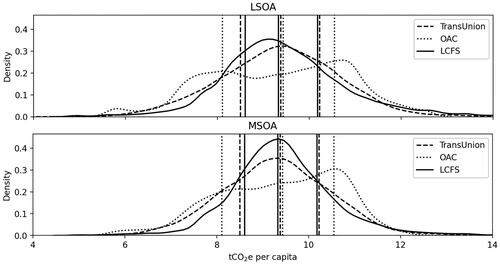
This is stronger at LSOA than at MSOA level, likely pointing towards the limited number of categorised expenditure profiles in the OAC, as well as to some profiles being much more common than others; for instance, groups falling within the ‘Suburbanites’ and ‘Hard-pressed living’ supergroups make up approximately 40% of OAs.

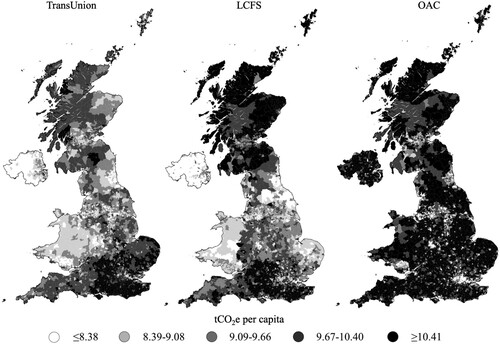
Some differences are also evident spatially. The spatial distributions of MSOA per capita GHG emissions are shown in Figure 2. The OAC footprints are high in rural areas without much variance as only 3 of the 26 profiles are linked to rural areas, whereas the TransUnion and LCFS emissions appear to have more nuanced variances over space. The OAC may therefore be less precise in rural than in urban areas. Moreover, the OAC results do not show possible regional differences, as the OAC is a UK-wide classification, regional variances may therefore get overlooked. These include possible lower emissions in Northern Ireland and Wales, which we find with the other two datasets. Finally, the LCFS assigns rural parts of Scotland higher emissions than the other two datasets, however, as populations are small, footprints for the total population in Scotland are among the lowest in the UK.

FIGURE 2. UK MSOA per capita GHG emission quintiles.

A statistical comparison of the datasets is undertaken, where distributions, correlation coefficients and RMSEs are analysed. A Friedman test finds negligible effect sizes of Kendall’s W = 0.01 for both MSOAs and LSOAs, indicating that the difference between distributions is only very weak. Similarly, at both geographic levels data have Spearman’s ρ correlation coefficients of 0.44 or stronger, indicating at least moderately strong correlations between emission estimates from all datasets (see Table 3). RMSE results show mean errors of 10–17% of the UK mean per capita emissions. Emission estimates from TransUnion and the LCFS appear to be most strongly correlated and have the lowest error. This is reflective of the higher levels of spatial detail in the LCFS and TransUnion datasets and indicates that the LCFS may a better open data option than the OAC at disaggregating total emissions spatially, to a neighbourhood level.

TABLE 3. Statistical results for total emissions.

		Spearman’s ρ			RMSE
Geography	Kendall’s W (Friedman test)	OAC & TransUnion	OAC & LCFS	TransUnion & LCFS	OAC & TransUnion	OAC & LCFS	TransUnion & LCFS
MSOA	0.01	0.47	0.44	0.62	1.29	1.34	0.95
LSOA	0.01	0.53	0.46	0.53	1.39	1.56	1.25

3.2. Product-level findings

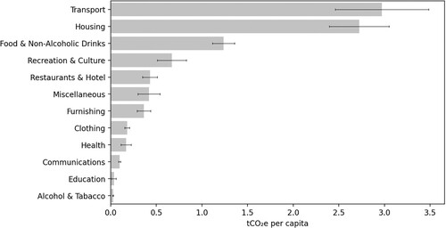
In the UK, household consumption-based emissions are highest for emissions related to transport, followed by housing and food and drinks (see Figure 3). These product and service categories can be further disaggregated, such as into COICOP 2 and COICOP 3 product and service categories. This section focuses on UK neighbourhood emission estimates produced by the three microdatasets for these more disaggregated product and service. A full list of COICOP 1, 2, and 3 categories can be found in Appendix C.

FIGURE 3. Mean UK per capita GHG emissions by COICOP 1 categories from all datasets.

**Notes: Error bars show the standard deviation from MSOA-level results across all three datasets.

Distributions, covariance, and error are also analysed at COICOP 2 and 3 product/service levels. We consider a product/service category to ‘pass’ the Friedman validation test if it has Kendall’s W < 0.3 and to ‘pass’ the correlation validation test if it has Spearman’s ρ ≥ 0.3. As shown in Table 4, we find that product/service categories that pass all tests only make up around half of the UK consumption-based household footprint. For most geographic and product levels rates for number of products are a little lower, suggesting that higher-emitting products and services more often have more similar distributions and higher covariance than lower-emitting ones. Notably, results from individual tests are higher than those considering all tests. This shows that differences between the datasets occur down to a product level, or in other words, that dataset differences are not consistent across product/service categories. Moreover, correlation results from the LCFS and TransUnion comparison are lower than those from other comparisons, contradicting the total emission comparisons and hinting at the impact different microdata generation processes can have on product-level emission estimates. Finally, higher level aggregation almost always increases total pass rates, showing convergence to the mean with decreased detail. Exempt from this are COICOP 2 level difference between MSOA and LSOA; here it may be that aggregation to an MSOA level merged LSOAs with high levels of dataset similarity with LSOAs with low levels of similarities between datasets. These exceptions are likely data-specific and dependent on individual outliers rather than systematic emission estimate generation processes.

TABLE 4. Percentages of total tCO₂e / capita from products and number of products passing the Friedman (Kendall’s W < 0.3) and correlation (Spearman’s ρ ≥ 0.3) validation tests.

		Total tCO2e / capita (%)					Number of products (%)
				Passed correlation test					Passed correlation test
COI-COP	Geo-graphy	Passed all tests	Passed Friedman test	LCFS & TU	OAC & LCFS	OAC & TU	Passed all tests	Passed Friedman test	LCFS & TU	OAC & LCFS	OAC & TU
2	MSOA	51.98	100.00	53.30	68.82	60.17	56.41	100.0	64.10	74.36	82.05
	LSOA	63.30	100.00	64.50	66.88	73.48	53.85	100.0	58.97	66.67	87.18
3	MSOA	51.10	85.17	66.74	78.31	74.25	44.78	90.30	55.97	79.10	68.66
	LSOA	46.08	85.42	60.68	75.32	74.59	38.81	91.04	46.27	70.90	68.66

**Notes: The UK has a footprint of 9.36 tCO2e / capita. The COICOP 2 classification contains 39 product and service categories, the COICOP 3 classification contains 134 product and service categories.

Results for individual product/service categories are shown in Figure 4. This highlights various important characteristics of the results. Firstly, there is significant overlap in the distribution and covariance tests between LSOAs and MSOAs at both product levels, indicating that dataset differences are more consistent across geographic disaggregation than product-level disaggregation. Secondly, most product/service categories which did not pass all tests, failed more than one test. This suggests that some products may be more dissimilar than others and that by using physical data for such products uncertainty may be reduced. Thirdly, per capita footprints are logarithmically distributed between products, with only very few product and service categories having high per capita emissions. This indicates that there are a few products and services for which estimating accurate emissions is more important. Indeed, the product and service categories with the highest per capita footprints (COICOP 2: ‘Electricity, gas and other fuels’; COICOP 3: ‘Gas (Home)’) failed all correlation tests across both geographies. Given that gas pricing in the UK can vary according to payment type and time of day this finding is not surprising and emphasises the need for a physical unit measure rather than expenditure to disaggregate household gas emissions sub-nationally. Interestingly, however, ‘Electricity (Home)’ alone, passes all tests, indicating that microdata are more similar for electricity than for gas expenditure. While this does not indicate that a physical unit measure may not be better, it does show that monetary data from the three microdatasets disaggregated the footprints similarly across neighbourhoods.

FIGURE 4. Detailed selected results from Friedman test and correlations (black cells indicate a failed test), and mean emissions and RMSEs. Results are displayed for highest-emitting products contributing to over 80% of consumption-based emissions; this constitutes 23% of COICOP 2 and 21% of COICOP 3 products/services.

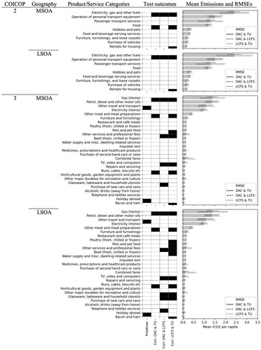
Finally, despite having a small RMSE between all three datasets pairings, ‘food’ and ‘other meat and meat preparations’ – the highest food-related COICOP 3 category – fail the correlations tests involving the TransUnion data in most product- and neighbourhood-level combinations. This indicates that the OAC and LCFS report more similar food expenditure than the TransUnion data. Although we cannot be certain why the TransUnion data are different, as their data generation process is not fully available, it is possible that this difference is due to the LCFS and OAC establishing mean expenditure over regions and the whole UK. It may be, therefore, that price differences from purchasing different kinds of food products that fall within the same COICOP category have a higher convergence to the mean for the LCFS and OAC. Reversely, price differences may impact emissions more strongly when using the TransUnion data to disaggregate national accounts.

Moreover, knowledge about the various data generation and modelling processes may further inform why differences occur and which dataset may be most suitable for which type of analysis. Finally, RMSEs are mainly proportional to mean emissions and comparable across dataset pairings. Again, products linked to home gas use have disproportionally high errors, mirroring findings from the correlation analysis. Notably, errors are also higher for pairings including the LCFS for the COICOP 2 category ‘Passenger transport services’. This category includes emissions from flights, which are likely more accurate for the LCFS than the other two datasets, as number of flights was used to disaggregate emissions instead of flight expenditure.

3.3. Physical proxy-data comparisons

To evaluate which dataset best represents physical units, we also compare the different emission estimates to physical use proxies. We use simple linear regression models to assess which estimates can best predict physical use proxies. Physical use proxy data are available for three high-emission COICOP 3 categories at a neighbourhood level in the UK: ‘Electricity’, ‘Gas’, and ‘Petrol, diesel and motoring oils’. For gas and electricity we use consumption data available via BEIS (UK: BEIS, 2020b, 2020a), which is available for England, Wales, and Scotland at both MSOA and LSOA levels for 2016. As a proxy for proxy for ‘Petrol, diesel and motoring oils’, we use 2011 statistics of amount of car ownership⁹ from the census, which are available for the whole UK. Model validation is done by splitting the data into an 80% train and a 20% test set and indicates no concern of overfitting.

Results indicate that the OAC and LCFS can best predict ‘Electricity’ and ‘Gas’ use respectively, although fits for all models are poor (Table 5). RMSEs are at around 18-26% of mean values for both gas and electricity, but at a lower 7-15% for car ownership. Levels of car ownership are also better predicted by our emission estimates, with good model fits for the OAC data, and moderate model fits from the LCFS. The TransUnion data performs poorly on all variable predictions. It should be noted that high levels of car ownership do not per se mean that emissions should be higher, as car use emissions can be linked to other factors such as infrastructure, place, and public transport links. Despite this, lower car ownership levels should also come with decreased emissions. Thus, while high levels car ownership may not be a good proxy for emissions, we expect low levels of car ownership to be paired with low emissions. As shown in Figure 5, both the LCFS and the OAC show low emissions from car use, in neighbourhoods with low car ownership. The TransUnion data, on the other hand, assigns similar levels of emissions from motoring oils across neighbourhoods with different levels of car ownership. As census variables, including car ownership, are used to generate the OAC expenditure profiles, the OAC may best capture distributions of emissions related to these variables. This is followed by the LCFS as used here, where OAC data are incorporated to model expenditure across the UK.

FIGURE 5. Scatterplots showing levels of car ownership vs emissions from ‘Petrol, diesel and motoring oils’.

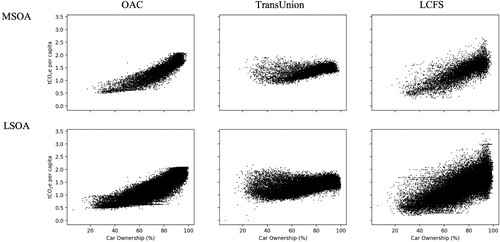
TABLE 5. Prediction model summaries.

		MSOA				LSOA
Product/Service	Dataset	AIC	RMSE	R^2 (train)	R^2 (test)	AIC	RMSE	R^2 (train)	R^2 (test)
Electricity	OAC	107,328	683.35	0.19	0.19	542,315	806.31	0.13	0.14
	TransUnion	108,610	755.34	0.02	0.01	546,726	866.01	0.01	0.01
	LCFS	108,708	759.98	0.00	0.00	546,943	868.68	0.00	0.00
Gas	OAC	124,561	2643.57	0.08	0.09	628,035	3304.35	0.05	0.11
	TransUnion	125,092	2758.14	0.01	0.01	629,552	3470.67	0.01	0.01
	LCFS	123,146	2374.76	0.26	0.27	624,500	3054.26	0.15	0.24
Petrol, diesel and motoring oils	OAC	47,226	7.16	0.79	0.77	239,853	8.29	0.74	0.75
	TransUnion	56,114	13.16	0.25	0.24	274,922	14.12	0.27	0.26
	LCFS	51,630	9.97	0.60	0.56	264,566	11.92	0.46	0.47

** Notes: R² model fit is shown for both the training (80% of dataset randomly selected) and testing sets (20% of dataset randomly selected). The best model fits for each product/service are highlighted in boldface. Mean values are around 3800 kWh for electricity and 13,500 kWh for gas, for reference for RMSE interpretation.

3.4. Local Authority District level analysis

For policy purposes it is important to understand the dataset variance at an LAD level, whose boundaries are defined by local government districts, as this is where policy decisions can be made. An analysis of LSOA and MSOA footprints is therefore done within LAD boundaries to assess the similarity of neighbourhood emission within a local administrative boundary. Hence, instead of correlating product and neighbourhood emission estimates from the three datasets at a national level, as done in the previous section, here we correlate these product and neighbourhood emission estimates for some UK LADs and summarise the results as the proportions of LADs with a Kendall’s W value of lower than 0.3 or correlation coefficients of ρ ≥ 0.3 for the various product and neighbourhood levels.

The LADs analysed here are Antrim and Newtownabbey, Blaenau Gwent, Sevenoaks, and the cities of Bristol, Manchester, and Glasgow. In addition, results from the London Region are assessed. These LADs and regions are chosen for their geographic and demographic diversity; findings are shown Table 6. Analysing these at a neighbourhood and product level highlights the spatial variation between emission estimates as well as the importance of looking at a product level. Rates of emissions from products which passed all validation tests are low. Despite this, correlation tests show high similarity across the datasets in covariance, with approximately 75% of neighbourhood and product level correlation results indicating that the majority of their footprint come from product/service categories with Spearman’s ρ ≥ 0.3. The Friedman distribution analysis performs worse; however, this may also be impacted by the small number of neighbourhoods in each LAD. Blaenau Gwent, for instance, contains only 47 LSOAs, which make up only 9 MSOAs. Indeed, it is notable that LSOAs, of which there are more in each LAD than MSOAs, have higher pass rates than MSOAs in the Friedman test, indicating that the small number of neighbourhoods may impact the results. These findings point to the importance of understanding uncertainties in the data which derive from microdata. Thus, findings from the LAD level analysis suggest that a LAD level overview of neighbourhood emissions can be more severely impacted by the microdata generation process than a national analysis.

TABLE 6. Mean emissions of LADs and percentages of total tCO₂e / capita from products passing the Friedman (Kendall’s W < 0.3) and correlation (Spearman’s ρ ≥ 0.3) validation tests within various LAD boundaries.

**Notes: Darker grey indicates higher percentage.

4. Discussion

While findings indicate an overall robustness, similarities between estimates from different datasets are smaller for some specific products and services, including emissions related to household gas consumption. These differences are perhaps more surprising than the similarities, as all datasets are derived from the LCFS. Where the similarities highlight the robustness of estimates across various data modelling techniques, the differences highlight some important considerations to make when using microdata for a neighbourhood and product level disaggregation of consumption-based emissions. These differences emphasise the importance of understanding the microdata, their generation and modelling processes, as well as their strengths and limitation. For instance, petrol, diesel and motoring oil emissions showed different results between datasets, particularly between the emissions generated from the TransUnion and the OAC datasets. A policy maker aiming to reduce these emissions might make different decisions depending on which estimates they have. It is therefore crucial to understand the microdata before using them to draw conclusions about emission estimates and to be aware of where errors can occur. In addition, where multiple datasets are available, a few important questions must be asked prior to selection, to ensure the most appropriate dataset for the research question is chosen.

While the recommendations below are derived from the UK example, they highlight questions to consider not only inside, but also outside of the UK. The UK may have some of the most detailed datasets globally, as well as a variety of microdata available from different sources, however the following considerations go beyond the UK context. While access to consumption and expenditure microdata is far from universal, many countries, particularly those with the highest consumption-based GHG emissions, have geodemographic classifications¹⁰ and/or official household expenditure surveys.¹¹ Data access depends, as in the UK, on the level of data security, whether use is for research or commercial purposes, and the level of disaggregation wanted, where some datasets may be more easily accessible if aggregated by geographic or other household characteristics. Moreover, differences in the data generation methods in different countries, such as the exclusion of one-person student households in Japan (Statistics Bureau of Japan, n.d.), require further contextual understanding of the relative expenditure microdata, and may allow for different levels of spatial and product-level disaggregation than possible in the UK example. To attain a neighbourhood level detail, expenditure data may have to be combined with socio- or geodemographic characteristics as done in the LCFS example in the current research. While the current research can provide a model of how this can be done, how and if this can be implemented varies strongly depending on the data available, and the implications this has on the data. Having access to a publicly available geodemographic classification allows us to disaggregate the regional LCFS reliably. This may not be possible where such a reliable classification of different neighbourhood types may not exist. Finally, the ability to perform such an analysis depends greatly on the availability of MRIO data for specific territories, while global databases exist, countries may be aggregated into greater regions depending on the MRIO data used. Nevertheless, while not all recommendations may be applicable to every context, the UK case study reveals questions of considerations for any microdata dataset used, which can be applied internationally.

4.1. How much is known about the data generation process?

The most important question to consider when either choosing or using microdata to disaggregate national accounts is ‘how much is known about how the data are generated and/or modelled?’. The importance of this becomes clear when assessing where, how, and why differences emerge across the three emission estimates. While the TransUnion dataset produces more similar total emissions to the LCFS at a national level, on an urban neighbourhood and product level, its estimates are more strongly correlated to the OAC estimates. Despite this pointing to the strengths of some of the estimates, which are comparable across a variety of differently modelled expenditure data used to estimate them, limitations of using the TransUnion data become apparent, as the data generation process is not transparent, not allowing for the assessment of the results in relation to their data generation processes. In the LCFS and OAC results, the interpretation of why differences emerge are clearer, allowing for an open discussion of strengths, limitations, and uncertainties. For instance, the multimodal distribution of total OAC emissions can be attributed to the way in which OAs are clustered into 26 different groups, whereas the larger range in LCFS emissions is likely linked to being more susceptible to outliers, due to expenditure profiles being based on smaller samples than the ones in the OAC.

Uncertainty from the microdata used feeds directly into uncertainties of emission estimates. Being aware of how the data are generated allows for a better understanding of where uncertainties are, as well as where they come from. Particularly when results are used to inform climate change intervention, it is important to understand how, where and why precision of emission estimates varies. In the UK example, the data generation and modelling processes are transparent in the openly available datasets, but not in the commercially-created one. While this may indicate that using open data may be beneficial in the UK, the same may not apply in other countries where open data is not available or equivalent to commercial alternatives. Some commercial datasets may provide more information on their data generation processes than others. It should be stressed, therefore, that while in this study the lack of transparency is linked to the commercial nature of one of the datasets, this is specific to the datasets in question. Additionally, where open data are not equivalent in the level of detail to a commercial product, the uncertainty in the data generation process must be weighed against the absence of detail in other datasets. Nonetheless, in all these cases an open discussion of the limitations introduced either by the data generation process or by the lack of transparency about it contributes to a better understanding of possible errors and uncertainties in emission estimates.

4.2. What level of disaggregation does the research question require?

Findings from this research show that, overall, the majority of emissions come from products and services with comparable emission estimates across the different datasets. Importantly, similarity is even slightly higher for products and services with higher emissions, as these are most likely to be targeted by sustainability interventions. Nonetheless, higher levels of aggregation at both a product and neighbourhood level are associated with increased similarity between the different estimates. Despite some of these differences being small, they indicate the importance of disaggregating intentionally, when this is needed to answer a specific research question, to maintain the highest level of robustness possible. If a research question does not require a small neighbourhood scale at a COICOP 3 product level, then this level of disaggregation should not be used, as it can introduce additional uncertainty.

Higher levels of disaggregation may also require different datasets. For instance, the LCFS contains COICOP 4 level categories, whereas the other two datasets have mostly COICOP 3 level expenditure categories. Geographic precision also matters. Using the LCFS the way it is used here to look at OA rather than LSOAs or MSOAs may result in outliers not being controlled for, as some groups contain as few as 10 observations. Choosing a dataset needs to be done in terms of which level is possible and necessary, while also considering increased uncertainty that may arise from higher levels of product-level and spatial disaggregation.

4.3. Is expenditure recorded nationally or sub-nationally?

The way in which expenditure is modelled matters for the interpretation of results. While neither a national nor a sub-national approach is necessarily better, they each have different sources of uncertainty, which one must be aware of. On one hand, a national clustering approach on non-expenditure features, such as the OAC or other national geodemographic classification systems (e.g. Esri, no date; RDA Research, no date), reduce the uncertainty in emissions estimates coming from regional price differences. Instead, the average price of a specific product or service is assigned, effectively reducing the error from assigning 10% higher emissions to household A than to household B, simply because all food is 10% more expensive in region A than in region B. Nonetheless, depending on the country these price differences may be low for the majority of products and services (Weinand & von Auer, 2020), and do not drastically impact total emissions outside of high-emission categories.

On the other hand, a sub-national approach, such as the LCFS and the TransUnion datasets, can provide spatial detail that goes beyond the make-up of nationally classified household types. Indeed, in the current research, the OAC provides more different results to the other two datasets in Northern Ireland and Wales, suggesting that regional differences may have been overlooked. While a national approach can be helpful in negating regional price differences, it may also overlook regional variation in expenditure. As a result, if the area in question is socio-demographically different from the majority of other areas – for example in the UK Northern Ireland, Wales, and Scotland each have their own governments, in addition to being part of the wider UK structure, and MSOAs in Northern Ireland and Scotland have smaller populations than in England and Wales – not considering regional variation may be a source of uncertainty.

When using sub-national expenditure profiles, regional price differences can be adjusted for using regional price indices, or physical unit data (see Section 4.4), to reduce uncertainty, especially for high emission categories. Where this is not done, one should consider the impact of regional price differences as a source of error in ones’ interpretations. Here, looking at how much prices differ within the country in question can be helpful. In contrast, when using national expenditure profiles, one should be aware that spatial variation in emissions is derived from the different combinations of national expenditure profiles in a neighbourhood, city or region, which may overlook some regional specificity.

4.4. Are physical units available?

The type of microdata chosen should be informed by which emissions need to be studied. The way in which physical use data can feed into this type of analysis is twofold. First, in cases where expenditure is not representative of quantity consumed, either due to regional or areal price variations – often this includes rent (ONS, 2020c; von Auer, 2012) – or because prices vary drastically across days, times of day, payment method, etc., including flights (e.g. Boruah et al., 2019) and, in the UK, household gas and electricity use (OFGEM, 2014). Physical use data may be directly available at a household level, such as in the LCFS in the UK, or at an aggregated level, including through the census. Swiss data rich in physical use information has shown at various instances how uncertainties around price differences can be decreased with physical use data, to highlight, not only the uncertainties in expenditure, but also how consuming more sustainable, but higher-priced products can be accounted for in a consumption-based footprints estimation (Girod & de Haan, 2009, 2010; Girod et al., 2014). Where such rich data are not available, area-level information may be attained by using physical proxies through the census.

In this research, we are unable to compare neighbourhood emissions from food which are calculated from expenditure to physical proxies, due to lack of data availability. As this is a high-emission category with pricing differences across different products and brands which fall within the same expenditure categories, using physical data for this category could also be important. Although we find moderate similarity of food footprints across datasets, with the OAC and LCFS being most comparable, limitations from using expenditure data to measure volume of food consumed cannot be accounted for in the current research.

Secondly, the way in which expenditure data are modelled may reflect physical use data. We find that levels of car ownership are most similar to petrol emissions estimated using the OAC. As car ownership is one of the variables used to model the 2011 OAC (Gale et al., 2016), OAC expenditure profiles reflect levels of car ownership more than expenditure profiles not modelled on this variable. While we need to select proxies of physical use carefully, the inclusion of physical use data in modelling processes may be advantageous. For instance, higher levels of car ownership may not necessarily be linked to higher emissions, but lower levels of car ownership should be coupled with lower emissions from car use. Thus, although we need to be aware of such limitations, using an expenditure profile which has either a direct measure of physical use, or is modelled on a physical use proxy may be advantageous to using expenditure profiles more closely linked to income. This is particularly important for product and service categories with high emissions, which depend on factors other than income, such as public transport availability, and ones that are not well-reflected by expenditure.

Lastly, although findings indicate higher levels of similarity between neighbourhood footprints of products and services associated with higher emissions, emissions associated with gas consumed in the home, such as for heating and cooking, cannot be validated, as they show no correlations or even negative correlations between the different estimates. It is suggested here, to estimate these emissions using physical unit data, such as data from smart meters, or to combine expenditure or fuel poverty data with proxy data containing information on the energy efficiency of a home (see Ivanova & Wood, 2020). This points towards the high level of uncertainty when using expenditure data to disaggregate national emissions for high-emission product and service categories where price fluctuations are strong. Consequently, where physical use data are not available, these emissions cannot be evaluated sub-nationally and expenditure should not be used as a proxy.

4.5. What are the implications of the research?

Finally, the intended implications and practical application of the research may inform the choice of microdata. Firstly, this concerns the use of open versus non-open data. In cases where estimates are generated for an external party to track spatially-detailed emissions, for instance, it may be beneficial to use longitudinally-available open data, which could allow for easier replication of the method in the future. Even where open data are not completely equivalent to non-open sources, considering the trade-off between additional uncertainty and accessibility can be useful. This may not always decide in the favour of open data, however, it should be a consideration made.

Secondly, our LAD-level analysis indicates that at this smaller scale emission estimates become less consistent across different microdata used to estimate them. This points to the importance of using such estimates for spatial trends, rather than for the analysis of specific neighbourhoods. While results from the correlation results indicate a moderate level of robustness, only a small fraction of total emissions comes from products which passed all validation tests. Consequently, emission estimates from different microdata are less correlated and have more varied distributions at an LAD level than at a national level. This points to the importance to use a hybrid approach for high emission categories, particularly when assessing neighbourhoods within municipalities rather than assessing national neighbourhood trends.

5. Conclusions

Understanding local trends of greenhouse gas emissions which can be linked to household consumption in countries and cities with high consumption-based footprints can allow for local approaches to climate change intervention. This can have a positive impact on national and global emission reduction efforts. In order to do this effectively, however, we need to understand the microdata used to estimate these emissions. Our findings suggest that different microdata generate mostly similar total greenhouse gas emission estimates at a neighbourhood level, also showing that open data can be used to generate detailed emission estimates. Encouragingly, products and services with higher per capita footprints appear to be more similar across datasets. Nonetheless, when disaggregated to achieve high levels of spatial detail and product detail, the importance of understanding the uncertainties in the microdata used to disaggregate national emissions cannot be overstated. This research shows that different microdata have different sources of uncertainty. We show that differences between emissions generated from different datasets can yield dramatically different policy implications. Thus, the importance of selecting a dataset which is appropriate for the research question in question, as well as the extent of the limitations linked to the microdata and the use of expenditure data as a proxy for quantities of products and services consumed must be understood for meaningful interpretation of spatially detailed and product level household emission estimates. The selection of microdata and the choice of levels of disaggregation must consider limitations and uncertainties from the data generation process, including whether datasets represent localised or national expenditure trends, the level of disaggregation necessary to address a research or policy question, the target audience of the emission estimates, and finally, whether physical unit data is necessary to disaggregate emissions of a specific product or service.

Acknowledgments

We would also like to thank the editors and anonymous reviewers for their valuable comments and suggestions.

Disclosure statement

No potential conflict of interest was reported by the author(s).

Data availability

The data from this study are available via the UK Data Service at https://reshare.ukdataservice.ac.uk/854888/ (Kilian et al., 2021).

Additional information

Funding

Lena Kilian would like to thank the Economic and Social Research Council for their support in funding this research [grant number ES/S50161X/1]. The contribution from Anne Owen was carried out under a programme of work supported by the Engineering and Physical Sciences Research Council [grant number EP/R005052/1]. Diana Ivanova received funding from the Engineering and Physical Sciences Research Council under the Centre for Research into Energy Demand Solutions [grant number EP/R035288/1]. Engineering and Physical Sciences Research Council.

Notes

1 OAC classification levels are nested, such that each supergroup is divided into groups, which can further be divided into subgroups.

2 The supergroup and group categories are at a COICOP 3 level, while the subgroup profiles contain COICOP 1 level expenditure.

3 Where expenditure categories do not match between datasets compared, further uncertainties arise. Moreover, if expenditure categories are missing in one or more datasets, further microdata may be needed to estimate missing (see Lenzen et al., 2006).

4 I is the identity matrix, and A is the technical coefficient matrix, which shows the inter-industry requirements. (I − A)⁻¹ is known as the Leontief inverse (further identified as L). It indicates the inter-industry requirements of the ith sector to deliver a unit of output to final demand.

5 Direct emissions from heating homes are added to gas emissions, while direct emissions from motorvehicle use are added to emissions from petrol, gas, and other motoring oils.

6 Conversion factors then become tCO₂e / room and tCO₂e / flight purchased, respectively.

7 The UK consists of 12 regions, 9 of these are in England; Northern Ireland, Scotland, and Wales, consist of one region each.

8 The Friedman test is a non-parametric equivalent to a repeated measures analysis of variance.

9 We use rates of household which have at least one car or van to measure car ownership.

10 Examples of these include the Australian geoSmart Segments (RDA Research, n.d.) and the US American Tapestry Segmentation (Esri, n.d.).

11 Examples of these include the US American Consumer Expenditure Survey (U.S. Bureau of Labor Statistics, n.d.), the Australian Household Expenditure Survey (Australian Bureau of Statistics, n.d.), the German Einkommens- und Verbrauchsstichprobe (English: Sample of Income and Expenditure) (Statistisches Bundesamt, n.d.), and the Japanese Family Income and Expenditure Survey (Statistics Bureau of Japan, n.d.).

References

- Australian Bureau of Statistics. (n.d.). Household expenditure survey, Australia. Retrieved December 7, 2020, from https://www.abs.gov.au/statistics/economy/finance/household-expenditure-survey-australia-summary-results
- Baiocchi, G., Minx, J., & Hubacek, K. (2010). The impact of social factors and consumer behavior on carbon dioxide emissions in the United Kingdom. Journal of Industrial Ecology, 14(1), 50–72. https://doi.org/10.1111/j.1530-9290.2009.00216.x
- Boruah, A., Baruah, K., Das, B., Das, M. J., & Gohain, N. B. (2019). A Bayesian approach for flight fare prediction based on Kalman filter. In C. Panigrahi, A. Pujari, S. Misra, B. Pati, & K. Li (Eds.), Progress in advanced computing and intelligent engineering: Proceedings of ICACIE 2017, volume 2 (pp. 191–204). Springer. https://doi.org/10.1007/978-981-13-0224-4_18
- Brunsdon, C. (2016). Quantitative methods I: Reproducible research and quantitative geography. Progress in Human Geography, 40(5), 687–696. https://doi.org/10.1177/0309132515599625
- Büchs, M., & Mattioli, G. (2021). Trends in air travel inequality in the UK: From the few to the many? Travel Behaviour and Society, 25(July), 92–101. https://doi.org/10.1016/j.tbs.2021.05.008
- C40. (2020). Climate action planning resource centre. Retrieved December 1, 2020, from https://resourcecentre.c40.org
- Clarke-Sather, A., Qu, J., Wang, Q., Zeng, J., & Li, Y. (2011). Carbon inequality at the sub-national scale: A case study of provincial-level inequality in CO2 emissions in China 1997-2007. Energy Policy, 39(9), 5420–5428. https://doi.org/10.1016/j.enpol.2011.05.021
- DEAL, Biomimicry 3.8, Circle Economy, & C40. (2020). The Amsterdam city doughnut: A tool for transformative action. https://www.kateraworth.com/wp/wp-content/uploads/2020/04/20200416-AMS-portrait-EN-Spread-web-420x210mm.pdf
- Defra. (2020). UK’s carbon footprint. Retrieved March 3, 2021, from https://www.gov.uk/government/statistics/uks-carbon-footprint
- Edens, B., Hoekstra, R., Zult, D., Lemmers, O., Wilting, H. C., & Wu, R. (2015). A method to create carbon footprint estimates consistent with national accounts. Economic Systems Research, 27 (August), 1–18. https://doi.org/10.1080/09535314.2015.1048428
- EIA, U. S. (n.d.). Residential and energy consumption survey (RECS). Retrieved October 14, 2021, from https://www.eia.gov/consumption/residential/about.php
- Esri. (n.d.). Tapestry segmentation. Retrieved December 7, 2020, from https://www.esri.com/en-us/arcgis/products/tapestry-segmentation/overview
- Friedman, M. (1937). The use of ranks to avoid the assumption of normality implicit in the analysis of variance. Journal of the American Statistical Association, 32(200), 675–701. https://doi.org/10.1080/01621459.1937.10503522
- Gale, C. G. (2014). Creating an open geodemographic classification using the UK Census of the Population. University College London. https://discovery.ucl.ac.uk/id/eprint/1446924/1/Gale_Chris Gale UCL PhD Thesis.pdf. Redacted.pdf
- Gale, C. G., Singleton, A. D., Bates, A. G., & Longley, P. A. (2016). Creating the 2011 area classification for output areas (2011 OAC). Journal of Spatial Information Science, 12, 1–27. https://doi.org/10.5311/JOSIS.2016.12.232
- Garvey, A., Norman, J. B., Owen, A., & Barrett, J. (2021). Towards net zero nutrition: The contribution of demand-side change to mitigating UK food emissions. Journal of Cleaner Production, 290, 125672. https://doi.org/10.1016/j.jclepro.2020.125672
- Gilby, S. (2021). Consumption based emissions accounting. https://www.londoncouncils.gov.uk/download/file/fid/27589
- Girod, B., & de Haan, P. (2009). GHG reduction potential of changes in consumption patterns and higher quality levels: Evidence from Swiss household consumption survey. Energy Policy, 37(12), 5650–5661. https://doi.org/10.1016/j.enpol.2009.08.026
- Girod, B., & de Haan, P. (2010). More or better? A model for changes in household greenhouse gas emissions due to higher income. Journal of Industrial Ecology, 14(1), 31–49. https://doi.org/10.1111/j.1530-9290.2009.00202.x
- Girod, B., van Vuuren, D. P., & Hertwich, E. G. (2014). Climate policy through changing consumption choices: Options and obstacles for reducing greenhouse gas emissions. Global Environmental Change, 25(1), 5–15. https://doi.org/10.1016/j.gloenvcha.2014.01.004
- Goldstein, B. P., Hauschild, M. Z., Fernández, J. E., & Birkved, M. (2017). Contributions of local farming to urban sustainability in the northeast United States. Environmental Science and Technology, 51(13), 7340–7349. https://doi.org/10.1021/acs.est.7b01011
- Haberl, H., Wiedenhofer, D., Virág, D., Kalt, G., Plank, B., Brockway, P., Fishman, T., Hausknost, D., Krausmann, F., Leon-Gruchalski, B., Mayer, A., Pichler, M., Schaffartzik, A., Sousa, T., Streeck, J. & Creutzig, F. (2020). A systematic review of the evidence on decoupling of GDP, resource use and GHG emissions, part II: Synthesizing the insights. Environmental Research Letters, 15(6), 065003. https://doi.org/10.1088/1748-9326/ab842a
- Heede, R. (2014). Tracing anthropogenic carbon dioxide and methane emissions to fossil fuel and cement producers, 1854–2010. Climatic Change, 122, 229–241. https://doi.org/10.1007/s10584-013-0986-y
- Hendrie, G. A., Ridoutt, B. G., Wiedmann, T. O., & Noakes, M. (2014). Greenhouse gas emissions and the Australian diet-comparing dietary recommendations with average intakes. Nutrients, 6(1), 289–303. https://doi.org/10.3390/nu6010289
- Hertwich, E. G. (2011). The life cycle environmental impacts of consumption. Economic Systems Research, 23(1), 27–47. https://doi.org/10.1080/09535314.2010.536905
- Hoekstra, R. (2010, June 20–25). Towards a complete overview of peer-reviewed articles on environmentally input–output analysis. 18th international input–Output conference, Sydney, Australia. https://www.iioa.org/conferences/18th/papers/files/36_20100614091_Hoekstra-EE-IOoverview-final.pdf
- Hubacek, K., Baiocchi, G., Feng, K., Muñoz Castillo, R., Sun, L., & Xue, J. (2017). Global carbon inequality. Energy, Ecology and Environment, 2(6), 361–369. https://doi.org/10.1007/s40974-017-0072-9
- Ivanova, D., Vita, G., Steen-Olsen, K., Stadler, K., Melo, P. C., Wood, R., & Hertwich, E. G. (2017). Mapping the carbon footprint of EU regions. Environmental Research Letters, 12(5), 054013. https://doi.org/10.1088/1748-9326/aa6da9
- Ivanova, D., & Wood, R. (2020). The unequal distribution of household carbon footprints in Europe and its link to sustainability. Global Sustainability, 3(e18), 1–12. https://doi.org/10.1017/sus.2020.12
- Jones, C., & Kammen, D. M. (2014). Spatial distribution of U.S. Household carbon footprints reveals suburbanization undermines greenhouse Gas benefits of urban population density. Environmental Science & Technology, 48(2), 895–902. https://doi.org/10.1021/es4034364
- Karstensen, J., Peters, G. P., & Andrew, R. M. (2015). Uncertainty in temperature response of current consumption-based emissions estimates. Earth System Dynamics, 6(1), 287–309. https://doi.org/10.5194/esd-6-287-2015
- Kilian, L., Owen, A., Newing, A., & Ivanova, D. (2021). Per capita consumption-based greenhouse gas emissions for UK lower and middle layer super output areas, 2016. UK Data Service. https://doi.org/10.5255/UKDA-SN-854888.
- Lenzen, M., Dey, C., & Foran, B. (2004). Energy requirements of Sydney households. Ecological Economics, 49(3), 375–399. https://doi.org/10.1016/j.ecolecon.2004.01.019
- Lenzen, M., Wier, M., Cohen, C., Hayami, H., Pachauri, S., & Schaeffer, R. (2006). A comparative multivariate analysis of household energy requirements in Australia, Brazil, Denmark, India and Japan. Energy, 31(2–3), 181–207. https://doi.org/10.1016/j.energy.2005.01.009
- Lenzen, M., Wood, R., & Wiedmann, T. (2010). Uncertainty analysis for multi-region input–output models – a case study of the UK’S carbon footprint. Economic Systems Research, 22(1), 43–63. https://doi.org/10.1080/09535311003661226
- LGA. (n.d.). Climate change. Retrieved December 1, 2020, from https://www.local.gov.uk/our-support/climate-change
- Liang, S., Wang, Y., Zhang, C., Xu, M., Yang, Z., Liu, W., Liu, H. & Chiu, A. S. F. (2018). Final production-based emissions of regions in China. Economic Systems Research, 30(1), 18–36. https://doi.org/10.1080/09535314.2017.1312291
- Miller, R. E., & Blair, P. D. (2009). Input–output analysis: Foundations and extensions (2nd ed.). Cambridge University Press.
- Millward-Hopkins, J., & Oswald, Y. (2021). ‘Fair’ inequality, consumption and climate mitigation. Environmental Research Letters, 16(3), 034007. https://doi.org/10.1088/1748-9326/abe14f
- Min, J., & Rao, N. D. (2017). Estimating uncertainty in household energy footprints. Journal of Industrial Ecology, 22(0), 1307–1317. https://doi.org/10.1111/jiec.12670
- Minx, J. C., Baiocchi, G., Wiedmann, T. O., Barrett, J., Creutzig, F., Feng, K., Förster, M., Pichler, P.-P. P., Weisz, H. & Hubacek, K. (2013). Carbon footprints of cities and other human settlements in the UK. Environmental Research Letters, 8(3), 035039–10. https://doi.org/10.1088/1748-9326/8/3/035039
- Moran, D., & Wood, R. (2014). Convergence between the Eora, WIOD, EXIOBASE, and OpenEU’s consumption-based carbon accounts. Economic Systems Research, 26(3), 245–261. https://doi.org/10.1080/09535314.2014.935298
- National Records of Scotland. (2013). Scotland’s census: Census data explorer. Retrieved March 4, 2020, from https://www.scotlandscensus.gov.uk/ods-web/home.html
- NISRA. (2013). 2011 census. Retrieved March 3, 2020, from https://www.nisra.gov.uk/statistics/census/2011-census
- OFGEM. (2014). Open letter to energy suppliers: Price differences between payment methods. https://www.ofgem.gov.uk/sites/default/files/docs/2014/05/open_letter_final_republished_0.pdf
- ONS, & Defra. (2020). Living costs and food survey, 2016–2017 [data collection], (3rd ed.). UK Data Service. SN: 8351. Retrieved December 5, 2019, from https://doi.org/10.5255/UKDA-SN-8351-3
- ONS. (2013). 2011 census. Retrieved February 25, 2019, from https://www.nomisweb.co.uk/
- ONS. (2017a). Estimates of the population for the UK, England and Wales, Scotland and Northern Ireland. Retrieved November 30, 2020, from https://www.ons.gov.uk/peoplepopulationandcommunity/populationandmigration/populationestimates/datasets/populationestimatesforukenglandandwalesscotlandandnorthernireland
- ONS. (2017b). Living costs and food survey: User guidance and technical information on the living costs and food survey. Retrieved November 27, 2019, from https://www.ons.gov.uk/peoplepopulationandcommunity/personalandhouseholdfinances/incomeandwealth/methodologies/livingcostsandfoodsurvey
- ONS. (2019). Atmospheric emissions: greenhouse gases by industry and gas. Retrieved March 26, 2020, from https://www.ons.gov.uk/economy/environmentalaccounts/datasets/ukenvironmentalaccountsatmosphericemissionsgreenhousegasemissionsbyeconomicsectorandgasunitedkingdom
- ONS. (2020a). Family spending in the UK: April 2018 to March 2019. Retrieved December 3, 2020, from https://www.ons.gov.uk/peoplepopulationandcommunity/personalandhouseholdfinances/expenditure/bulletins/familyspendingintheuk/april2018tomarch2019
- ONS. (2020b). Input–output supply and use tables. Retrieved November 30, 2020, from https://www.ons.gov.uk/economy/nationalaccounts/supplyandusetables/datasets/inputoutputsupplyandusetables
- ONS. (2020c). Private rental market summary statistics in England: April 2019 to March 2020. Retrieved November 30, 2020, from https://www.ons.gov.uk/peoplepopulationandcommunity/housing/bulletins/privaterentalmarketsummarystatisticsinengland/april2019tomarch2020#regional-analysis
- ONS. (n.d.). Census geography: An overview of the various geographies used in the production of statistics collected via the UK census. Retrieved August 23, 2019, from https://www.ons.gov.uk/methodology/geography/ukgeographies/censusgeography
- Owen, A. (2017). Techniques for evaluating the differences in multiregional input–output databases: A comparative evaluation of CO2 consumption-based accounts calculated using eora, GTAP and WIOD. Springer. https://doi.org/10.1111/jiec.12726.
- Owen, A. (2021). Consumption-based greenhouse gas household emissions profiles for London boroughs. https://londoncouncils.gov.uk/node/38613
- Owen, A., & Barrett, J. (2020a). Consumption based greenhouse gas emissions for London. https://www.london.gov.uk/sites/default/files/final_report_-_consumption_ghg_accounts_for_london_-_for_publication.pdf
- Owen, A., & Barrett, J. (2020b). Reducing inequality resulting from UK low-carbon policy. Climate Policy, 20(10), 1193–1208. https://doi.org/10.1080/14693062.2020.1773754
- Owen, A., & Kilian, L. (2020). Consumption-based greenhouse gas emissions for Bristol 2016. https://www.bristolonecity.com/wp-content/uploads/2020/05/Consumption-based-Greenhouse-Gas-Emissions-for-Bristol.pdf
- Owen, A., Scott, K., & Barrett, J. (2018). Identifying critical supply chains and final products: An input–output approach to exploring the energy-water-food nexus. Applied Energy, 210(October 2016), 632–642. https://doi.org/10.1016/j.apenergy.2017.09.069
- Parrique, T., Barth, J., Briens, F., Kerschner, C., Kraus-Polk, A., Kuokkanen, A., & Spangenberg, J. H. (2019). Decoupling debunked: Evidence and arguments against green growth as a sole strategy for sustainability. European Environmental Bureau. https://eeb.org/library/decoupling-debunked/.
- Pearson, K. (1897). On a form of spurious correlation which may arise when indices are used in the measurement of organs. Proceedings of the Royal Society of London, 60(359–367), 489–498. https://doi.org/10.1098/rspl.1896.0076
- Peters, G. P. (2008). From production-based to consumption-based national emission inventories. Ecological Economics, 65(1), 13–23. https://doi.org/10.1016/j.ecolecon.2007.10.014
- Pfenninger, S., DeCarolis, J., Hirth, L., Quoilin, S., & Staffell, I. (2017). The importance of open data and software: Is energy research lagging behind? Energy Policy, 101(December 2016), 211–215. https://doi.org/10.1016/j.enpol.2016.11.046
- Ploszaj, A., Celinska-Janowicz, D., Rok, J., & Zawalinska, K. (2015, June 17–19). Regional input–output studies: A systematic literature review. 18th annual Conference on global Economic analysis, Melbourne, Australia.
- Pothen, F., & Tovar Reaños, M. A. (2018). The distribution of Material footprints in Germany. Ecological Economics, 153(June), 237–251. https://doi.org/10.1016/j.ecolecon.2018.06.001
- RDA Research (n.d.). geoSmart segments. Retrieved December 7, 2020, from https://rdaresearch.com/geosmart/
- Rodrigues, J. F. D., Moran, D., Wood, R., & Behrens, P. (2018). Uncertainty of consumption-based carbon accounts. Environmental Science and Technology, 52(13), 7577–7586. https://doi.org/10.1021/acs.est.8b00632
- Spangenberg, J. H. (2017). Institutional change for strong sustainable consumption: Sustainable consumption and the degrowth economy. Sustainability: Science, Practice and Policy, 10(1), 62–77. https://doi.org/10.1080/15487733.2014.11908125
- Statistics Bureau of Japan. (n.d.). Family income and expenditure survey. Retrieved December 7, 2020, from http://www.stat.go.jp/english/data/kakei/index.html
- Statistisches Bundesamt. (n.d.). Einkommens- und Verbrauchsstichprobe. Retrieved December 7, 2020, from https://www.destatis.de/DE/Themen/Gesellschaft-Umwelt/Einkommen-Konsum-Lebensbedingungen/Einkommen-Einnahmen-Ausgaben/Methoden/einkommens-verbrauchsstichprobe.html
- Steen-Olsen, K., Wood, R., & Hertwich, E. G. (2016). The carbon footprint of Norwegian household consumption 1999–2012. Journal of Industrial Ecology, 20(3), 582–592. https://doi.org/10.1111/jiec.12405
- Sudmant, A., Gouldson, A., Millward-Hopkins, J., Scott, K., & Barrett, J. (2018). Producer cities and consumer cities: Using production- and consumption-based carbon accounts to guide climate action in China, the UK, and the US. Journal of Cleaner Production, 176, 654–662. https://doi.org/10.1016/j.jclepro.2017.12.139
- Sun, Z., Tukker, A., & Behrens, P. (2019). Going global to local: Connecting top-down accounting and local impacts, A methodological review of spatially explicit input–output approaches. Environmental Science and Technology, 53(3), 1048–1062. https://doi.org/10.1021/acs.est.8b03148
- Tay, L., Parrigon, S., Huang, Q., & LeBreton, J. M. (2016). Graphical descriptives: A way to improve data transparency and methodological rigor in psychology. Perspectives on Psychological Science, 11(5), 692–701. https://doi.org/10.1177/1745691616663875
- Tukker, A., de Koning, A., Owen, A., Lutter, S., Bruckner, M., Giljum, S., Stadler, K., Wood, R. & Hoekstra, R. (2018). Towards robust, authoritative assessments of Environmental Impacts embodied in trade: Current state and recommendations. Journal of Industrial Ecology, 22(3), 585–598. https://doi.org/10.1111/jiec.12716
- Tukker, A., & Dietzenbacher, E. (2013). Global multiregional input–output frameworks: An introduction and outlook. Economic Systems Research, 25(1), 1–19. https://doi.org/10.1080/09535314.2012.761179
- U.S. Bureau of Labor Statistics. (n.d.). Consumer expenditure surveys. Retrieved December 7, 2020, from https://www.bls.gov/cex/
- UK: BEIS. (2020a). Sub-national electricity consumption data. Retrieved July 17, 2021, from https://www.gov.uk/government/collections/sub-national-electricity-consumption-data
- UK: BEIS. (2020b). Sub-national gas consumption data. Retrieved July 17, 2021, from https://www.gov.uk/government/collections/sub-national-gas-consumption-data
- UN: Statistics Division. (2019). COICOP revision. Retrieved August 19, 2019, from https://unstats.un.org/unsd/class/revisions/coicop_revision.asp
- UN: Statistics Division. (2021). Demographic and social statistics. Retrieved July 29, 2021, from https://unstats.un.org/unsd/demographic-social/census/censusdates/
- Vita, G., Lundström, J. R., Hertwich, E. G., Quist, J., Ivanova, D., Stadler, K., & Wood, R. (2019). The environmental impact of Green consumption and sufficiency lifestyles scenarios in Europe: Connecting local Sustainability visions to global consequences. Ecological Economics, 164, 1–16. https://doi.org/10.1016/j.ecolecon.2019.05.002
- von Auer, L. (2012). Räumliche Preisvergleiche: Aggregationskonzepte und Forschungsperspektiven. AStA Wirtschafts- Und Sozialstatistisches Archiv, 6(1–2), 27–56. https://doi.org/10.1007/s11943-012-0118-6
- Ward, A. (2013). Spurious correlations and causal inferences. Erkenntnis, 78(3), 699–712. https://doi.org/10.1007/s10670-012-9411-6
- Weinand, S., & von Auer, L. (2020). Anatomy of regional price differentials: Evidence from micro-price data. Spatial Economic Analysis, 15(0), 1–28. https://doi.org/10.1080/17421772.2020.1729998
- Wiedenhofer, D., Guan, D., Liu, Z., Meng, J., Zhang, N., & Wei, Y. M. (2017). Unequal household carbon footprints in China. Nature Climate Change, 7(1), 75–80. https://doi.org/10.1038/nclimate3165
- Wiedmann, T., Lenzen, M., Keyßer, L. T., & Steinberger, J. K. (2020). Scientists’ warning on affluence. Nature Communications, 11(1), 1–10. https://doi.org/10.1038/s41467-020-16941-y
- Wiedmann, T., Lenzen, M., & Wood, R. (2008). Uncertainty analysis of the UK-MRIO model. London. https://randd.defra.gov.uk/Document.aspx?Document=EV02033_7332_FRP.pdf
- Wood, R., Neuhoff, K., Moran, D., Simas, M., Grubb, M., & Stadler, K. (2019). The structure, drivers and policy implications of the European carbon footprint. Climate Policy, 20(0), 1–19. https://doi.org/10.1080/14693062.2019.1639489
- Zio, M. Di, Fursova, N., Gelsema, T., Gießing, S., Guarnera, U., Petrauskienė, J., Quensel-Von Kalben, L., Scanu, M., Ten Bosch, K.O., Van Der Loo, M. & Walsdorfer, K. (2016). Methodology for data validation 1.0 Essnet Validat Foundation, (June), 0–75. https://ec.europa.eu/eurostat/cros/system/files/methodology_for_data_validation_v1.0_rev-2016-06_final.pdf