An electricity big data application to reveal the chronological linkages between industries

ABSTRACT

Effective integration and compromise between theories and empirical data are essential for an operational economic model. However, existing economic models often neglect the intricate fluctuations and transitions that occur in weeks and days. This research proposes an Input–Output-based algorithm to introduce the time domain into economic modelling. Using daily electricity consumption big data in Chongqing as a proxy for economic activities, we quantitatively analyse the chronological interactions among industrial sectors and reveal that a longer duration is required by the heavy industry sector to signal an intermediate production in the service sector than any other sectors in this municipality. With the proposed model, we forecast the economic impact induced by demand changes for consumer goods under three growth scenarios. The model not only serves as a methodological bridge between theoretical and data-driven approaches but also offers new insights into the dynamic interplay of sectoral activities over time.

KEYWORDS:

• Sequential interindustry model
• electricity big data
• chronological economic modelling
• economic cybernetics
• input–output analysis

1. Introduction

Contemporary economic research has made a jump from theory to evidence-based statistical research, as we know it today (Hamermesh, 2013). In addition to the time-intensive consumption statistics measured in monetary terms, a vast number of studies have utilised high-time–frequency big data to investigate human behaviours at the microscale (Wang et al., 2018; Yuan et al., 2020). At the macroscale, many human activity indicators, such as night-time lighting (Mellander et al., 2015), mobile phone usage (Šćepanović et al., 2015), and primary energy consumption (Aslan et al., 2014), are used as proxies to analyse economic functions. Compared to classic econometric studies based on economic data (e.g. gross domestic production), emerging big-data economic research overcomes the traditional barriers to data collection. Proxy indicators can be updated frequently and at a higher resolution than conventional economic indicators. Thus, researchers are anticipating a promising future for studies in this domain. In this research, we conduct a case study of regional and chronological economic analysis by utilising electricity consumption data. It encompasses both cross-sectorial lagged induced demand and multiplier effects from an economic perspective.

Electricity data are often used as a good proxy to unearth the economic implications of big data. Electricity consumption data are a typical genre of big data and meet the ‘3V' requirements (volume, velocity, and variety). Some studies have recently adopted popular machine learning (ML) tools such as artificial neural networks (Naimur Rahman et al., 2016; Zeng et al., 2019), convolutional neural networks (Dong et al., 2017), back propagation neural networks (Naimur Rahman et al., 2016), pattern sequence-based forecasting (Perez-Chacon et al., 2020; Viloria et al., 2020), and clustering analysis (Zhou et al., 2017) for the purpose of pure prediction and pattern recognition based on electricity consumption data. However, such an approach does not factor in economic rationales. Qu et al. (2015) advanced one step further in analysing the patterns recognised through the ML regression algorithm, but the interpretation of the results was still not within the ‘economic' context. ML is based on regression computing algorithms that find the statistically optimised solution to a specific question using large datasets. In addition to the wide application of ML in various industries, econometric researchers have increasingly employed ML to make economic performance predictions. The amount of related research has increased drastically in recent years in both academia and industry. As summarised by Harding and Lamarche (2021), utility bills form a good source of big data for energy economic research. They also listed a few ML tools that are commonly used in this kind of research. The least absolute shrinkage and selection operator (LASSO), which is probably the most well-known ML tool for economists (Mullainathan & Spiess, 2017), was used to predict electricity usage based on weather forecast data (Ludwig et al., 2015). A literature review of ML tools used in econometrics was provided by Varian (2014). Additionally, interested readers may refer to Hastie et al. (2009) for advanced information on these tools.

However, as Crown (2019) noted, although ML may be a promising approach for making historical data-based predictions, the underlying economic relationships among parameters were unable to be explored. In a few exceptional cases, a relationship of some sort may be deduced but cannot be supported by economic theories (Mullainathan & Spiess, 2017). Einav and Levin (2014) argued that the integration of ML regression algorithms and economic theory would be a persistent obstacle for data science and economic interdisciplinary researchers. Notably, ‘trial and error' ML applications should be thoroughly revised to accommodate economic and engineering reasoning.

A dozen other studies have also attempted to use electricity consumption data to analyse macroeconomic performance (Ashraf et al., 2013; Kim, 2015; Zhang et al., 2017). In recent literature, high-time–frequency electricity consumption data have been widely used to study the economic impact of COVID-19-related lockdowns (Fezzi & Fanghella, 2020; Janzen & Radulescu, 2020; López Prol & O, 2020). Other electricity consumption data are used to make electricity market predictions. For instance, Novan et al. (2020) utilised data from 158,112 households in Sacramento, California, to investigate the relationship between household electricity consumption and temperature. Unfortunately, as far as we are aware, no studies on electricity consumption analysis have comprehensively integrated classic economics into their modelling methods.

In the pursuit of a suitable economic model for processing electricity consumption data, the sequential interindustry model (SIM) proposed by Romanoff and Levine (1977), which extends the traditional Leontief Input Output (IO) model to include production chronology, has great potential. Since it was first proposed, variations in the SIM have been applied in impact analyses of engineering project scheduling, large construction projects, and disaster recovery (Levine & Romanoff, 1989; Okuyama et al., 2000 Okuyama et al., 2004; Romanoff & Levine, 1990;). Recently, He et al. (2022) discussed in detail how the SIM can be modified for macroeconomic modelling with big data integration potential. In a similar context, He et al. (2022) proposed that economic sectors interact with each other in response to consumers’ demands through a production network, a concept inherited from the IO model, with production performed in a step-by-step manner. As an extended IO model, the SIM’s economic outputs at each discrete time result from induced production based on demands at previous discrete times. Based on empirical analysis with a statistical regression model, we can inversely determine the chronological production coefficients from ample observations of demands and outputs. The chronological interlinkage of economic sectors can thus be used for multiple purposes. First, it can be a quantitative indicator that helps researchers understand how much input and time one sector needs to respond to a unitary output in another. Second, the suggested interlinkages can be used for short-term future disequilibrium predictions, supplementing current economic tools that focus on long-term general equilibrium.

In this research, we used a dataset of daily electricity consumption in the Chongqing municipality of China to investigate the chronological and intersectoral linkages of economic sectors. We aggregated the data collected from all commercially registered electricity metres in Chongqing into eight sectors based on the registration information, namely, food, chemical and mining, consumer goods, heavy industry, manufacturing, electricity/heating/gas/water (EHGW), construction, and service. Robustness testing showed that the model predictions displayed acceptable reliability. Motivated by the model’s good performance, we further created three hypothetical scenarios to simulate how a change in one sector quantitatively and chronologically affects all other sectors in the following two months, showing the varied multiplier effect of the final demands of different sectors. This research is a good example of the fusion of macroeconomic modelling and data science. This study establishes a basis for further integration of economic and engineering theories. Our research showcases new dynamics in economic research by incorporating engineering thinking.

2. Methods

In our recent work (He et al., 2022), we explained in detail how the SIM can be improved by incorporating big data calculations. Specifically, the general form of the SIM is as follows: (1) $\begin{array}{r}f({\mathbf{y}}_{(t)},{\mathbf{A}}_{(t)})={\mathbf{x}}_{(t)}={\mathbf{y}}_{(t)}+\sum _{i=1}^l{\mathbf{A}}_{(i)}{\mathbf{x}}_{(t-i)}\mathrm{\forall }i⟨t{\mathbf{y}}_{(t)}=0\text{ if }t⟩m\end{array}$(1) The subscript $t$ denotes the specific demand and output at discrete time $t$. $l$ is the number of production layers. $m$ is the number of discrete time intervals investigated, where we assume that the impact of a higher number would be minimal and negligible. $n$ is the number of propagation layers with powers that ideally approach infinity. This concept is similar to the Taylor expansion of the Leontief inverse $(\mathbf{I}-\mathbf{A}{)}^{-1}$, so the total output ${\mathbf{x}}_{(t)}$ at time $t$ is the sum of the final demand ${\mathbf{y}}_{(t)}$ at time $t$ and the convoluted total of the $i$th layer of production ${\mathbf{A}}_{(i)}$ multiplied by the induced production in $i$ at earlier discrete times. According to our physical understanding, Equation 1 represents an economic system that responds to the production signal ‘yesterday'. For instance, if one unit of a computer is purchased by the consumer ‘yesterday', the upstream keyboard manufacturer will deem the purchase a market signal and thus produce one unit of the keyboard to be shipped to the computer manufacturer for the production of one unit of a computer to refill the inventory.

In our research, ${\mathbf{x}}_{(t)}$ and ${\mathbf{y}}_{(t)}$re vector sets with 8 elements that correspond to the 8 sectors investigated. ${\mathbf{A}}_{(t)}$ is a set of 8-by-8 matrices that describe how inputs from the 8 sectors induce outputs in the 8 sectors, an identical concept as that of the IO model (Leontief, 1953). To better illustrate the concept of the SIM in Equation 1, we produced Table 1 to show how a single final demand at $t=0$ will produce ripple impacts in the future. Referring to both Equation 1 and Table 1, we can interpret the outputs of the economic system described by the SIM. On the first day, where $t=0$, purchases are made by consumers to fulfil their demand. Producers thus supply consumers with products from their inventory stock. The purchase thus results in the transmission of a market signal to the economy to initiate some intermediate production at $t=1$, given as ${\mathbf{A}}_{(1)}\cdot {\mathbf{x}}_{(0)}$. On the next day, where $t=2$, the market signal from $t=0$ propagates to the second layer of the production coefficient to give a term ${\mathbf{A}}_{(2)}\cdot {\mathbf{x}}_{(0)}$. At the same time, the output or intermediate purchases that occurred at $t=1$ also signal some other products to be produced in the first layer of the production coefficient matrix to give a term ${\mathbf{A}}_{(1)}\cdot {\mathbf{x}}_{(1)}$. Hence, the total output level at $t=2$ is thus given as ${\mathbf{x}}_{(2)}={\mathbf{A}}_{(2)}\cdot {\mathbf{x}}_{(0)}+{\mathbf{A}}_{(1)}\cdot {\mathbf{x}}_{(1)}$. The Sankey diagram in Figure 4 shows the detailed impacts across time and sectors if 1 unit of final demand in heavy industry occurs at $t=0$ based on the approach in Table 1.

Table 1. Illustration of SIM interactions. Each column shows the composition of the output x at time t from all discrete past times. Each row shows the induced output of output x at time t in the future.

				${\mathbf{x}}_{(2)}$
			${\mathbf{x}}_{(2)}$	$={\mathbf{A}}_{(3)}\cdot {\mathbf{x}}_{(0)}$
	${\mathbf{x}}_{(0)}$	${\mathbf{x}}_{(1)}$	$={\mathbf{A}}_{(2)}\cdot {\mathbf{x}}_{(0)}$	$+{\mathbf{A}}_{(2)}\cdot {\mathbf{x}}_{(1)}$
Layer no.	$={\mathbf{y}}_{(0)}$	$={\mathbf{A}}_{(1)}\cdot {\mathbf{x}}_{(0)}$	$+{\mathbf{A}}_{(1)}\cdot {\mathbf{x}}_{(1)}$	$+{\mathbf{A}}_{(1)}\cdot {\mathbf{x}}_{(2)}$	…
Induced output of ${\text{y}}_{(0)}$	$\mathbf{I}\cdot {\mathbf{y}}_{(0)}$
Induced output of ${\text{x}}_{(0)}$		${\mathbf{x}}_{(0)}$	${\mathbf{A}}_{(2)}\cdot {\mathbf{x}}_{(0)}$	${\mathbf{A}}_{(3)}\cdot {\mathbf{x}}_{(0)}$
Induced output of ${\text{x}}_{(1)}$			${\mathbf{A}}_{(1)}\cdot {\mathbf{x}}_{(1)}$	${\mathbf{A}}_{(2)}\cdot {\mathbf{x}}_{(1)}$
Induced output of ${\text{x}}_{(2)}$.				${\mathbf{A}}_{(1)}\cdot {\mathbf{x}}_{(2)}$

As explained by He et al. (2022), since ${\mathbf{x}}_{(t)}$ can be expressed in terms of ${\mathbf{A}}_{(t)}$ and ${\mathbf{y}}_{(t)}$, Equation 1 can be linearised into Equation 2: (2) $\begin{array}{rl}& \left[\begin{array}{ccccc}\mathbf{I}& {\mathbf{A}}_{(1)}& ({{\mathbf{A}}_{(1)}}^2+{\mathbf{A}}_{(2)})& ({{\mathbf{A}}_{(1)}}^3+{\mathbf{A}}_{(1)}{\mathbf{A}}_{(2)}+{\mathbf{A}}_{(2)}{\mathbf{A}}_{(1)}+{\mathbf{A}}_{(3)})& \cdots \end{array}\right]\\ & \times \left[\begin{array}{ccc}{\mathbf{y}}_{(n)}& {\mathbf{y}}_{(n+1)}& \cdots \\ {\mathbf{y}}_{(n-1)}& {\mathbf{y}}_{(n)}& \cdots \\ ⋮& ⋮& \cdots \\ {\mathbf{y}}_{(0)}& {\mathbf{y}}_{(1)}& \cdots \end{array}\right]=\left[\begin{array}{ccc}{\mathbf{x}}_{(n)}& {\mathbf{x}}_{(n+1)}& \cdots \end{array}\right]\end{array}$(2) Then, the variables in Equation 2 become: $\begin{array}{rl}\mathbf{B}& =\left[\begin{array}{ccccc}\mathbf{I}& {\mathbf{A}}_{(1)}& ({{\mathbf{A}}_{(1)}}^2+{\mathbf{A}}_{(2)})& ({{\mathbf{A}}_{(1)}}^3+{\mathbf{A}}_{(1)}{\mathbf{A}}_{(2)}+{\mathbf{A}}_{(2)}{\mathbf{A}}_{(1)}+{\mathbf{A}}_{(3)})& \cdots \end{array}\right]\end{array}$ $\begin{array}{rl}\mathbf{U}& =\left[\begin{array}{ccc}{\mathbf{y}}_{(n)}& {\mathbf{y}}_{(n+1)}& \cdots \\ {\mathbf{y}}_{(n-1)}& {\mathbf{y}}_{(n)}& \cdots \\ ⋮& ⋮& \cdots \\ {\mathbf{y}}_{(0)}& {\mathbf{y}}_{(1)}& \cdots \end{array}\right]\end{array}$ $\begin{array}{rl}\mathbf{V}& =\left[\begin{array}{ccc}{\mathbf{x}}_{(n)}& {\mathbf{x}}_{(n+1)}& \cdots \end{array}\right]\end{array}$

Therefore, Equation 2 becomes: (3) $\begin{array}{r}\mathbf{BU}=\mathbf{V}\end{array}$(3) Since $\mathbf{U}$ consists of ${\mathbf{y}}_{(t)}$ and $\mathbf{V}$ consists of ${\mathbf{x}}_{(t)}$, the observations from the electricity consumption data can be reorganised. We can use a least square error regression algorithm with constraints to change $\mathbf{B}$ and minimise the error of $(\mathbf{BU}-\mathbf{V}{)}^2$. Notably, the elements of the $\mathbf{A}$ matrix should also be in the range of 0–1 since the electricity inputs from other sectors required to produce a 1 kWh output from a certain sector cannot exceed 1 kWh. For obvious reasons, the electricity inputs of a sector cannot be negative. Hence, the elements $b_{\mathrm{ij}}$ of the $\mathbf{B}$ matrix, the products of the elements of the $\mathbf{A}$ matrix, are set to be in the range of 0–1. This relation is expressed as follows:

Table

Find the	$\mathbf{B}$
That minimises	$(\mathbf{BU}-\mathbf{V}{)}^2$
Subject to	$0<b_{\mathrm{ij}}<1$, where $b_{\mathrm{ij}}$ is any element of $\mathbf{B}$

Thus, we can obtain the best-fitting $\mathbf{B}$ as the sum of the ${\mathbf{A}}_{(t)}$ matrices’ power terms. We then use the recursive algorithm in Equation 4 to unwarp each term in $\mathbf{B}$ and obtain ${\mathbf{A}}_{(t)}$. The statistical regression algorithm above first yields $\mathbf{B}$, in which the second submatrix from the right is ${\mathbf{A}}_{(1)}$. The third submatrix from the right, as shown in Equation 2, is $({{\mathbf{A}}_{(1)}}^2+{\mathbf{A}}_{(2)})$. ${{\mathbf{A}}_{(1)}}^2$ is then subtracted from the term to obtain ${\mathbf{A}}_{(2)}$. Again, knowing ${\mathbf{A}}_{(1)}$ and ${\mathbf{A}}_{(2)}$, ${\mathbf{A}}_{(3)}$ can be obtained in a similar manner. Thus, all the remaining ${\mathbf{A}}_{(t)}$ can be recursively obtained. Notably, some terms in ${\mathbf{A}}_{(t)}$ may be smaller than 0 due to errors propagated from the regression algorithm. We treated them as errors and omitted them in our analysis and the Sankey illustration in Figure 4: $\begin{array}{rl}{\mathbf{A}}_{(1)}& ={\mathbf{A}}_{(1)}\end{array}$ $\begin{array}{rl}{\mathbf{A}}_{(2)}& =({{\mathbf{A}}_{(1)}}^2+{\mathbf{A}}_{(2)})-{{\mathbf{A}}_{(1)}}^2\end{array}$ (4) $\begin{array}{rl}{\mathbf{A}}_{(3)}& =({{\mathbf{A}}_{(1)}}^3+{\mathbf{A}}_{(1)}{\mathbf{A}}_{(2)}+{\mathbf{A}}_{(2)}{\mathbf{A}}_{(1)}+{\mathbf{A}}_{(3)})-({{\mathbf{A}}_{(1)}}^3+{\mathbf{A}}_{(1)}{\mathbf{A}}_{(2)}+{\mathbf{A}}_{(2)}{\mathbf{A}}_{(1)})\cdots \cdots \end{array}$(4)

In addition, since we have no knowledge of the optimum values of the production and induction layers, we vary the values of $l$ and $\text{n}$ to minimise the total error $(\mathbf{BU}-\mathbf{V}{)}^2$. The total absolute error is minimal at $l=8$ and $n=12$. For $n>12$, our computer ran out of calculation memory. If hardware could support it, we could attempt higher $n$ powers to further minimise propagated errors.

In our analysis of the electricity consumption data from Chongqing, we used only the first 500 samples of the 971 data points in the dataset for model training to obtain ${\mathbf{A}}_{(t)}$, as described in Equations 3 and 4. Substituting ${\mathbf{A}}_{(t)}$ into Equation 1, we further investigated the robustness of the model and analysed the chronological linkages in production. Based on the mean and standard deviation of the growth rate of the eight sectors in the dataset, we also simulated three scenarios of change in the growth rate of the final demand for consumer goods two months into the future. As described in Equation 5, for the investigated sector: (5) $\begin{array}{r}\overline{\mu }=\left(\sqrt[(m-1)]{\frac{{\mathbf{y}}_{(n)}}{{\mathbf{y}}_{(1)}}}-1\right)\end{array}$(5) where $\overline{\mu }$ is the daily average growth rate. $\text{m}$ is the number of samples observed, 971 in our case. Based on the values located at the 2.5 percentiles above and below $\overline{\mu }$, we estimate the high and low daily growth rates, ${\mu }_h$ and ${\mu }_l$, of the observed samples, which are used for forecasting scenarios. Using 1000 simulations of normally distributed daily growth rates, as described below in Equation 6, we create a Monte Carlo simulation for future total consumption predictions across all 8 sectors. $\begin{array}{rl}{\mathbf{y}}_{(t)}& ={\mathbf{y}}_{(t-1)}(1+g)\text{ where }g\sim N(\mu ,{\sigma }^2)\end{array}$ (6) $\begin{array}{rl}{\mathbf{x}}_{(t)}& =f({\mathbf{y}}_{(t)},{\mathbf{A}}_{(t)})\end{array}$(6) where $g$ represents the growth rates for all three scenarios. ${\sigma }^2$ is the variance of the observed samples in $\mathbf{y}$.

3. Data

We used the electricity consumption data from the Chongqing State Grid Research Institute. The State Grid is the monopolistic electricity supplier in Chongqing, China. Chongqing has a population of 31 million people and an area of 82,000 km². Its GDP was $362 billion in 2020. Every electricity consumer, regardless of whether commercial or household in nature, pays their electric metre fare to the State Grid. When registering a metre reading, the state grid also registers commercial customers’ nature of business in accordance with the Industrial Classification for National Economic Activities (GB/T 4754-2017) (UN, 2008). Among the 708 sectors listed, 440 sectors were included in the Chongqing dataset. We sampled daily electricity consumption data from 1 March 2018 to 21 November 2020, with 971 data points in total across the time dimension.

As explained previously, electricity consumption data can be and have been used as proxy data for economic research. This is because there is generally a positive correlation between electricity consumption and economic activities, as both the residential and commercial sectors require electricity to function. Increased electricity consumption typically signifies increased industrial production, business operations, and consumer demand in the respective sectors. Even though the unit electricity input needed by sectors differs due to the nature of the corresponding production processes, the scale of production is still endogenously proportional to the sector’s electricity consumption, thus revealing an input‒output relation different from that measured in monetary terms. For example, considering the case in which making one bicycle requires 1 kg of metal and 1 kg of rubber, if the prices are 2 dollars/kg for metal and 1 dollar/kg for rubber, then the input‒output relation in the bicycle industry would be 2:1 in monetary terms. At the same time, if the electricity inputs are 5 kWh/kg for metal and 1 kWh/kg for rubber, then the input‒output relation in the bicycle industry would be 5:1 in electricity terms. In addition, electricity consumption data are often available on a real-time or near-real-time basis, allowing for a rapid analysis of economic trends compared to analyses based on traditional indicators, such as GDP, which are usually released quarterly or annually.

However, several points must be considered when adopting electricity data as a proxy for economic activities. For instance, energy efficiency improvements, driven by technological advancements, can result in decreased electricity consumption, even when economic activities are increasing, leading to an underestimation of economic growth. Hence, similar to inflation and deflation when measuring economic activities in GDP, technical factors should preferably be addressed in different sectors if accounting is to be improved. Furthermore, electricity consumption data may not accurately capture non-electricity-based activities and informal economies, such as agriculture and small-scale industries, even though they constitute a significant part of the economies of some regions. An important assumption made in this research is that the activities of medium and large businesses captured by the electricity consumption data are sufficient to cover most economic activities.

To verify our assumption that electricity data can reflect economic clustering, we design a simple algorithm to show the extent of sector synchronisation and, thus, supply chain integration. By calculating the correlations between every two sectors, a set of correlation values ranging from −1 to 1 is obtained. Subtracting the correlation values from 1 yields a set of values ranging from 0 to 2, where a large value indicates a low correlation, and vice versa. Using the value as a distance and each sector as a node, we create the plot shown in Figure 1 to determine whether certain relationships exist. As shown in Figure 1, we can clearly identify some clustering patterns. Hence, it is reasonable to aggregate the sectors into larger sectors.

Figure 1. An illustration of sector clustering using electricity consumption data as evidence Sectors with more positively correlated electricity consumption are positioned closer to each other, and vice versa. The red circles indicate clusters formed based on analysis of the sector labels.

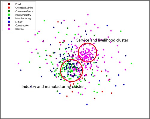
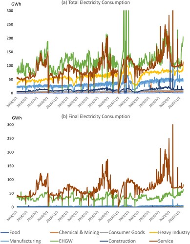
Based on the GB/T 4754-2017 specifications and our interpretations of sector descriptions, we organised the 440 sectors into eight sectors: food, chemical & mining, consumer goods, heavy industry, manufacturing, EHGW, construction, and service. We also decoded the specifications to determine whether the sectors are more strongly associated with final or intermediate consumption. In this context, the total production was calculated as the final plus intermediate production, similar to the construction of IO tables. The organised data are presented in Figure 2, where patterns of electricity consumption can be clearly observed. For instance, a drastic and persistent decrease in the total consumption of heavy industry and manufacturing industry was identified around February 2020, which is consistent with the lockdown measures imposed in Chongqing due to the COVID-19 outbreak. For a detailed specification of sector aggregation, please refer to the Supplementary Information.

Figure 2. Plots of chronological electricity consumption in eight sectors. The consumption is categorised into total and final consumption for the eight sectors according to their descriptions. Cyclical patterns can clearly be seen in the chronological datasets.

4. Results

4.1. Robustness testing

We sampled 500 days of the 971 total days with observations in the dataset to conduct model training. By comparing the outputs simulated with the trained model and all 471 remaining observations of the total outputs of the eight sectors, we produced Figure 3 to show the errors of both the statistical regression training and predictions in percentages. No significant change in error levels occurs after the training-prediction boundary is reached, suggesting that the model is effectively generalizable to unseen data and accurately captures the underlying relationship between the input variables and the target variable. In technical terms, overfitting occurs when the model learns the noise in the training data, leading to high accuracy for the training set but poor performance for the test set. Conversely, underfitting occurs when the model fails to capture the underlying patterns in the data, resulting in poor performance for both the training and test sets. The results indicate that the regressed model is influenced by neither overfitting nor underfitting, indicating that the model is likely to perform well in cases with new and unseen data. Some spikes can be seen across all eight sectors, which highly correspond to abnormal spikes in the actual data, as shown in Figure 2, suggesting that our model is able to filter out outliers among actual observations. This finding reinforces the robustness of our model and analysis.

Figure 3. The eight diagrams show the differences between the simulated and actual outputs of the eight sectors in percentages. To the left of the red dotted lines are the errors of the statistical regression model based on 500 historical observations. To the right of the red dotted lines are the errors of the predicted outcomes compared with the actual observations.

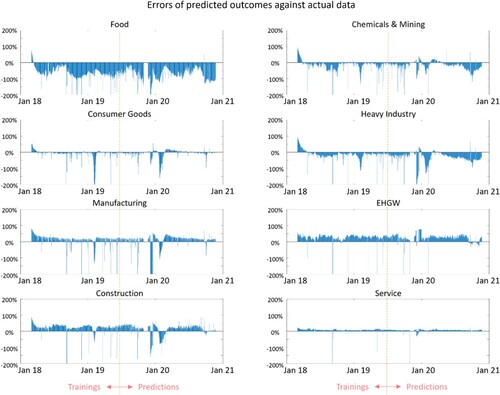
In addition, the error level is within −30% to 30% for most sectors, a tolerable value for ensuring the accuracy of the model. Among all eight sectors, the service sector has the lowest error level, while the food sector has the highest. A possible reason for the high error level of the food sector may be its significantly lower level of electricity consumption compared to other sectors. Throughout the 3-year observation period, the daily electricity consumption of the food sector never surpassed 0.5% of the daily total electricity consumption of the eight sectors. An unproportionally higher value of electricity consumption means that a higher level of noise is more likely to corrupt the information from the food sector. In other words, the food sector is affected by greater systematic error than other sectors, decreasing the accuracy of linkages modelled between the food sector and other sectors. Hence, caution should be taken when analysing food sector results in this specific case study. As proposed in signal process engineering, more advanced engineering may be needed to filter out noise and improve pattern recognition (Tuzlukov, 2018).

Moreover, as elaborated in the Data section, the I–O relationship revealed here using electricity consumption is not necessarily proportional to monetary input from the corresponding industry for the output sector, as described by the production coefficient $\mathbf{A}$ in the conventional IO Model. Table 2 quantitatively compares the differences between the production coefficients of the eight sectors in Chongqing obtained both from this research using the developed SIM algorithm and from the 2017 IO Table of Chongqing. For easier comparison, the ${\mathbf{A}}_{(t)}$ matrices are aggregated along the time horizon by summing all ${\mathbf{A}}_{(t)}$ into a single $\mathbf{A}$, mathematically represented as $\sum _{t=1}^8{\mathbf{A}}_{(t)}$. In Table 2(a), it should be noted that only nonnegative terms are kept in the aggregated $\mathbf{A}$ matrix for the same reason described in the Methods section. In addition, the sensitivity analysis in the previous paragraphs reveals that errors in the production coefficients exist. Both error sources contribute to the inaccuracy of Table 2(a), making some of the column sums of the aggregated $\mathbf{A}$ matrix larger than 1. Although apparent differences can be seen in the results of the two methods, some identical and key results can be observed. For instance, the total intermediate output from the heavy industry sector (the row sums of the heavy industry sector) is significantly larger than that from the other sectors in both sets of results. In addition, the contribution from the EHGW sector is significantly greater than that in the monetary IO table, possibly due to the adoption of electricity consumption as an indicator of all production activities.

Table 2. The input‒output production coefficients obtained (a) from the electricity consumption data in this research and (b) from the 2017 Input‒Output Table for Chongqing (a) Production coefficients for Chongqing obtained in this research from electricity consumption data.

	Food	Chemical & Mining	Consumer Goods	Heavy Industry	Manufacturing	EHGW	Construction	Service
Food	0.07	0.07	0.00	0.00	0.02	0.00	0.06	0.00
Chemical & Mining	0.08	0.02	0.00	0.04	0.02	0.01	0.08	0.00
Consumer Goods	0.07	0.04	0.03	0.02	0.01	0.01	0.07	0.00
Heavy Industry	0.17	0.30	0.48	0.71	0.56	0.00	0.01	0.00
Manufacturing	0.00	0.00	0.25	0.15	0.39	0.00	0.05	0.00
EHGW	0.00	0.82	0.00	0.58	0.00	0.16	0.11	0.00
Construction	0.07	0.04	0.11	0.07	0.00	0.01	0.09	0.01
Service	0.10	0.05	0.16	0.11	0.01	0.02	0.05	0.04
	Food	Chemical & Mining	Consumer Goods	Heavy Industry	Manufacturing	EHGW	Construction	Service
Food	0.06	0.00	0.04	0.00	0.00	0.00	0.01	0.00
Chemical&Mining	0.00	0.01	0.01	0.01	0.00	0.12	0.05	0.00
Consumer Goods	0.05	0.00	0.19	0.00	0.02	0.00	0.01	0.02
Heavy Industry	0.05	0.00	0.03	0.06	0.12	0.01	0.44	0.03
Manufacturing	0.01	0.00	0.01	0.00	0.31	0.01	0.06	0.02
EHGW	0.01	0.00	0.01	0.01	0.01	0.18	0.01	0.03
Construction	0.00	0.00	0.00	0.00	0.00	0.00	0.02	0.00
Service	0.09	0.01	0.08	0.02	0.08	0.07	0.15	0.18

To quantitatively compare the dissimilarity between the two production coefficient matrices, we adopted the methods of Avelino (2017). The two matrices yield a mean absolute deviation of 0.1124, mean absolute percentage error of 100.3366, weighted absolute percentage error of 2.6448, standardised weighted absolute difference of 0.9395, and PSI statistic of 4.5557. The significant differences show that the two matrices are indeed very distinct.

4.2. Chronological interlinkages of sectors

The SIM simulates how today’s production will induce further production in the future. With the electricity consumption data from Chongqing, we can reveal the chronological interactions among eight sectors in Chongqing or the ${\mathbf{A}}_{(t)}$ matrices explained in the Methods section. Due to the size of the ${\mathbf{A}}_{(t)}$ matrices, we are not able to present them in the main text. For readers’ reference, the complete ${\mathbf{A}}_{(t)}$ is included in the Supplementary Information. In ${\mathbf{A}}_{(t)}$, intermediate linkages are significantly larger when $t=1$, showing that most intermediate responses occur immediately after a demand signal is received. However, the EHGW sector demonstrates prolonged intermediate linkages to the chemical and mining sector at $8>t>1$, indicating that interactions between these two sectors take longer than interactions between other sector pairs.

To better depict the underlying concept, we plotted a Sankey diagram in Figure 4 to quantitatively illustrate the time lags in the induced production for one unit of demand (1 kWh in this case study) in the heavy industry sector. A detailed explanation of the derivation and construction of the Sankey diagram can be found in Table 1 and the corresponding paragraphs. From left to right, each of the eight columns in varied colours represents one calendar day as a production layer. The grey transparent bands connect the intermediate outputs and later outputs induced by them, with their widths proportional to the induced quantities. Hence, as explained in the Methods section and shown in Figure 4, when 1 kWh of final demand in the heavy industry sector is fulfilled, a market signal is sent out to induce a series of production events that propagate through the network across the eight sectors. A total of 7.73 kWh of output is generated throughout the eight sectors as a response to 1 kWh of demand in the heavy industry sector. This magnifying effect of demand can be inferred as the multiplier for the final demand of the heavy industry sector. The induced quantities decrease as the production layers extend into the future, in accordance with the logic that the multiplier impacts of the demand signal decay over time. In addition, the heavy industry sector induced the greatest production in the EHGW sector among all eight chronological layers (1.51 kWh, the sum of all bars labelled ‘EHGW' in Figure 4), which further induced a large proportion of outputs from the heavy industry sector (1.19 kWh, 79% of the 1.51 kWh of EHGW electricity consumption induced), illustrating the close connection between EHGW and heavy industry.

Figure 4. Sankey diagram showing the chain of responses to one unit of demand in heavy industry in all eight sectors. Bars in different colours and with different codes indicate the scale of electricity consumption and economic outputs in the respective chronological production sector. The label below each column indicates the number of layers delayed for that column. The bands connect the intermediate outputs and later outputs induced by them. The scales of the bands and columns are proportional to the scale of electricity consumption/economic outputs induced. Transactions less than 0.01 kWh are omitted for visual clarity.

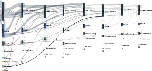
In comparison, the food sector is the least associated with the heavy industry sector, with 0.08 kWh (the sum of all bars labelled with F in Figure 4) of output induced from the 1 kWh of final demand from the heavy industry sector. The impact of the food sector output in layer 1 does not extend far into the future, with less than 0.01 kWh of output induced in layer 2 of heavy industry, as highlighted in red in Figure 4. Furthermore, it can be observed that the service sector induced outputs into the more distant future, a feature not seen in sectors such as the food, consumer goods, and chemical sectors. The 0.1 kWh demand of the service sector in layer 1 induced 0.01 kWh of output in layer 6 of the heavy industry sector, almost equivalent to the induced output in layer 2 of the heavy industry sector, as shown by the branches highlighted in blue in Figure 4. This may result from the longer logistic chain and, thus, longer duration of demand signal propagation in the service sector, which is an interesting takeaway of our analysis.

The size of the vertical bars in Figure 4 also conveys valuable insights derived from the trained model. In the first layer, a total output of 1.67 kWh is produced. However, in the second layer, the output decreases to a mere 0.76 kWh. Interestingly, none of the layers following the first layer exhibit sizes larger than that of the second layer. This observation suggests that the required electricity outputs decrease as time progresses into the future, a phenomenon that is consistent with the physical performance of the economic system.

Since the information from the Sankey diagram is too abundant to be fully analysed here, we have included the data used to construct Figure 4 in the Supplementary Information. In the Supplementary Information, together with an analysis of the heavy industry, we present the same chronological outputs given a 1 kWh demand from the seven other sectors. However, it should be noted that the chronological lag between sectors should not be considered equivalent to the transmission time from one sector to another. This is because the time needed for one sector to respond to the demand change in another may be a result of interactions among multiple factors, including the nature of the industry, the size of the business, the availability of effective communication channels, etc. Depending on the context, transportation may not play a role in determining the time delay, as businesses can react to market signals with their inventories to conduct production. On the other hand, the service sector, for instance, may naturally adjust its production level much quicker in response to market signals, as they rely less on inventory build-up in comparison.

4.3. Scenario predictions

The chronological coefficients obtained, as discussed in the previous section, can be used to predict the multiplier effects in all sectors given forecasts of the final demand changes in one sector. We varied the daily growth rate of final demand for consumer goods and made forecasts of the daily outputs of all eight sectors for the next 80 days. We chose 80 days as the prediction boundary to avoid systematic uncertainties that may not be captured by our modelling. For instance, our model cannot capture the impact of sudden changes, such as disaster events, on capital equipment, as the model assumes unchanged productivity.

Figure 5 effectively illustrates the prediction results for various scenarios. In each of these scenarios, the historical observations can be observed to the left of the distinct red dotted lines, while the predictions extending 80 days into the future are displayed to the right of these same red dotted lines. As part of the scenario-setting process, we altered the forecast of the daily growth of final consumption in the consumer goods sector, ranging from an increase of 0.41% to a decrease of −0.40% for the surging and plunging scenarios, respectively. These adjustments were based on the careful calculation of past data variances. For the baseline scenarios, we derived the mean growth rates of final demand for all sectors by meticulously analysing historical calculations. At the end of the 80-day prediction period, the calculated model predicted a difference of 3.5 GWh/day in the mean value of total electricity consumption within the consumer goods sector. Intriguingly, while the final consumption levels in the surging and plunging scenarios remained unchanged, the heavy industry (with a difference of 18.8 GWh/day), manufacturing (with a difference of 6.8 GWh/day), and EHGW (with a difference of 11.7 GWh/day) sectors exhibited more significant differences in the mean values of their forecasted total electricity consumption on the 80th day compared to that for the consumer goods sector. From this observation, we can deduce that any fluctuations in the final demand for consumer goods tend to have a more pronounced impact on these three sectors than on other sectors.

Figure 5. The simulated outputs/electricity consumption of eight sectors under three scenarios of growth in the consumer goods sector, plotted with error ranges. The daily growth rates of sectors are estimated based on historical means and variances, but the mean growth rate of the consumer goods sector is varied to simulate the changes across all sectors under the three scenarios. To the right of the red dotted lines, the coloured areas show the error ranges, while the black solid lines show the predicted mean outputs.

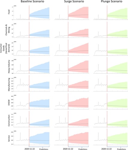
On the other hand, when comparing the differences in total electricity consumption across various sectors under the plunging and surging scenarios in proportion to the baseline scenario, the trained model reveals that the most substantial relative difference in total electricity consumption occurs within the consumer goods sector, at 43%. The heavy industry and manufacturing sectors exhibit the next-largest relative difference for these scenarios, at 21% each. In contrast, the EHGW sector, with a 13% relative difference, is the sector with the second smallest relative difference after displaying the third largest absolute difference. The disparity between absolute and relative measurements may be attributed to the varying energy intensities in different sectors. For instance, the EHGW sector is naturally energy intensive, while other sectors, such as service sectors, utilise less energy in their production processes. As a result, the absolute measurement may be more appropriate for predicting the electricity consumption required in each respective sector. Conversely, relative measurements can serve as a good indicator of changes in economic activity levels.

5. Conclusion and discussion

In this research, we used the SIM to explore the possibility of reconciling modelling and regression analysis. Since electricity consumption is a good approximation of economic activities, the promising results of this research can be directly applied to local economic planning. For instance, the revealed chronological interconnections among sectors can help us better understand the industrial symbiosis among sectors, thus helping to predict the impacts of external shocks on final demand. Integrating economic modelling and statistical algorithms can support emerging computational science, a third approach to scientific exploration in addition to theoretical and experimental science. From weather forecasting to mechanical design, computational science has proven incredibly useful in providing effective solutions at a significantly reduced cost. The availability of massive datasets and improvements in computational power support scientific research by providing a sound basis for the validation of theories and models, as well as enabling analyses that were previously impossible without emerging computational tools. This research demonstrates the successful application of computational science in the field of economics, showcasing the potential of harnessing advanced technology to gain deeper insights into complex economic systems and inform decision-making processes.

Specifically, the algorithm proposed for the SIM is designed to analyse the economic structure of a region across various sectors over time. Sufficient data on economic performance are plugged into the model to identify the chronological interdependencies within the economy. This enables the ‘nowcasting’ of economic output by sector, providing vital information for decision-makers. Such insights are crucial for establishing quick policy responses to economic shocks and mitigating direct and indirect economic losses through effective resource allocation and intervention strategies.

Nevertheless, some additional technical improvements could further enhance our algorithm in future studies. For example, in this study, the number of layers for production propagation is set to only eight due to computational power limitations. Thus, upgrading computer hardware may further improve the accuracy of the results in this research as well as any future research that adopts our algorithm. In addition, it may be useful to integrate real-world surveys on supply chains for reference when determining the number of layers. Alternatively, knowledge of engineering processes, geolocations, and infrastructure capacities may aid in modelling delays in propagation between different sectors. Access to such information may also improve over time with the increased availability of big data from various sources.

Furthermore, the classification of the final demand and intermediate output in this research is based on empirical judgement. For instance, due to possible misinterpretations and misinformation provided by consumers, systematic error may be embedded in the data used in this research and thus deteriorate model performance. Technical signal processing methods, such as noise filtering, can improve the accuracy of data analysis and thereby enhance model performance.

In addition, in the study of Romanoff and Levine (1981), a detailed explanation and a comprehensive discussion were provided regarding the difference between anticipatory and responsive demands. In all the simulations conducted in this study, responsive demands were assumed. Thus, intermediate production only responded to demands that had already occurred. In real-world situations, this assumption may not always hold, as some changes in production activities will occur before a change in actual demand is observed through market forecasting and speculation.

Finally, the SIM is an oversimplified economic model in which the nonlinear effects of variables such as capital constraints and price elasticity are not considered. Although the simple and linear features of the SIM provide efficient estimates for production coefficients in the short term, nonlinearity should be considered to further develop the SIM and incorporate more economic theories in the next stages of modelling. Therefore, it may be interesting to look at the hybridisation of control system engineering and economic modelling. The nonlinear modules in control systems can be used to model the nonlinear feedback effects of certain sectors in the whole economy. In this regard, the SIM could be deemed as a system identification model, but without a black box structure, thus supporting research on and analyses of chronological processes. Further developments may push the frontier of integrated economic-cybernetic research.

Acknowledgements

Zhifu Mi acknowledges support from the Engineering and Physical Sciences Research Council (EP/V041665/1). Jinkai Li acknowledges support from the National Social Science Foundation of China (20BJL034). We would like to express our gratitude to Prof. Yasuhide Okuyama, Editor of Economic Systems Research, for the constructive comments and advice during the publication process. Prof. Okuyama’s critical observation and detailed responses has significantly refined our work. We would also like to extend our thankfulness to the anonymous reviewers for their comments and suggestions to the manuscript.

Disclosure statement

No potential conflict of interest was reported by the author(s).

Additional information

Funding

This work was supported by Engineering and Physical Sciences Research Council [grant number: EP/V041665/1]; National Social Science Fund of China [grant number: 20BJL034].

References

- Ashraf, Z., Javid, A. Y., & Javid, M. (2013). Electricity consumption and economic growth: Evidence from Pakistan. Economics and Business Letters, 2(1), 21–32. https://doi.org/10.17811/ebl.2.1.2013.21-32
- Aslan, A., Apergis, N., & Yildirim, S. (2014). Causality between energy consumption and GDP in the U.S.: evidence from wavelet analysis. Frontiers in Energy, 8(1), 1–8. https://doi.org/10.1007/s11708-013-0290-6
- Avelino, A. F. T. (2017). Disaggregating input–output tables in time: The temporal input–output framework. Economic Systems Research, 29(3), 313–334. https://doi.org/10.1080/09535314.2017.1290587
- Crown, W. H. (2019). Real-world evidence, causal inference, and machine learning. Value in Health, 22(5), 587–592. https://doi.org/10.1016/j.jval.2019.03.001
- Dong, X. S., Qian, L. J., Huang, L., & IEEE. (2017). A CNN based bagging learning approach to short-term load forecasting in smart grid. 2017 IEEE smartworld, ubiquitous intelligence & computing, advanced & trusted computed, scalable computing & communications, cloud & big data computing, internet of people and smart city innovation (Smartworld/Scalcom/Uic/Atc/Cbdcom/Iop/Sci).
- Einav, L., & Levin, J. (2014). Economics in the age of big data. Science, 346(6210), 1243089. https://doi.org/10.1126/science.1243089
- Fezzi, C., & Fanghella, V. (2020). Real-time estimation of the short-run impact of COVID-19 on economic activity using electricity market data. Environmental and Resource Economics, 76(4), 885–900. https://doi.org/10.1007/s10640-020-00467-4
- Hamermesh, D. S. (2013). Six decades of top economics publishing: Who and How? Journal of Economic Literature, 51(1), 162–172. https://doi.org/10.1257/jel.51.1.162
- Harding, M. C., & Lamarche, C. (2021). Small steps with Big Data: Using machine learning in energy and environmental economics. Annual Review of Resource Economics, 13(1), 469–488. https://doi.org/10.1146/annurev-resource-100920-034117
- Hastie, T., Tibshirani, R., & Friedman, J. (2009). The elements of statistical learning: Data mining, inference, and prediction.
- He, K., Mi, Z., Coffman, D. M., & Guan, D. (2022). Using a linear regression approach to sequential interindustry model for time-lagged economic impact analysis. Structural Change and Economic Dynamics, 62, 399–406. https://doi.org/10.1016/j.strueco.2022.03.017
- Janzen, B., & Radulescu, D. (2020). Electricity use as a real-time indicator of the economic burden of the COVID-19-related lockdown: Evidence from Switzerland. CESifo Economic Studies, 66(4), 303–321. https://doi.org/10.1093/cesifo/ifaa010
- Kim, Y. S. (2015). Electricity consumption and economic development: Are countries converging to a common trend? Energy Economics, 49, 192–202. https://doi.org/10.1016/j.eneco.2015.02.001
- Leontief, W. W. (1953). Studies in the structure of the American economy. Oxford University Press.
- Levine, S. H., & Romanoff, E. (1989). Economic impact dynamics of complex engineering project scheduling. IEEE Transactions on Systems, Man, and Cybernetics, 19(2), 232–240. https://doi.org/10.1109/21.31029
- López Prol, J., & O, S. (2020). Impact of COVID-19 measures on short-term electricity consumption in the most affected EU countries and USA states. iScience, 23(10), 101639. https://doi.org/10.1016/j.isci.2020.101639
- Ludwig, N., Feuerriegel, S., & Neumann, D. (2015). Putting Big Data analytics to work: Feature selection for forecasting electricity prices using the LASSO and random forests. Journal of Decision Systems, 24(1), 19–36. https://doi.org/10.1080/12460125.2015.994290
- Mellander, C., Lobo, J., Stolarick, K., & Matheson, Z. (2015). Night-time light data: A good proxy measure for economic activity? PLoS One, 10(10), e0139779. https://doi.org/10.1371/journal.pone.0139779
- Mullainathan, S., & Spiess, J. (2017). Machine learning: An applied econometric approach. Journal of Economic Perspectives, 31(2), 87–106. https://doi.org/10.1257/jep.31.2.87
- Naimur Rahman, M., Esmailpour, A., & Zhao, J. (2016). Machine learning with Big Data An efficient electricity generation forecasting system. Big Data Research, 5, 9–15. https://doi.org/10.1016/j.bdr.2016.02.002
- Novan, K., Smith, A., & Zhou, T. (2020). Residential building codes do save energy: Evidence from hourly smart-meter data. The Review of Economics and Statistics, 104(3), 483–500. https://doi.org/10.1162/rest_a_00967
- Okuyama, Y., Hewings, G. J. D., & Sonis, M. (2004). Measuring economic impacts of disasters: Interregional input-output analysis using sequential interindustry model. In Y. Okuyama & S. E. Chang (Eds.), Modeling spatial and economic impacts of disasters (pp. 77–101). Springer Berlin Heidelberg.
- Okuyama, Y., Hewings, G. J., & Sonis, M. (2000). Sequential interindustry model (SIM) and impact analysis: application for measuring economic impact of unscheduled events. 47th north American meetings of the regional science association international, Chicago, IL.
- Perez-Chacon, R., Asencio-Cortes, G., Martinez-Alvarez, F., & Troncoso, A. (2020). Big data time series forecasting based on pattern sequence similarity and its application to the electricity demand. Information Sciences, 540, 160–174. https://doi.org/10.1016/j.ins.2020.06.014
- Qu, H. N., Ling, P., & Wu, L. B. (2015). . Electricity consumption analysis and applications based on smart grid Big Data. IEEE 12th Int Conf Ubiquitous Intelligence & Comp/IEEE 12th Int Conf Adv & Trusted Comp/Ieee 15th Int Conf Scalable Comp & Commun/IEEE Int Conf Cloud & Big Data Comp/IEEE Int Conf Internet People and Associated Symposia/Workshops, 923–928.
- Romanoff, E., & Levine, S. H. (1977). Interregional sequential interindustry modeling: A preliminary analysis of regional growth and decline in a two region case. Northeast Regional Science Review, 7, 87–101.
- Romanoff, E., & Levine, S. H. (1981). Anticipatory and responsive sequential interindustry models. IEEE Transactions on Systems, Man, and Cybernetics, 11(3), 181–186. https://doi.org/10.1109/TSMC.1981.4308650
- Romanoff, E., & Levine, S. H. (1990). Combined regional impact dynamics of several construction megaprojects. Regional Science Review, 17, 85–93.
- Šćepanović, S., Mishkovski, I., Hui, P., Nurminen, J. K., & Ylä-Jääski, A. (2015). Mobile phone call data as a regional socio-economic proxy indicator. PLoS One, 10, e0124160.
- Tuzlukov, V. (2018). Signal processing noise. CRC Press.
- UN. (2008). International Standard Industrial Classification of all Economic Activities (ISIC - Rev. 4). Retrieved February 19, 2017, from https://unstats.un.org/unsd/cr/registry/isic-4.asp
- Varian, H. R. (2014). Big data: New tricks for econometrics. Journal of Economic Perspectives, 28(2), 3–28. https://doi.org/10.1257/jep.28.2.3
- Viloria, A., Sierra, D. M., Camargo, J. F., Zea, K. B., Fuentes, J. P., Hernandez-Palma, H., & Kamatkar, S. J. (2020). Demand in the electricity market: Analysis using Big Data. Intelligent Computing, Information and Control Systems, Iciccs 2019, 1039, 316–325. https://doi.org/10.1007/978-3-030-30465-2_36
- Wang, Z. Y., Ye, X. Y., Lee, J., Chang, X. M., Liu, H. M., & Li, Q. Q. (2018). A spatial econometric modeling of online social interactions using microblogs. Computers, Environment and Urban Systems, 70, 53–58. https://doi.org/10.1016/j.compenvurbsys.2018.02.001
- Yuan, Y. H., Tsao, S. H., Chyou, J. T., & Tsai, S. B. (2020). An empirical study on effects of electronic word-of-mouth and Internet risk avoidance on purchase intention: From the perspective of big data. Soft Computing, 24(8), 5713–5728. https://doi.org/10.1007/s00500-019-04300-z
- Zeng, A. R., Liu, S., & Yu, Y. (2019). Comparative study of data driven methods in building electricity use prediction. Energy and Buildings, 194, 289–300. https://doi.org/10.1016/j.enbuild.2019.04.029
- Zhang, C., Zhou, K., Yang, S., & Shao, Z. (2017). On electricity consumption and economic growth in China. Renewable and Sustainable Energy Reviews, 76, 353–368. https://doi.org/10.1016/j.rser.2017.03.071
- Zhou, K., Yang, C., & Shen, J. (2017). Discovering residential electricity consumption patterns through smart-meter data mining: A case study from China. Utilities Policy, 44, 73–84. https://doi.org/10.1016/j.jup.2017.01.004