Inequality and Exchange Rate Movements in an Open-Economy Macroeconomic Model

ABSTRACT

This article presents a complete macroeconomic (SFC) model to study income and wealth distribution in an open economy. We argue that exchange rates and the stock of foreign debt play a major role in shaping inequality across and within countries. Using the ‘relative income hypothesis’, we show that debt-financed consumption of low-income households can affect both total income and the disposable income of high-income households in the medium run. In addition, while higher inequality is detrimental to the domestic economy, it can benefit trading partners.

KEYWORDS:

• Open economy
• inequality
• foreign investments
• stock-flow consistency

JEL CODES:

• E17
• E21
• F31
• F32
• F41

1. Introduction

The relationship between finance and inequality has attracted increasing attention since the beginning of the United States’ financial crisis in 2007–08. The topic has often been framed within with the broader concept of ‘financialisation’.

Most studies focus on single countries or areas. As a result, the role of cross-country capital flows and exchange rates is usually neglected. We present an open economy model, named IEROE (Inequality and Exchange Rate in the Open Economy), which aims at bridging this research gap. Its basic structure is derived from the OPENFLEX model developed by Godley and Lavoie (2007). The benchmark model has been augmented by three blocks of equations. The new features are as follows: (1) each domestic household sector is divided into two groups, based on their median income; (2) low-income households try to emulate high-income households’ consumption patterns (relative income hypothesis, RIH); and (3) consumer credit of low-income households is funded by bank loans.

The article is organised as follows. Section Two presents the concept of ‘financialisation’ and provides evidence on how it has been used to summarise a coherent series of ‘structural socio-economical changes’. Section Three features a literature review on most recent contributions on finance and inequality. Model structure is discussed in detail in Section Four. In Section Five we use the model to test the impact of emulative behaviour and a change in the primary distribution of income, respectively. We show (experiment 1) that low-income households’ emulative behaviour (funded by bank loans) has a medium-run negative impact on total domestic income. In addition, it affects income and net financial wealth of the upper class. A more unequal distribution of income (experiment 2) is detrimental for the country as a whole. However, it can benefit both high-income domestic households and trading partners. In Section Six, we show that model results replicate the available time series for the US economy throughout the 2007–08 crisis. More generally, our experiments shed light on the main causal relationships between growing income and wealth inequality and financial instability in an open economy. This can also prove itself very useful in the economics of the Covid-19 pandemic, as evidence is emerging that the recent economic shock has contributed to a further increase in the level of cross-country inequality (Bottan, Hoffmann, and Vera-Cossio 2020; Nassif-Pires et al. 2020; Qureshi 2020; Perry, Aronson, and Pescosolido 2021). Post-pandemic recovery plans should take this lesson into account if they want to contribute to a more stable and resilient economy. Final remarks are provided in Section Seven.

2. The Context: Financialisation

The term ‘financialisation’ is often used to mark the period from the late 1970s to the outbreak of the crisis of 2007–08. Many authors have used the term in exploring various aspects of advanced economies ever since ‘but the literature on financialisation is at present a bit of a free-for-all, lacking a cohesive view of what is to be explained’ (Krippner 2005, p. 181). In fact, more than 15 years later, a unique interpretation of this concept in the economic literature is still lacking.

According to Epstein (2019, p. 380), financialisation ‘refers to the increasing importance of financial markets, financial motives, financial institutions, and financial elites in the operation of the economy and its governing institutions, both at the national and international level’. This definition is sufficiently general to include a variety of structural changes that occurred in most advanced economies. In the next subsections, we briefly discuss some of the most relevant changes.

2.1. Changes in the Distribution of Income

During the financialisation era, the distribution of income has favoured capital over labour (see Hein and Dodig 2015 for a long-run analysis of this phenomenon). Figure 1 shows the evolution of the functional distribution of income in selected economies. Figure 2 focuses on the top 1 per cent income share.

Figure 1. Labour share of national income (%). Selected OECD countries.

Note: Our elaboration on World Inequality Database data, 2021.

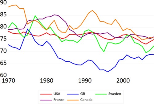
Figure 2. Pre-tax national income, share of top 1 per cent. Selected OECD countries.

Note: Our elaboration on World Inequality Database data, 2021.

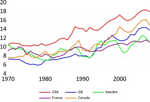
All the countries have recorded a decrease in the wage share since the late 1970s. Most of the ‘redistribution’ took place during the 1980s. At the same time, the earnings of the top 1 per cent income share recorded substantial growth. This bottom-up redistribution of income started in the early 1980s in the US and UK, where Ronald Reagan and Margaret Thatcher spearheaded the ‘conservative revolution’ in the western world. In Spain, Germany, Sweden and France, this redistribution process only started in the mid-1990s or even the early 2000s (Hein 2015).

The more unequal distribution of income between wages and profits (including dividends, interest payments, and retained profits) went along with a more unequal distribution of personal income among the wage earners (that is, between low-income workers and top managers, sport and showbusiness stars, and employees of the financial sector). The falling bargaining power of the trade unions and the change in the structure of the economy has contributed to the stagnation of real wages in the traditional manufacturing industries.

2.2. Financialisation of the Firms

Non-financial firms have increased their portfolio investments in the stock markets and opened new financial subsidiaries rather than purchasing new machinery and plants (Dodig and Hein 2015). The share of financial incomes of firms has increased since the early 1980s. Figure 3 shows the level of financial assets as a percentage of tangible assets for US non-financial corporations. The level of financial assets held by non-financial corporations has increased constantly compared to the level of tangible assets. Figure 4 shows the level of ‘financial income’ received by non-financial corporations as a percentage of the internal funds held by the firms. The figures are a good summary of the shift towards ‘financial management’ undertaken by non-financial firms since the end of the 1970s.

Figure 3. Financial assets as a percentage of total assets, non-financial corporations. United States.

Note: Our elaboration on FRED data, 2021.

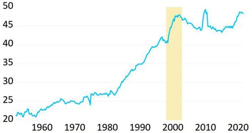
Figure 4. Dividends to undistributed profits ratio (%), non-financial corporations. United States.

Note: Our elaboration on US Bureau of Economic Analysis (BEA) data, 2021.

2.3. Financial Liberalisation and Debt-Financed Consumption

The increasing availability of consumer credit during the financialisation era has created the conditions for debt-financed consumption. At the same time, increasing income inequality has fostered trickle-down consumption. Indeed, the concentration of income and wealth has encouraged low-income consumers to mimic the consumption behaviours of the wealthy. This relative income hypothesis (RIH) traces back to the seminal work of Duesenberry (1949), which, in turn, echoes Veblen’s (1899) institutionalist approach. It underlines the importance of habit formation and emulative behaviour in the consumption patterns of different social groups (‘keeping up with the Joneses’). Building upon Duesenberry (1949), Frank, Levine, and Dijk (2014) have proposed the so-called expenditure cascades hypothesis. The latter aims at explaining the decline in the observed savings rate in the US during the financialisation period via a cascade mechanism: higher household expenditure in the top income quintile (or decile) leads households from the second to the top quintile to spend more. Imitation, in turn, drives up the consumption of households in the third to the top quintile, and so on.

In some cases, the private debt-financed boom has offset the contractionary impact of the shift in income distribution in favour of the richer part of the population, and the depressive effect of the decline in net investment of production firms.

In addition, new financial norms, new financial instruments and new financial practices have lowered creditworthiness standards. These changes — usually named ‘financial liberalisation’ — have also encouraged lending to the household sector. This specific aspect of financialisation is the subject of the first experiment in Section Four.

2.4. Exchange Rate and Capital Account Liberalisation

Another dimension of financial liberalisation involves changes in interest rate controls and restrictions on international financial transactions. A stronger cross-country financial interconnection is another feature of the financialisation era. Capitals have been allowed to move more freely from one country to another. International investors have started to engage in ‘carry trade’ operations or interest arbitrage (borrowing in one currency to invest, or lend, in another). Perceptions of possible devaluations have often led to large capital outflows, thus fostering exchange-rate crises (Stockhammer 2010). The new ‘financial interconnection’ at the international level allowed some countries, especially the US, to run chronic current account deficits. This requires attracting large capital inflows, which, in turn, rest on capital account liberalisations.

2.5. Financial Development

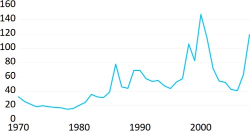
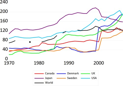
The distinction between financial liberalisation and financial development was first proposed by Abiad, Oomes, and Ueda (2008). The latter includes both the extension of financial services to new users (extensive margin) and the improvement of the quality of financial services for old users (intensive margin). Financial development is often measured by total credit (to the private sector) to GDP ratio. Figure 5 shows the dramatic increase of financial development at an international level during the financialisation era, with periods of abrupt acceleration in some countries (the UK in the mid-1980s and Sweden in the late 1990s).

Figure 5. Domestic credit to private sector (% of GDP). Selected OECD countries.

Note: Our elaboration on World Bank data, 2021.

2.6. Debt-Led vs Export-Led Growth Regimes

The combination of the points made in Sections 2.3 (debt-finance consumption) and 2.4 (capital account liberalisation) has generated a typical growth pattern often described as the debt-led private demand boom regime. In particular, the US has relied on an increasing role of consumption in sustaining domestic demand. However, this has generated a higher demand for foreign goods, thus fostering export-led complementary growth regimes (such as those in Germany, Japan, and Sweden). In turn, external surpluses of export-led economies have been invested in the debt of the United States and other deficit counties, thanks to capital account liberalisation.

An export-led regime can also originate from the poor dynamics of some autonomous aggregate demand components, namely, government spending, instead of growing inequality or the growing power of finance. Still, the imbalances that are generated by these uneven growth patterns can be sustained only in the presence of some degree of financial liberalisation and financial development, as the recent history of the Euro Area has shown.

However, the relationship between these different growth regimes is more complex then usually recognised. In Section Four, we show that, counter-intuitive though it may sound, the end of a debt-led growth regime in one country does not have the same (long-term) negative effect on its trading partners.

3. Literature Review

The structural changes presented in Section Two have been analysed in several works. They usually focus on how, and to what extent, different financialisation dimensions have affected each other.

Many empirical studies point to financial development as a major cause of income inequality in both advanced economies and developing countries (e.g., Jauch and Watzka 2012; Jaumotte, Lall, and Papageorgiou 2013; Van Arnum and Naples 2013; Li and Yu 2014; Dabla-Norris et al. 2015; Denk and Cournede 2015; Hein 2015; Godechot 2016; Dünhaupt 2017). Financial liberalisation is also associated with income inequality by Jaumotte and Osorio Buitron (2015) and Hein (2015). In addition, de Haan and Sturm (2017) use a panel fixed-effect model with 121 countries (covering 1975–2005). They find that all financial variables contribute to increasing income inequality. Hein et al. (2018) identify three channels whereby financialisation boosts income inequality (sector composition of the economy, overhead costs, and trade union bargaining power). They test how the Global Financial Crisis has affected the financialisation–distribution nexus in three member states of the Euro Area (notably, Spain, Germany, and France).

Some works focus on the specific characteristics of financialisation in non-financial industries. For instance, agriculture financialisation — meaning a process that drives prices away from levels determined by non-speculative demand and supply conditions — can have a dramatic impact on poverty via food supply and income fluctuations, especially in developing countries (e.g., Aït-Youce 2019; Ouyanga and Zhang 2020).

Other studies reverse the causation direction. For instance, it has been argued that the Global Financial Crisis was generated by the rising inequality of income and wealth since the end of the 1990s (e.g., Dosi et al. 2013; van Treeck 2014; Kumhof, Ranciere, and Winant 2015; Stockhammer 2015; Russo, Riccetti, and Gallegati 2016). Other authors stress the importance of low-income households’ demand for loans (e.g., Fitoussi and Saraceno 2010; Rajan 2010; Cynamon and Fazzari 2013). There are also works that focus on the demand for more sophisticated financial products on the part of the upper class, which seeks more lucrative portfolio investments (e.g., Lysandrou 2011; Goda and Lysandrou 2014).

Kumhof et al. (2012) develop an open-economy dynamic stochastic general equilibrium (DSGE) model, in which current account imbalances can arise in response to rising domestic income inequality. The model features an economy with two classes of household: investors, who own the capital stock of the economy and lend money through the financial markets; and workers, who borrow to fund a level of spending that is greater than the income they receive.

Kapeller and Schutz (2014) present a stock-flow consistent (SFC) model whereby the interaction between households’ ‘conspicuous consumption norms’ and banks’ loosening credit standards can generate instability, that is, a ‘Minsky–Veblen cycle’.

D’Orazio (2019) studies the effects of rising inequality on household debt, financial fragility, and macroeconomic instability using an agent-based stock-flow consistent (AB-SFC) model for a closed economy. Similarly, Botta et al. (2021) use an AB-SFC model to investigate the complex relation between financialisation and inequality, assuming no predetermined causation.

Turning to the RIH, its rediscovery dates back to the early 1970s. After a period of oblivion, due to the popularity of Friedman’s permanent income hypothesis (Friedman 1957), the RIH has been used by Krelle (1972), Gaertner (1974), Pollak (1976), Hayakawa and Venieris (1977), Douglas and Isherwood (1978), and Frank (1985).

More recently, Christen and Morgan (2005) have argued that increasing income inequality has created the need for low- and middle-income households to borrow in order to ‘keep up’ their consumption level in line with the ‘norm’. The widespread use of borrowing to consume more than disposable income was enabled by a loosening in bank credit standards and the surge in the value of residential-estate assets. According to Bhaduri (2011), this is a typical dynamic of a financial crisis of domestic origin. Bhaduri (2011, p. 996) develops a formal model of debt cycles in which the Global Financial Crisis is used ‘as a background’. Higher asset prices push up the ‘notional’ wealth of households. They can keep borrowing by using more and more valuable assets as collateral. Additional spending ensues, reinforcing asset bubble growth. The private debt-financed boom offsets the contractionary impact of the shift in income distribution in favour of the upper class, and the depressive effects of the decline in production firms’ net investment. In addition, new financial norms, new financial instruments, and new financial practices (such as the securitisation of mortgages and other types of debt) contribute to lower creditworthiness standards (Bhaduri 2011).

The expenditure cascades hypothesis has been put forward by Frank, Levine, and Dijk (2014). The transmission mechanism from higher levels of inequality to generalised lower saving rates is presented through a theoretical model and computer simulations. Regressions on US data are also used to provide empirical support to the theory.¹ Given the unavailability of figures on household saving rates for different levels of income at a state or county level, regressions are performed using various indicators of financial distress as dependent variables (i.e., the number of bankruptcies, divorce rates, travel time to work, etc.). In fact, the RIH is tested via the use of a hypothesis proxy, that is, that ‘families living in high-inequality areas will find it harder to live within their means than their counterparts in low-inequality areas’ (Frank, Levine, and Dijk 2014, p. 63). The strong correlation between inequality and financial distress shown by their model chimes with the results of other research on the impact of inequality on total hours worked (Bowles and Park 2005) and median house prices (Ostvik-White 2003).

The RIH has been used in stock-flow consistent models, too. Detzer (2018) tests the effects of a change in the functional distribution of income, and in wage dispersion, on two stylised economies that differ only in their respective emulation coefficients. The foreign sector is considered, but exchange rates and terms of trade are ignored. Cardaci and Saraceno (2016) use the expenditure cascades hypothesis in an AB-SFC model for a closed economy. Belabed, Theobald, and van Treeck (2018) use a three-country SFC model (including the US, China, and Germany). Both the export-led growth of the economies of China and Germany and the credit-led growth of the US economy (before the Global Financial Crisis) are generated by a bottom-up redistribution of domestic incomes. Exchange rates are treated as exogenous variables (using observed time series) and international financial transactions are not modelled (except for foreign loans to households). Hein and Dodig (2015) analyse debt-led versus export-led growth dualism as the by-product of financialisation and inequality. Finally, Behringer and van Treeck (2019) use a sectorial balance approach to study whether (and how) different patterns of change in income distribution (i.e., changes in functional income distribution versus changes in personal income distribution) have generated different growth models through the emergence of current account imbalances.

Our work innovates with respect to the aforementioned literature as it links inequality and imitative behaviours with changes in the exchange rate and cross-country capital flows within a stock-flow consistent model. The research questions we aim at addressing here are: what is the nexus, if any, between income (and wealth) distribution and capital flows under a floating exchange rate regime (that is, when foreign portfolio investments are driven by exchange rate adjustments)? How does distribution affect cross-country economic performance via exchange rates and foreign portfolio investment adjustments? What are the effects of a boom-and-bust cycle in one country on its trading partners? Are debt-led and export-led regimes mutually interdependent, as is usually believed?

In our model, the relation between income patterns and economic growth is not dominated by the negative effects of bottom-up income redistribution on domestic demand. We argue that international flows of capital and exchange rate adjustments play a crucial role. In other words, our findings do not depend on differences in marginal propensities to consume across different social groups. Rather, long-term negative effects of income inequality are explained by the detrimental impact of a stronger currency on the competitiveness of the country and its international investment position. In addition, paradoxical though it may sound, a debt-led boom and more equal distribution may have a detrimental impact on trading partners. Similarly, a lower level of income in one country can benefit the others, once international flows of capital and exchange rate adjustments are factored in. International trade can actually become a zero-sum game.

4. The Model

We use a two-country dynamic macroeconomic stock-flow consistent model. It is a revised version of the OPENFLEX model developed by Godley and Lavoie (2007). The two economies considered are roughly the same size. Coefficients and initial values of endogenous variables are set borrowing from the literature and/or using reasonable values, based on the empirical evidence. Overall, the model is calibrated in such a way as to reproduce the available time series for the US and the Euro Area, respectively. The terms of trade are ruled by a floating exchange rate regime.

The model is made up of 101 equations, including 45 accounting identities, 10 equilibrium conditions, and 21 behavioural equations. We refer the reader to the Appendix for a complete list of equations, variables, and parameter values. Parameters and exogenous variables are in bold characters.

The balance sheet and the transaction flow matrix of the economy are displayed in Table 1 and Table 2, respectively. Table 1 shows that there are six types of asset and liability: money (cash), domestic deposits, domestic government bills, foreign government bills, and loans and advances (from the central bank to commercial banks). For the sake of simplicity, gross investment in fixed capital is modelled assuming that firms invest as long as the actual capital stock is below the desired capital to output ratio. Once the desired capital stock is achieved, they invest only to cover depreciation.

Table 1. Balance sheet matrix.

	Euro Area							United States
	Rich households	Poor households	Production firms	Government	Commercial banks	Central bank		Rich households	Poor households	Production firms	Government	Commercial banks	Central bank	Sum
Money	$+H_r^{\text{€}}$	$+H_p^{\text{€}}$				$-H^{\text{€}}$	$x{r}_{\text{€},\mathrm{\$}}$	$+H_r^{\mathrm{\$}}$	$+H_p^{\mathrm{\$}}$				$-H^{\mathrm{\$}}$	$0$
Deposits	$+\mathrm{De}{p}_r^{\text{€}}$	$+\mathrm{De}{p}_p^{\text{€}}$			$-\mathrm{De}{p}_b^{\text{€}}$			$+\mathrm{De}{p}_r^{\mathrm{\$}}$	$+\mathrm{De}{p}_p^{\mathrm{\$}}$			$-\mathrm{De}{p}_b^{\mathrm{\$}}$		$0$
$\text{€}$ Bills	$+B_{\text{€}}^{\text{€}}$			$-B^{\text{€}}$	$+B_b^{\text{€}}$	$+B_{\mathrm{cb},\text{€}}^{\text{€}}$		$+B_{\mathrm{\$}}^{\text{€}}\cdot x{r}^{\text{€}}$			$-B^{\mathrm{\$}}$	$+B_b^{\mathrm{\$}}$	$+B_{\mathrm{cb},\mathrm{\$}}^{\mathrm{\$}}$	$0$
$ Bills	$+B_{\text{€}}^{\mathrm{\$}}\cdot x{r}^{\mathrm{\$}}$							$+B_{\mathrm{\$}}^{\mathrm{\$}}$						$0$
Loans		$-L_h^{\text{€}}$	$-L_f^{\text{€}}$		$+L^{\text{€}}$				$-L_h^{\mathrm{\$}}$	$-L_f^{\mathrm{\$}}$		$+L^{\mathrm{\$}}$		$0$
Advances					$-A^{\text{€}}$	$+A^{\text{€}}$						$-A^{\mathrm{\$}}$	$+A^{\mathrm{\$}}$	$0$
Fixed capital			$+K^{\text{€}}$							$+K^{\mathrm{\$}}$				$+K^{\text{€}}$$+x{r}^{\mathrm{\$}}\cdot K^{\mathrm{\$}}$
Balance	$-V_r^{\text{€}}$	$-N{W}_p^{\text{€}}$	$-K^{\text{€}}$	$-N{W}_g^{\text{€}}$	$0$	$0$		$-V_r^{\mathrm{\$}}$	$-N{W}_p^{\mathrm{\$}}$	$-K^{\text{€}}$	$-N{W}_g^{\mathrm{\$}}$	$0$	$0$	$-K^{\text{€}}-x{r}^{\mathrm{\$}}\cdot K^{\mathrm{\$}}$
Sum	$0$	$0$	$0$	$0$	$0$	$0$		$0$	$0$	$0$	$0$	$0$	$0$	$0$

Note: ‘+’ before a magnitude denotes an asset, whereas ‘–’ denotes a liability.

Table 2. Transaction-flow matrix.

	Transactions and payments of Euro Area							Transactions and payments of United States
	Rich households	Poor households	Production firms	Government	Commercial banks	Central bank		Rich households	Poor households	Production firms	Government	Commercial banks	Central bank	Sum
Consumption	$-C_r^{\text{€}}$	$-C_p^{\text{€}}$	$-C^{\text{€}}$				$x{r}_{\text{€},\mathrm{\$}}$	$-C_r^{\mathrm{\$}}$	$-C_p^{\mathrm{\$}}$	$-C^{\mathrm{\$}}$				$0$
Gov. spending			$-G^{\text{€}}$	$-G^{\text{€}}$						$-G^{\mathrm{\$}}$	$-G^{\mathrm{\$}}$			$0$
Exports to US			$+X^{\text{€}}$							$-I{M}^{\mathrm{\$}}$				$0$
Imports from US			$-I{M}^{\text{€}}$							$-X^{\mathrm{\$}}$				$0$
Investment			$\pm I^{\text{€}}$							$\pm I^{\mathrm{\$}}$				$0$
GDP (income)	$+Y_r^{\text{€}}$	$+Y_p^{\text{€}}$	$-Y^{\text{€}}$					$+Y_r^{\mathrm{\$}}$	$+Y_p^{\mathrm{\$}}$	$-Y^{\mathrm{\$}}$				$0$
Taxes	$-T_r^{\text{€}}$	$-T_p^{\text{€}}$		$+T^{\text{€}}$				$-T_r^{\mathrm{\$}}$	$-T_p^{\mathrm{\$}}$		$+T^{\mathrm{\$}}$			$0$
Interest on $\text{€}$ bills	$+r^{\text{€}}\cdot B_{\text{€},-1}^{\text{€}}$			$-r^{\text{€}}\cdot B_{-1}^{\text{€}}$	$+r^{\text{€}}\cdot B_{b,-1}^{\text{€}}$	$+r^{\text{€}}\cdot B_{\mathrm{cb},-1}^{\text{€}}$		$+r^{\text{€}}\cdot B_{\mathrm{\$},-1}^{\text{€}}\cdot x{r}^{\text{€}}$						$0$
Interest on $\mathrm{\$}$ bills	$+r^{\mathrm{\$}}\cdot B_{\text{€},-1}^{\mathrm{\$}}\cdot x{r}^{\mathrm{\$}}$							$+r^{\mathrm{\$}}\cdot B_{\mathrm{\$},-1}^{\mathrm{\$}}$			$-r^{\mathrm{\$}}\cdot B_{-1}^{\mathrm{\$}}$	$+r^{\mathrm{\$}}\cdot B_{b,-1}^{\mathrm{\$}}$	$+r^{\mathrm{\$}}\cdot B_{\mathrm{cb},-1}^{\mathrm{\$}}$	$0$
Interest on loans		$-r^{\text{€}}\cdot L_{h,-1}^{\text{€}}$	$-r^{\text{€}}\cdot L_{f,-1}^{\text{€}}$		$+r^{\text{€}}\cdot L_{-1}^{\text{€}}$				$-r^{\mathrm{\$}}\cdot L_{h,-1}^{\mathrm{\$}}$	$-r^{\mathrm{\$}}\cdot L_{f,-1}^{\mathrm{\$}}$		$+r^{\mathrm{\$}}\cdot L_{-1}^{\mathrm{\$}}$		$0$
Depr. allowances*			$\pm {\delta }_{-1}^{\text{€}}\cdot K_{-1}^{\text{€}}$							$\pm {\delta }_{-1}^{\mathrm{\$}}\cdot K_{-1}^{\mathrm{\$}}$				$0$
Firms’ profit	$+F_f^{\text{€}}$		$-F_f^{\text{€}}$					$+F_f^{\mathrm{\$}}$		$-F_f^{\mathrm{\$}}$				$0$
CB profit				$+F_{\mathrm{cb}}^{\text{€}}$		$-F_{\mathrm{cb}}^{\text{€}}$					$+F_{\mathrm{cb}}^{\mathrm{\$}}$		$-F_{\mathrm{cb}}^{\mathrm{\$}}$	$0$
Bank profit	$+F_b^{\text{€}}$				$-F_b^{\text{€}}$			$+F_b^{\mathrm{\$}}$				$-F_b^{\mathrm{\$}}$		$0$
	Flow of funds of Euro Area: change in assets							Flow of funds of United States: change in assets
$\mathrm{\Delta }$in money	$-\mathrm{\Delta }{H}_r^{\text{€}}$	$-\mathrm{\Delta }{H}_p^{\text{€}}$				$+\mathrm{\Delta }{H}^{\text{€}}$		$-\mathrm{\Delta }{H}_r^{\mathrm{\$}}$	$-\mathrm{\Delta }{H}_p^{\mathrm{\$}}$				$+\mathrm{\Delta }{H}^{\mathrm{\$}}$	$0$
$\mathrm{\Delta }$in deposits	$-\mathrm{\Delta }\mathrm{De}{p}_r^{\text{€}}$	$-\mathrm{\Delta }\mathrm{De}{p}_p^{\text{€}}$			$+\mathrm{\Delta }\mathrm{De}{p}_{\mathrm{bank}}^{\text{€}}$			$-\mathrm{\Delta }\mathrm{De}{p}_r^{\mathrm{\$}}$	$-\mathrm{\Delta }\mathrm{De}{p}_p^{\mathrm{\$}}$			$+\mathrm{\Delta }\mathrm{De}{p}_{\mathrm{bank}}^{\mathrm{\$}}$		$0$
$\mathrm{\Delta }$ in $\text{€}$ Bills	$-\mathrm{\Delta }{B}_{\text{€}}^{\text{€}}$			$+\mathrm{\Delta }{B}^{\text{€}}$	$-\mathrm{\Delta }{B}_{\mathrm{bank}}^{\text{€}}$	$-\mathrm{\Delta }{B}_{\mathrm{cb},\text{€}}^{\text{€}}$		$-\mathrm{\Delta }{B}_{\mathrm{\$}}^{\text{€}}\cdot x{r}^{\text{€}}$			$+\mathrm{\Delta }{B}^{\mathrm{\$}}$	$-\mathrm{\Delta }{B}_{\mathrm{bank}}^{\mathrm{\$}}$	$-\mathrm{\Delta }{B}_{\mathrm{cb},\mathrm{\$}}^{\mathrm{\$}}$	$0$
$\mathrm{\Delta }$ in $\mathrm{\$}$Bills	$-\mathrm{\Delta }{B}_{\text{€}}^{\mathrm{\$}}\cdot x{r}^{\mathrm{\$}}$							$-\mathrm{\Delta }{B}_{\mathrm{\$}}^{\mathrm{\$}}$						$0$
$\mathrm{\Delta }$ in loans		$+\mathrm{\Delta }{L}_h^{\text{€}}$	$+\mathrm{\Delta }{L}_f^{\text{€}}$		$-\mathrm{\Delta }{L}^{\text{€}}$				$+\mathrm{\Delta }{L}_h^{\mathrm{\$}}$	$+\mathrm{\Delta }{L}_f^{\mathrm{\$}}$		$-\mathrm{\Delta }{L}^{\mathrm{\$}}$		$0$
$\mathrm{\Delta }$ in advances					$+\mathrm{\Delta }{A}^{\text{€}}$	$-\mathrm{\Delta }{A}^{\text{€}}$						$+\mathrm{\Delta }{A}^{\mathrm{\$}}$	$-\mathrm{\Delta }{A}^{\mathrm{\$}}$	$0$
Sum	$0$	$0$	$0$	$0$	$0$	$0$		$0$	$0$	$0$	$0$	$0$	$0$	$0$

Notes: *amortization funds. ‘+’ before a magnitude denotes a receipt or a source of funds, whereas ‘–’ denotes a payment or a use of funds. ‘$\pm$’ denotes a receipt (payment) associated with a negative (positive) entry in the capital account. No interest rate on deposits, reserves or advances.

All variables are expressed in national currency (US dollars and euros, respectively) at constant prices, if not otherwise stated.

4.1. The Household Sector

Each domestic household sector comprises two sub-sectors: high-income households and low-income households. As a result, there are four types of household in the model. It is assumed that only high-income households hold financial assets, in the form of domestic or foreign government bills. In addition, high-income households are the only recipients of firm profits and bank profits. The latter arise from interest on government bill holdings and loans. By contrast, low-income households do not hold financial assets. Their wealth is held entirely in the form of bank deposits and/or cash. However, low-income households can access bank loans to fund their consumption plans.² Their income is made up of wages.

We can now present the complete set of household equations for the Euro Area.³ We start with the equations defining the disposable income of domestic households: ⁴ (7) $Y{D}_r^{\text{€}}=F_f^{\text{€}}+F_{\mathrm{bank}}^{\text{€}}+r_{-1}^{\text{€}}\cdot B_{\text{€},s,-1}^{\text{€}}+r_{-1}^{\mathrm{\$}}\cdot B_{\text{€},s,-1}^{\mathrm{\$}}\cdot x{r}^{\mathrm{\$}}-T_r^{\text{€}}$(7) (8) $Y{D}_p^{\text{€}}=W{B}^{\text{€}}-r_{-1}^{\text{€}}\cdot L_{d-1}^{\text{€}}-T_p^{\text{€}}$(8) $Y{D}_r^{\text{€}}$ is the disposable income of high-income households (the rich, $r$), $Y{D}_p^{\text{€}}$ is the disposable income of low-income households (the poor, $p$), $F_f^{\text{€}}$ is the profit of European firms, $F_{\mathrm{bank}}^{\text{€}}$ is the profit of commercial banks, $W{B}^{\text{€}}$ is the wage bill, $L_{d-1}^{\text{€}}$ is low-income households’ demand for loans, $T_r^{\text{€}}$ is taxes paid by high-income households, $T_p^{\text{€}}$ is taxes paid by low-income households, $r_{-1}^{\text{€}}$is the (lagged) interest rate on government bills (that equals the interest rate on private loans), $B_{\text{€},s-1}^{\text{€}}$ is the amount of euro-denominated bills held by European households, $B_{\text{€},s-1}^{\mathrm{\$}}$ is the amount of foreign (US dollar-denominated) bills, and $x{r}^{\mathrm{\$}}$ is the exchange rate. The latter is defined as the quantity of euros per 1 US dollar.

The acquisition of financial assets by high-income households is based on Tobin’s (1969) portfolio model.

Equations (36) and (37) define high-income households’ demand for domestic ($B_{\text{€}d}^{\text{€}}$) and foreign bills ($B_{\text{€}d}^{\mathrm{\$}}$), respectively. Again, demand for financial assets is based on Tobin’s portfolio theory. More precisely, household holdings of domestic and foreign bills depend on the respective rates of return: (36) $B_{\text{€}d}^{\text{€}}=V_r^{\text{€}}\cdot \left({\lambda }_{40}+{\lambda }_{41}\cdot r^{\text{€}}-{\lambda }_{42}\cdot r^{\mathrm{\$}}\right)$(36) (37) $B_{\text{€}d}^{\mathrm{\$}}=V_r^{\text{€}}\cdot \left({\lambda }_{50}-{\lambda }_{51}\cdot r^{\text{€}}+{\lambda }_{52}\cdot r^{\mathrm{\$}}\right)$(37) Interest elasticities of asset demand (${\lambda }_{\mathrm{ij}}$) meet both Godley’s (1996) ‘horizontal constraints’ and Tobin’s (1969) ‘vertical constraints’, which guarantee the consistency of portfolio choices.

Remaining wealth is held in the form of bank deposits and/or cash. The share of bank deposits to residual gross wealth is defined by a parameter, $\mathrm{deps}{h}^{\text{€}}$.⁵ The stock of deposits held by high- and low-income households, respectively, is thus: (38) $\mathrm{DE}{P}_r^{\text{€}}=(V_r^{\text{€}}-B_{\text{€},s}^{\text{€}}-x{r}^{\mathrm{\$}}\cdot B_{\text{€},s}^{\mathrm{\$}})\cdot \mathrm{deps}{h}^{\text{€}}$(38) (40) $\mathrm{DE}{P}_p^{\text{€}}=V_p^{\text{€}}\cdot \mathrm{deps}{h}^{\text{€}}$(40)

Since poor households do not purchase bills or shares, their gross wealth ($V_p^{\text{€}}$) can only take the form of cash and/or bank deposits.

4.2. Consumption and Total Income

Current consumption of high-income households ($C_r^{\text{€}}$) is modelled using Modigliani’s (1986) function: (15) $C_r^{\text{€}}={\alpha }_{1r}^{\text{€}}\cdot Y{D}_r^{\text{€}}\cdot {\displaystyle \frac{p_{\mathrm{ex}}^{\text{€}}}{p^{\text{€}}}+{\alpha }_2^{\text{€}}\cdot V_{r-1}^{\text{€}}}$(15) where ${\alpha }_{1r}^{\text{€}}$ is high-income households’ propensity to consume out of disposable income, ${\alpha }_{2r}^{\text{€}}$ is their propensity to consume out of net wealth, $p^{\text{€}}$ is the actual price level, $p_{\mathrm{ex}}^{\text{€}}$ is the expected price, and $V_r^{\text{€}}$ is high-income households’ wealth.

Consumption of low-income households $\left(C_p^{\text{€}}\right)$includes an emulation component. The coefficient $\mathrm{em}{u}^{\text{€}}$ captures the degree to which low-income households imitate high-income households’ consumption pattern. If $\mathrm{em}{u}^{\text{€}}=0$, there is no imitation. By contrast, if $0<\mathrm{em}{u}^{\text{€}}\le 1$, low-income household consumption is positively correlated with high-income household consumption. The consumption of low-income households follows the Modigliani equation and features higher propensities to consume than high-income households: (16) $C_p^{\text{€}}=\left(1-\mathrm{em}{u}^{\text{€}}\right)\cdot \left({\alpha }_{1p}^{\text{€}}\cdot Y{D}_p^{\text{€}}\cdot {\displaystyle \frac{p_{\mathrm{ex}}^{\text{€}}}{p^{\text{€}}}+{\alpha }_2^{\text{€}}\cdot N{W}_{p-1}^{\text{€}}}\right)+\mathrm{em}{u}^{\text{€}}\cdot C_r^{\text{€}}$(16) Equation (16) uses household net wealth ($N{W}_p^{\text{€}}$), not gross wealth ($V_p^{\text{€}}$): while bank loans allow for higher consumption in the short run, debt is detrimental for households’ capacity to spend in the long run.

4.3. The Financial Sector

Low-income households’ extra-consumption is funded by bank credit. New deposits are created every time commercial banks lend to the private sector. The total stock of deposits ($\mathrm{DE}{P}_{\mathrm{bank}}^{\text{€}}$) collected by Euro Area commercial banks at the end of each period is: (57) $\mathrm{DE}{P}_{\mathrm{bank}}^{\text{€}}=\mathrm{DE}{P}_p^{\text{€}}+\mathrm{DE}{P}_r^{\text{€}}$(57) As mentioned, low-income households can fund extra consumption (with respect to their disposable income) by borrowing from banks. There are two coefficients that define their access to bank credit. A first coefficient, ${\text{β}}_{\mathrm{con}}^{\text{€}}$, is a binary variable that checks whether households need new bank loans: (58) ${\text{β}}_{\mathrm{con}}^{\text{€}}=1\mathrm{iff}{C}_p^{\text{€}}>Y{D}_p^{\text{€}};\mathrm{otherwise}{\text{β}}_{\mathrm{con}}^{\text{€}}=0$(58)

A second coefficient, $0<b{o}^{\text{€}}\le 1$, defines the share of extra-consumption that is funded by bank loans. The remaining share is funded using cash or bank deposits, that is, by de-cumulating gross wealth. Therefore, new bank loans demanded by households in each period are: (59) $\mathrm{\Delta }{L}_h^{\text{€}}=\left(C_p^{\text{€}}-Y{D}_p^{\text{€}}\right)\cdot \left(1-b{o}^{\text{€}}\right)\cdot {\text{β}}_{\mathrm{con}}^{\text{€}}-\mathrm{re}{p}^{\text{€}}\cdot L_{h-1}^{\text{€}}$(59) where $\mathrm{re}{p}^{\text{€}}$ is the repayment rate. Notice that, in Section Five, we compare two different simulated scenarios against observed times series: a scenario in which households try to deleverage by paying back a constant share of their personal loans in every period ($\mathrm{re}{p}^{\text{€}}>0$); and a scenario in which households keep increasing their stock of debt to the banking sector ($\mathrm{re}{p}^{\text{€}}=0$).

The supply of loans ($L_s^{\text{€}}$) is assumed to adjust to the demand for loans of households ($L_h^{\text{€}}$) and firms ($L_f^{\text{€}}$): (60) $L_s^{\text{€}}=L_h^{\text{€}}+L_f^{\text{€}}$(60) Notice that credit constraints are not completely ruled out. They are somewhat captured by the imitation coefficient in the consumption function. When the coefficient is zero, there is no extra consumption. This may well be due to banks’ unwillingness to lend.

Looking at banks’ balance sheets, the liability side comprises deposits from households and advances from the central bank. The assets include loans to households and holdings of domestic government bills. We assume that commercial banks hold no idle reserves at the central bank. Since loan supply adjusts to demand, the stock of government bills is the residual asset. Therefore bank equations are: (61) $B_{\mathrm{bnot}}^{\text{€}}=\mathrm{DE}{P}_{\mathrm{bank}}^{\text{€}}-L_s^{\text{€}}$(61) (62) $z^{\text{€}}=1\mathrm{iff}{B}_{\mathrm{banknot}}^{\text{€}}>0\mathrm{otherwise}{z}^{\text{€}}=0$(62) (63) $B_{\mathrm{bank}}^{\text{€}}=z^{\text{€}}\cdot B_{\mathrm{bnot}}^{\text{€}}$(63) (64) $A_d^{\text{€}}=-B_{\mathrm{bnot}}^{\text{€}}\cdot \left(1-z^{\text{€}}\right)$(64) (65) $A_s^{\text{€}}=A_d^{\text{€}}$(65) (66) $F_{\mathrm{bank}}^{\text{€}}=r_{-1}^{\text{€}}\cdot B_{\mathrm{bank}-1}^{\text{€}}+r_{-1}^{\text{€}}\cdot L_{s-1}^{\text{€}}$(66)

where $B_{\mathrm{bnot}}^{\text{€}}$ is the notional stock of domestic bills held by the Euro Area’s banking sector, $B_{\mathrm{bank}}^{\text{€}}$ is the actual amount of bills held, $A_d^{\text{€}}$ is the amount of reserves demanded by commercial banks, $A_s^{\text{€}}$ is the reserves supplied by the central bank, $r^{\text{€}}$ is the return rate on domestic bills, and $F_{\mathrm{bank}}^{\text{€}}$ is bank sector profit.

The stock of notional bills is computed by subtracting the stock of supplied loans from the stock of collected deposits. If the difference is positive, then $z^{\text{€}}$ is unity. Therefore, banks actually hold domestic government bills. By contrast, if loans exceed deposits, then $z^{\text{€}}$ is zero and no bills are held by the banks. In fact, commercial banks must resort to advances from the central bank. The latter accommodates the demand for advances, while steering the short-term interest rate. We assume that the interest rate on deposits and advances is nil. Therefore, bank sector profits equal interest payments received on loans and government bills.

Due to the rigorous accounting principles that characterise the model, the monetary base ($H_s^{\text{€}}$, which is the theoretical counterpart of the monetary aggregate M0), must match the sum of advances and purchases of government bills: (71) $H_s^{\text{€}}=B_{\mathrm{cb}\text{£}s}^{\text{€}}+A_s^{\text{€}}$(71) Since the banks never hold ‘idle’ reserves at the central bank, the monetary base is only made of cash in our model. Notice that $A_s^{\text{€}}$ are liabilities (advances) for commercial banks, not assets (reserves).

4.4. The Exchange Rate Mechanism

The model includes two different approaches to the determination of the (euro) exchange rate. Both approaches are consistent with the Harrodian open-economy tradition, for which the current account position is the long-term (fundamental) driver of the exchange rate (see Lavoie 2015, Chapter 7).

Equation (75) follows the original closure of the OPENFLEX model, where the exchange rate ($x{r}^{\text{€}}$) is given by the ratio of the supply of foreign bills to European households (B_£^$) to the demand of foreign bills by European households (B_£^$): (75) $x{r}^{\text{€}}={\displaystyle \frac{B_{\text{€}s}^{\mathrm{\$}}}{B_{\text{€}d}^{\mathrm{\$}}}}$(75) An alternative approach is provided by the following: (75bis) $x{r}^{\text{€}}={\displaystyle \frac{-X^{\mathrm{\$}}+I{M}^{\mathrm{\$}}+r_{-1}^{\mathrm{\$}}\cdot B_{\text{€}s-1}^{\mathrm{\$}}-\mathrm{\Delta }{B}_{\text{€}s}^{\mathrm{\$}}}{r_{-1}^{\text{€}}\cdot B_{\mathrm{\$}s-1}^{\text{€}}-\mathrm{\Delta }{B}_{\mathrm{\$}s}^{\text{€}}}}$(75bis) Equation (75bis) is simply derived by the definition of the balance of payment, where the current account must match in every period the financial account. The adjustment of the exchange rate following an initial imbalance of the balance of payment triggers a re-adjustment of the composition of portfolios that ensures the new equilibrium level. This mechanism allows for perfect symmetry in the equations of the two blocs of the model, and that is why it is used in other open economy SFC models (Carnevali 2021; Carnevali et al. 2021). It brings about higher transparency of the economic dynamics of the model. However, it also presents computational problems for sizable shocks to the exchange rate due to the simultaneity of its variables. Therefore, the original equation is kept in the model and it is used in all cases linked to a significant shock to the exchange rate (e.g., extreme changes in the exogenous values that are applied in the sensitivity tests).

Finally, notice that both equations (75) and (75bis) are based on a pure floating regime. The exchange rate is an endogenous variable. Currency appreciation and depreciation result from shocks affecting cross-country financial and/or real flows.

5. Presentation of Results

As we saw in section 4, there are 101 equations in the model. Due to its scale, the model cannot be solved analytically. Therefore, we use computer simulations to infer its dynamics. The model is used to test the impact of economic shocks on different social groups both within and across countries. By doing so, we indirectly test the effect of changes in the exchange rate on income and wealth inequality. Experiments are conducted in 2005. The model is run for 100 periods following the shock.

5.1. Private Debt-Led Growth and Inequality

The first experiment consists of a change in the consumption behaviour of US low-income households. Under the baseline scenario, they only consume based on their disposable income and wealth levels. Whatever their consumption decisions, net accumulation of wealth is positive (although savings fall to zero in the steady state). This means that $\mathrm{em}{u}^{\text{€}}=0$ in equation (16). We test the reaction of the model following a change in consumption behaviour driven by imitation.⁶ This change can be triggered by the privatisation of public services and utilities, the deregulation of financial markets, labour market liberalisation or other factors influencing consumption (and funding) decisions of low-income households. Whatever the underlying driver, debt-led imitative consumption of US households increases domestic production and total income. This, in turn, supports Euro Area (EA) exports to the US, thus boosting EA production and income too.

However, this is only a short-run dynamic. Three significant results emerge in the long run — see Figure 6.

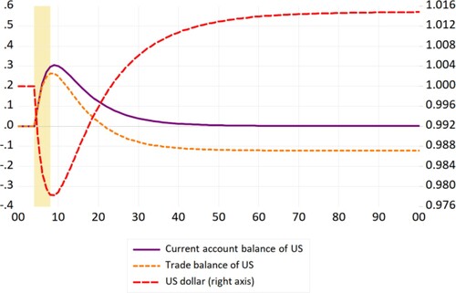
Figure 6. Shock to emulation coefficient.

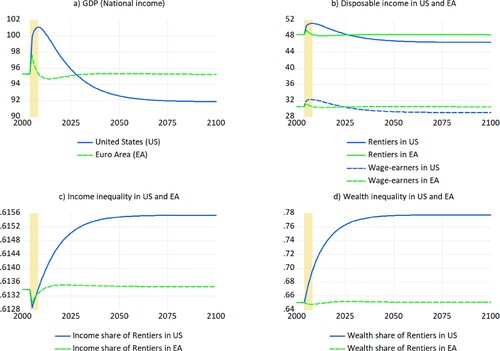
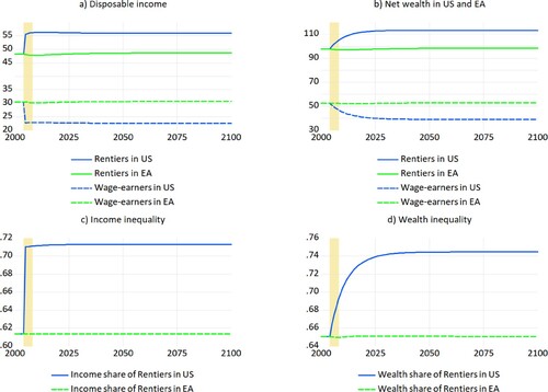
First, despite the initial boom, the new steady state for the US income (or GDP) is lower in the medium run compared with the baseline. Second, both low- and high-income households in the US are affected. Their disposable incomes are lower in the new steady state. This may look quite surprising. Since high-income households own the banks, consumer credit is associated with a redistribution of income from low-income households to high-income households via interest payments. In addition, the initial boom in production drives up sales, hence entrepreneurial profits of US firms (which are distributed to high-income households). Notice that our findings are not due to the lower propensity to consume of high-income households compared with low-income households (see Figure A1 in the Appendix for a multivariate sensitivity analysis). From this perspective, the model differs from the open-economy models that explain the contractionary effects of currency devaluation through income effects, or more precisely through the transfer of ‘real purchasing power toward economic actors with high marginal propensities to save’ (Krugman and Taylor 1978, p. 446). It also differs from post-Keynesian contributions that link currency depreciation with income redistribution from wages to profits. That is how, in wage-led demand regimes, contractionary effects can be generated by exchange rate adjustments (Blecker 2011). Notice that, in standard SFC models, a lower propensity to consume out of income brings about a higher steady-state level of total income due to a higher level of saving and, consequently, a higher level of public expenditure for the service of the government debt held by the private sector. The ‘disappearance’ of the Keynesian ‘paradox of thrift’ has been thoroughly discussed by Godley and Lavoie (2007). In the open economy, this allows shedding light on the effects of exchange rate adjustments that are independent of cross-sector differences in the propensities to consume. Indeed, the explanation is to be found in the interaction between foreign portfolio investments, exchange rates, and income distribution dynamics in the US. Third, both the US and the EA experience a (slight) increase in income inequality.⁷ The greatest and most asymmetrical effect is recorded in the distribution of wealth. While wealth inequality does not change for the EA, a steep increase is recorded in the US. The steady-state percentage of net wealth held by high-income households increases from 65 to 81%. This is the main long-run implication of US low-income households going into debt, thus eroding their net wealth.

Income inequality does not change much because households’ disposable income decreases roughly at the same rate, independently of their social position. By contrast, the net wealth of rich US households decreases mildly, while the net wealth of poor US households plummets, due to debt accumulation.

As already mentioned, the dynamics displayed in Figure 6 are related to the openness of US and EA economies to the international trade of goods and financial assets under a floating exchange rate regime. An increase in (imitative) consumption of US households supports domestic income, hence imports, in the short run. The US trade balance deteriorates, and so does the current account. The US dollar depreciates with respect to the euro. The current account deficit is mirrored by an inflow of foreign capital (from the EA, in our model). The accumulation of foreign debt puts an additional burden on the external position of the US due to the interest payments. The depreciation of the US dollar helps rebalance the US trade balance, hence the current account. An interesting finding here is that the rebalancing process can entail an ‘overshooting’ of the US current account in the long run, which pushes the US dollar above the initial parity (Figure 7).

Figure 7. CAB and US dollar after shock to emulation.

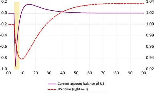
Notice that the current account deficit is completely re-absorbed six periods after the shock. The US dollar stabilises and the trade balance achieves its steady-state level (which may or may not equal zero). However, the stock of private debt accumulated by US households ends up squeezing their consumption. This reduces US imports, exactly when the small recovery in the EA economy is supporting US exports. The outcome is a surplus in the US current account and an appreciation of the US dollar.

The story is not finished yet. The appreciation of the US dollar has two main consequences: first, it reduces the competitiveness of US products, thus re-absorbing the trade balance surplus; second, it causes capital losses for rich US households, which hold euro-denominated assets. These capital losses affect consumption of both high-income households (direct effect) and low-income households (indirect effect, through the imitation channel). This slows down the adjustment process because it depresses imports despite the strength of the US dollar.

Both high- and low-income households in the US are worse off in the long run, that is, when the debt-fuelled boom fades away. In addition, income and wealth distributions are more unequal. This effect is particularly apparent for the stock of wealth. By contrast, EA households are roughly back at the starting point. The fall in exports, due to the long-run contraction of the US economy, is offset by the depreciation of the euro and the capital gains realised on US dollar-denominated financial assets.

Notice that our findings neither depend on the size of the shock nor on coefficient values (see Figure A2 in the Appendix for a multivariable sensitivity test).

5.2. Economic Consequences of (Rising) Inequality

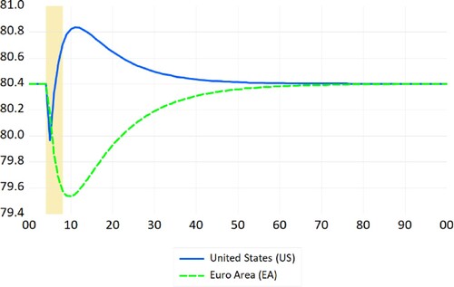
We now focus on the direct effect of a change in the primary distribution of income.⁸ For this purpose, we test the impact of an increase in income inequality in the US economy.⁹ The shock is associated with a short-run recession in the US. The subsequent recovery is not strong enough to bring the economy back to the baseline steady state. Inequality is detrimental to the US economy as a whole in the long run. However, it benefits the Euro Area (in the long run).

The external position of the US and the exchange rate are the keys to understanding the outcome shown in Figure 8. Following the shock, the consumption of low-income households in the US falls. This negative effect is not fully compensated by high-income households’ spending because of their lower propensity to consume. Hence the brief recession in the US. The recession brings about a surplus in both the trade balance and the current account of the US. The EA economy is only slightly hit by the US recession. The US dollar is expected to appreciate as the US trade balance improves. However, the dashed “US dollar” line in Figure 9 shows a depreciation of the US currency. The reason is that higher inequality boosts high-income households’ saving in the US. A share of this saving is used to buy EA financial assets (government bills in our model). The value of capital outflows would exceed the current account surplus if there was no change in the exchange rate.¹⁰ This puts downward pressure on the US dollar.

Figure 8. GDP after shock to wage rate.

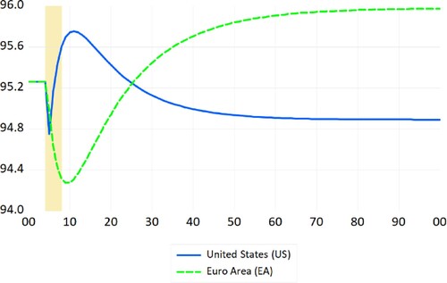
Figure 9. CAB, TB and US dollar after shock to wage rate.

The US dollar depreciation explains why the recession is short-lived. Soon, capital gains on euro-denominated financial assets boost consumption of US households, thus triggering the recovery. In the meantime, the US faces the paradox of a current account surplus coupled with a weak currency. Once again, this is the effect of portfolio investments of US households (while capital losses recorded by EA investors reduce EA imports, despite a stronger currency).

One could infer that a more unequal distribution of income has been beneficial for both the US economy and high-income households in the US. Notice that this result does not depend on differences in the marginal propensities to consume between different sectors of the population, which are usually invoked to explain the contractionary effect of bottom-up redistributions of income and wealth.

The situation reverses when the portfolio adjustment of US households is completed, that is, when there are no more capital outflows to the EA (which offset the US current account surplus). When this happens, the US dollar appreciates, thus slowing down the US economy.

The US dollar is stronger in the new steady state relative to the pre-shock baseline. The large amount of EA financial assets accumulated by US households implies a constant flow of interest payments from the EA. This decreases the demand for euros in the foreign exchange market and sustains the value of the US dollar. This is the reason why the US current account (see Figure 9) is perfectly balanced in the long run despite the permanent trade balance deficit. It is the upward pressure on the US dollar that is responsible for the ‘hard landing’ of the US economy after the middle-term boom.

Notice that US gross national product (GNP, which takes into account the net income earned by residents from overseas investments) is higher than US GDP in the new steady state. The reason is that the trade balance deficit is offset by the surplus of international capital income. However, the steady-state level for US GNP is also lower after the shock because the US dollar appreciation makes the second recession more intense.

One way in which to double-check the narrative above is to test the effect of a change in return rate on EA bills on the US dollar. If the narrative is correct, the lower (higher) the return rate on EA bills, the lower (higher) the amount of interest payments from the EA to the US, the weaker (stronger) must be the US dollar in the long run. If the return rate was nil, there should be no long-term effect of a bottom-up redistribution of income in the US on the dollar exchange rate and therefore on the US economy.

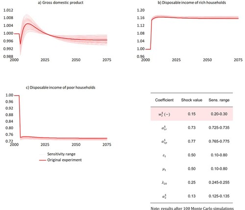
Figure 10 shows that this is exactly what happens in our model. A sensitivity test is provided in Figure A3 in the Appendix, which confirms that results are robust. The only circumstance in which US total income after the shock is higher (relative to its pre-shock value) is when the parameters defining the sensitivity of imports and exports to the exchange rate are doubled (${ϵ}_1$ and ${\mu }_1$ from 0.5–1). This is no surprise. If the adjustment in the current account is quick enough, it keeps US households from accumulating excess foreign assets (thus preventing the over-appreciation of the US dollar).

Figure 10. GDP after shock to wage rate (with interest rates = 0).

Finally, Figure 11 displays the evolution of households’ disposable income, and income and wealth distribution indices, following the shock to the inequality coefficient. Despite the decline in total US income, high-income households in the US are better off at the end of the process, whereas low-income households are worse off. Not only has income inequality increased¹¹ but wealth inequality has significantly grown in the US. By contrast, income and wealth distribution indices in the EA have not been affected, while the total level of income has benefitted from the rise in inequality in the US (we refer again to Figure A3 in the Appendix for a multivariable sensitivity test).

Figure 11. Shock to wage rate.

These dynamics also help us to understand phenomena that took place in recent decades at the world level and are often described as a paradox. On the one hand, we experienced a marked increase in the level of inequality within rich countries. On the other hand, international inequality between countries has decreased when the convergence of per capita income is considered (Darvas 2016). Not only are these conflicting forces actually at work simultaneously but they could even be strictly related, in the sense that the first one could be among the pushing factors behind the second one. The mid-term impact of the Covid-19 pandemic is likely to deploy a similar pattern, as the growing inequality within early-industrialised economies is matched by the reduction of cross-country inequality (mainly due to China catching up with European countries and the US).

6. Evidence from the United States

Despite its simplicity, the model allows replicating fairly well the debt-led boom and bust dynamics that characterised the US crisis of 2007–08. Figure 12 compares the theoretical results produced by the model (under experiment 1) with the available time series for the US economy throughout the crisis.¹²

Figure 12. Shock to emulation coefficient: simulations versus observed series.

Notes: (a) US household debt, percentage of total income, not seasonally-adjusted, source: Federal Reserve Economic Data, 2021; (b) EUR/USD exchange rate, not seasonally-adjusted, source: BIS Statistics Explorer, 2021; (c) Trade Weighted US Dollar Index: Broad, Goods (1997 = 100), not seasonally-adjusted, source: Federal Reserve Economic Data, 2021; (d) US CAB, million USD, seasonally-adjusted, source: Federal Reserve Economic Data, 2021; (e) US trade balance, million USD, seasonally-adjusted, source: Federal Reserve Economic Data, 2021; (f) Inequality of income US, non-wage income share to total income, source: World Inequality Database, 2021; (g) Inequality of Wealth US, net personal wealth of top 1% to total wealth, source: World Inequality database, 2021. Pale dashed lines show simulation results when households are required to pay back a (fixed rate of) their loans after the shock.

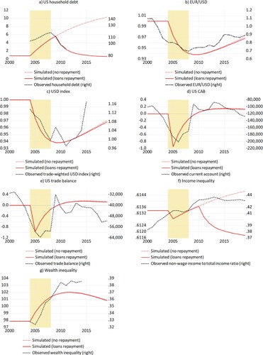
The resemblance of the simulated series with actual data is apparent. The key points can be summarised as follows.

• - The US records an economic boom fuelled by private consumption during the mid-2000s. This goes along with an increase in households’ indebtedness. Their stock of debt is around 103 per cent of GDP at the beginning of 2004 and peaks at approximately 120 per cent in 2008 (Figure 12a).

• - The US dollar constantly depreciates during the boom that precedes the financial crisis of 2007–08 and then rapidly appreciates after it (Figure 12b). Plainly, the appreciation is due to several factors. Arguably, one of the main reasons is the flight-to-safety that usually characterises global crises, which fosters the purchase of dollar-denominated assets.¹³ However, the improvement of the current account balance also plays an important role, which is the one directly captured by our model.

• - Significantly, the US trade balance and current account deteriorate as the US dollar depreciates (Figures 12d and e). This may well appear counter-intuitive, for a weaker currency is usually associated with an improvement in net exports.¹⁴ However, causation works in the opposite direction here: trade balance and current account deficits drive the US dollar downwards. As mentioned, both the current account and the trade balance positions improve post-crisis, mainly due to the fall in imports. These dynamics are also captured by our model.¹⁵

• - Both wealth and income inequality increase during the boom (Figures 12f and g). The crisis tends to crystallise inequality, which is, however, mainly an effect of the previous debt-led boom.

7. Conclusion

We used a two-country macroeconomic model to study the link between inequality and foreign capital flows in the open economy under a floating exchange rate regime. The model is built upon the OPENFLEX model developed by Godley and Lavoie (2007). However, three additional blocks have been added to the original structure: first, each household sector is made up of two different groups, high-income households and low-income households; second, low-income households are characterised by an imitative behaviour, in line with the RIH (Duesenberry 1949; Frank, Levine, and Dijk 2014); third, a simplified financial sector is explicitly modelled. Our experiments show that the emulative consumption of low-income households has a negative impact on the economy in the long run. Both high- and low-income households are affected. In addition, higher inequality is beneficial to the rich but not to the economy as a whole. However, trading partners benefit from higher foreign inequality in the long run. Crucially, these results are only found if households can access credit (to fund extra consumption) and if the economy is open to international trade and capital flows. Moreover, the model replicates reasonably well the empirical evidence from the US crisis of 2007–08, which is arguably the most relevant example of recent debt-led boom and bust dynamics in an advanced economy.

Acknowledgments

We thank the editor and three anonymous referees who provided insightful criticism and suggestions. Of course, all errors remain ours.

Disclosure Statement

No potential conflict of interest was reported by the authors.

Notes

1 Regressions are made using US Census data for the 50 states and the 100 more populous counties in the period between 1990 and 2000, when a steep increase in inequality was recorded.

2 For the sake of simplicity, the interest rate on loans to households is equal to the interest yielded by government bills.

3 Since the model is symmetrical, we omit the equations for the other country, the US.

4 We start from equation (7) because we follow the numbering of the complete list of equations featured in the Appendix.

5 Total gross wealth equals net wealth plus the stock of debt (loans).

6 For this purpose, we change $\mathrm{em}{u}^{\text{€}}$ from 0 to 0.15. Notice that the assumption of country-specific imitation parameters, as proposed by Belabed, Theobald, and van Treeck (2018), can be extended to justify time-specific imitation parameters within the same country.

7 Income (wealth) inequality is calculated as the ratio of the income (wealth) perceived by the top 50 per cent to total income after taxes (wealth).

8 The primary distribution of income is income net of interest payments and other financial incomes.

9 The wage equation coefficient $w_2^{\mathrm{\$}}$ is reset to –0.2. This brings about lower wages for low-income households and higher profits for high-income households.

10 Clearly, this is just a ‘mental experiment’ focusing on (theoretical) intra-period disequilibria before the change in the exchange rate.

11 This comment is actually less trivial than it looks at first sight. It is true that income inequality has been exogenously increased. However, this only relates to the primary distribution of wages, being bank profits and interest rates of bonds related to stocks determined endogenously. Consequently, as in Cardaci and Saraceno (2016), even if the level of inequality is ‘shocked’ exogenously, stocks ‘might allow income distribution to change endogenously’ (p. 19). Tracking the evolution of inequality in disposable incomes makes sense precisely because this second endogenous component is incorporated.

12 Simulated series for the US and the EA are dollars and euros, respectively. However, absolute values of simulated series do not match observed values because the aim of the model is to detect trends and allow for a dynamic comparative analysis, rather than to predict actual levels.

13 Notice that flight-to-safety behaviours can be explicitly reproduced by endogenising the parameters of portfolio equations in our model. However, we chose to ignore this complication as the model is already replicating major stylised facts.

14 This requires the price elasticity of imports and exports to be high enough. For a thorough discussion of this point and a criticism of the standard Marshall–Lerner condition, we refer to Carnevali, Fontana, and Veronese Passarella (2020).

15 The US current account does not become positive, as happens in our simulations. The reason is that the US dollar appreciation was strengthened by the flight-to-safety of foreign capital (see footnote 12). In addition, US exports were also hit by the global crisis.

APPENDIX I

SENSITIVITY ANALYSES

Figure A1. Sensitivity analysis: different combinations of emulation coefficients and propensities to consume.

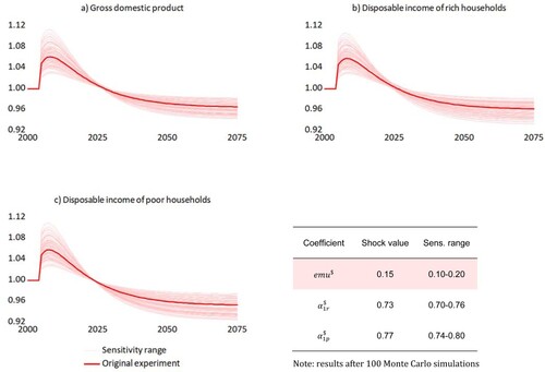
Figure A2. Sensitivity analysis: different combinations of emulation coefficients and other parameters.

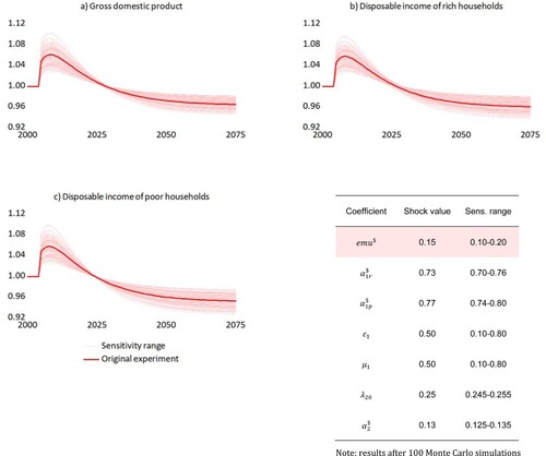
Figure A3. Sensitivity analysis: different combinations of emulation coefficients and other parameters.

APPENDIX II

The complete MODEL

A1. Equations

(1) $Y{D}_r^{\mathrm{\$}}=F_f^{\mathrm{\$}}+F_{\mathrm{bank}}^{\mathrm{\$}}+r_{-1}^{\mathrm{\$}}\cdot B_{\mathrm{\$}s-1}^{\mathrm{\$}}+r_{-1}^{\text{€}}\cdot B_{\text{€}s-1}^{\text{€}}\cdot x{r}^{\text{€}}-T_r^{\mathrm{\$}}$(1) (2) $Y{D}_p^{\mathrm{\$}}=W{B}^{\mathrm{\$}}-r_{-1}^{\mathrm{\$}}\cdot L_d^{\mathrm{\$}}-T_p^{\mathrm{\$}}$(2) (3) $Y{D}_{\mathrm{hsr}}^{\mathrm{\$}}=Y{D}_r^{\mathrm{\$}}+\mathrm{\Delta x}{r}^{\text{€}}\cdot B_{\mathrm{\$}s-1}^{\text{€}}$(3) (4) $\mathrm{\Delta }{V}_r^{\mathrm{\$}}=Y{D}_{\mathrm{hsr}}^{\mathrm{\$}}-C_r^{\mathrm{\$}}$(4) (5) $\mathrm{\Delta }{V}_p^{\mathrm{\$}}=Y{D}_p^{\mathrm{\$}}-C_p^{\mathrm{\$}}+\mathrm{\Delta }{L}_p^{\mathrm{\$}}$(5) (6) $N{W}_p^{\mathrm{\$}}=V_p^{\mathrm{\$}}-L_p^{\mathrm{\$}}$(6) (7) $Y{D}_r^{\text{€}}=F_f^{\text{€}}+F_{\mathrm{bank}}^{\text{€}}+r_{-1}^{\text{€}}\cdot B_{\text{€},s,-1}^{\text{€}}+r_{-1}^{\mathrm{\$}}\cdot B_{\text{€},s,-1}^{\mathrm{\$}}\cdot x{r}^{\mathrm{\$}}-T_r^{\text{€}}$(7) (8) $Y{D}_p^{\text{€}}=W{B}^{\text{€}}-r_{-1}^{\text{€}}\cdot L_d^{\text{€}}-T_p^{\text{€}}$(8) (9) $Y{D}_{\mathrm{hs},r}^{\text{€}}=Y{D}_r^{\text{€}}+\mathrm{\Delta x}{r}^{\mathrm{\$}}\cdot B_{\text{€},s,-1}^{\mathrm{\$}}$(9) (10) $\mathrm{\Delta }{V}_r^{\text{€}}=Y{D}_{\mathrm{hsr}}^{\text{€}}-C_r^{\text{€}}$(10) (11) $\mathrm{\Delta }{V}_p^{\text{€}}=Y{D}_p^{\text{€}}-C_p^{\text{€}}+\mathrm{\Delta }{L}_p^{\text{€}}$(11) (12) $N{W}_p^{\text{€}}=V_p^{\text{€}}-L_p^{\text{€}}$(12) (13) $T^{\mathrm{\$}}={\theta }^{\mathrm{\$}}\cdot \left(F_f^{\mathrm{\$}}+W{B}^{\mathrm{\$}}+r_{-1}^{\mathrm{\$}}\cdot B_{\mathrm{\$}s-1}^{\mathrm{\$}}+r_{-1}^{\text{€}}\cdot B_{\text{€}s-1}^{\text{€}}\cdot x{r}^{\text{€}}+F_{\mathrm{bank}}^{\mathrm{\$}}\right)$(13) (14) $T^{\text{€}}={\theta }^{\text{€}}\cdot \left(F_f^{\text{€}}+W{B}^{\text{€}}+r_{-1}^{\text{€}}\cdot B_{\text{€}s-1}^{\text{€}}+r_{-1}^{\mathrm{\$}}\cdot B_{\text{€}s-1}^{\mathrm{\$}}\cdot x{r}^{\mathrm{\$}}+F_{\mathrm{bank}}^{\mathrm{\$}}\right)$(14) (15) $C_r^{\mathrm{\$}}={\alpha }_{1r}^{\mathrm{\$}}\cdot Y{D}_r^{\mathrm{\$}}\cdot \frac{p_{\mathrm{ex}}^{\mathrm{\$}}}{p^{\mathrm{\$}}}+{\alpha }_2^{\mathrm{\$}}\cdot V_{r-1}^{\mathrm{\$}}$(15) (16) $C_p^{\mathrm{\$}}=\left(1-\mathrm{em}{u}^{\mathrm{\$}}\right)\cdot \left({\alpha }_{1p}^{\mathrm{\$}}\cdot Y{D}_p^{\mathrm{\$}}\cdot {\displaystyle \frac{p_{\mathrm{ex}}^{\mathrm{\$}}}{p^{\mathrm{\$}}}+{\alpha }_2^{\mathrm{\$}}\cdot N{W}_{p-1}^{\mathrm{\$}}}\right)+\mathrm{em}{u}^{\mathrm{\$}}\cdot C_r^{\mathrm{\$}}$(16) (17) $Y^{\mathrm{\$}}=C_r^{\mathrm{\$}}+C_p^{\mathrm{\$}}+G^{\mathrm{\$}}+X^{\mathrm{\$}}-I{M}^{\mathrm{\$}}+I^{\mathrm{\$}}$(17) (18) $F_f^{\mathrm{\$}}=Y^{\mathrm{\$}}-W{B}^{\mathrm{\$}}-r_{-1}^{\mathrm{\$}}\cdot L_f^{\mathrm{\$}}-F_u^{\mathrm{\$}}$(18) (19) $W{B}^{\mathrm{\$}}=W^{\mathrm{\$}}\cdot N_d^{\mathrm{\$}}$(19) (20) $C_r^{\text{€}}={\alpha }_{1r}^{\text{€}}\cdot Y{D}_r^{\text{€}}\cdot {\displaystyle \frac{p_{\mathrm{ex}}^{\text{€}}}{p^{\text{€}}}+{\alpha }_2^{\text{€}}\cdot V_{r-1}^{\text{€}}}$(20) (21) $C_p^{\text{€}}=\left(1-\mathrm{em}{u}^{\text{€}}\right)\cdot \left({\alpha }_{1p}^{\text{€}}\cdot Y{D}_p^{\text{€}}\cdot {\displaystyle \frac{p_{\mathrm{ex}}^{\text{€}}}{p^{\text{€}}}+{\alpha }_2^{\text{€}}\cdot N{W}_{p-1}^{\text{€}}}\right)+\mathrm{em}{u}^{\text{€}}\cdot C_r^{\text{€}}$(21) (22) $Y^{\text{€}}=C_r^{\text{€}}+C_p^{\text{€}}+G^{\text{€}}+X^{\text{€}}-I{M}^{\text{€}}+I^{\text{€}}$(22) (23) $F_f^{\text{€}}=Y^{\text{€}}-W{B}^{\text{€}}-r_{-1}^{\text{€}}\cdot L_f^{\text{€}}-F_u^{\text{€}}$(23) (24) $W{B}^{\text{€}}=W^{\text{€}}\cdot N_d^{\text{€}}$(24) (25) $\log \left(X^{\mathrm{\$}}\right)={ϵ}_0-{ϵ}_1\cdot \log \left(x{r}_{-1}^{\mathrm{\$}}\right)+{ϵ}_2\cdot \log \left(Y^{\text{€}}\right)+{ϵ}_3\cdot \log \left({\displaystyle \frac{p_{\text{€}}^{\mathrm{\$}}}{p^{\mathrm{\$}}}}\right)$(25) (26) $\log \left(I{M}^{\mathrm{\$}}\right)={\mu }_0+{\mu }_1\cdot \log \left(x{r}_{-1}^{\mathrm{\$}}\right)+{\mu }_2\cdot \log \left(Y^{\mathrm{\$}}\right)+{ϵ}_3\cdot \log \left(\frac{p^{\mathrm{\$}}}{p_{\text{€}}^{\mathrm{\$}}}\right)$(26) (27) $X^{\text{€}}=I{M}^{\mathrm{\$}}\cdot x{r}^{\mathrm{\$}}$(27) (28) $I{M}^{\text{€}}=X^{\mathrm{\$}}\cdot x{r}^{\mathrm{\$}}$(28) (29) $B_{\mathrm{\$}d}^{\mathrm{\$}}=V_r^{\mathrm{\$}}\cdot \left({\lambda }_{10}+{\lambda }_{11}\cdot r^{\mathrm{\$}}-{\lambda }_{12}\cdot r^{\text{€}}\right)$(29) (30) $B_{\mathrm{\$}d}^{\text{€}}=V_r^{\mathrm{\$}}\cdot \left({\lambda }_{20}-{\lambda }_{21}\cdot r^{\mathrm{\$}}+{\lambda }_{22}\cdot r^{\text{€}}\right)$(30) (31) $\mathrm{DE}{P}_r^{\mathrm{\$}}=\left(V_r^{\mathrm{\$}}-B_{\mathrm{\$}s}^{\mathrm{\$}}-x{r}^{\text{€}}\cdot B_{\mathrm{\$}s}^{\text{€}}\right)\cdot \mathrm{deps}{h}^{\mathrm{\$}}$(31) (32) $H_{\mathrm{rh}}^{\mathrm{\$}}=V_r^{\mathrm{\$}}-B_{\mathrm{\$}s}^{\mathrm{\$}}-B_{\mathrm{\$}s}^{\text{€}}\cdot x{r}^{\text{€}}-\mathrm{DE}{P}_r^{\mathrm{\$}}$(32) (33) $\mathrm{DE}{P}_p^{\mathrm{\$}}=V_p^{\mathrm{\$}}\cdot \mathrm{deps}{h}^{\mathrm{\$}}$(33) (34) $H_{\mathrm{ph}}^{\mathrm{\$}}=V_p^{\mathrm{\$}}-\mathrm{DE}{P}_p^{\mathrm{\$}}$(34) (35) $H_h^{\mathrm{\$}}=H_{\mathrm{rh}}^{\mathrm{\$}}+H_{\mathrm{ph}}^{\mathrm{\$}}$(35) (36) $B_{\text{€}d}^{\text{€}}=V_r^{\text{€}}\cdot \left({\lambda }_{40}+{\lambda }_{41}\cdot r^{\text{€}}-{\lambda }_{42}\cdot r^{\mathrm{\$}}\right)$(36) (37) $B_{\text{€}d}^{\mathrm{\$}}=V_r^{\text{€}}\cdot \left({\lambda }_{50}-{\lambda }_{51}\cdot r^{\text{€}}+{\lambda }_{52}\cdot r^{\mathrm{\$}}\right)$(37) (38) $\mathrm{DE}{P}_r^{\text{€}}=(V_r^{\text{€}}-B_{\text{€}s}^{\text{€}}-x{r}^{\mathrm{\$}}\cdot B_{\text{€}s}^{\text{€}})\cdot \mathrm{deps}{h}^{\text{€}}$(38) (39) $H_{\mathrm{rh}}^{\text{€}}=V_r^{\text{€}}-B_{\text{€}s}^{\text{€}}-B_{\text{€}s}^{\mathrm{\$}}\cdot x{r}^{\mathrm{\$}}-\mathrm{DE}{P}_r^{\text{€}}$(39) (40) $\mathrm{DE}{P}_p^{\text{€}}=V_p^{\text{€}}\cdot \mathrm{deps}{h}^{\text{€}}$(40) (41) $H_{\mathrm{ph}}^{\text{€}}=V_p^{\text{€}}-\mathrm{DE}{P}_p^{\text{€}}$(41) (42) $H_h^{\text{€}}=H_{\mathrm{rh}}^{\text{€}}+H_{\mathrm{ph}}^{\text{€}}$(42) (43) $B_{\mathrm{\$}s}^{\mathrm{\$}}=B_{\mathrm{\$}d}^{\mathrm{\$}}$(43) (44) $B_{\text{€}s}^{\text{€}}=B_{\text{€}d}^{\text{€}}$(44) (45) $B_{\text{€}s}^{\mathrm{\$}}=B_{\text{€}d}^{\mathrm{\$}}\cdot x{r}^{\text{€}}$(45) (45bis) $B_{\text{€}s}^{\mathrm{\$}}=B_{\mathrm{s}}^{\mathrm{\$}}-B_{\mathrm{\$}s}^{\mathrm{\$}}-B_{\mathrm{cb}\mathrm{\$}s}^{\mathrm{\$}}-B_{\mathrm{bank}}^{\mathrm{\$}}$(45bis) (46) $B_{\mathrm{\$}s}^{\text{€}}=B_{\mathrm{\$}d}^{\text{€}}\cdot x{r}^{\mathrm{\$}}$(46) (47) $\mathrm{DE}{P}_{\mathrm{bank}}^{\mathrm{\$}}=\mathrm{DE}{P}_p^{\mathrm{\$}}+\mathrm{DE}{P}_r^{\mathrm{\$}}$(47) (48) ${\text{β}}_{\mathrm{con}}^{\mathrm{\$}}=1\mathrm{iff}\left(C_p^{\mathrm{\$}}-Y{D}_p^{\mathrm{\$}}\right)>0,\mathrm{otherwise}{\text{β}}_{\mathrm{con}}^{\mathrm{\$}}=0$(48) (49) $\mathrm{\Delta }{L}_h^{\mathrm{\$}}=\left(C_p^{\mathrm{\$}}-Y{D}_p^{\mathrm{\$}}\right)\cdot \left(1-b{o}^{\mathrm{\$}}\right)\cdot {\text{β}}_{\mathrm{con}}^{\mathrm{\$}}-\mathrm{re}{p}^{\mathrm{\$}}\cdot L_{h-1}^{\mathrm{\$}}$(49) (50) $L_s^{\mathrm{\$}}=L_h^{\mathrm{\$}}+L_f^{\mathrm{\$}}$(50) (51) $B_{\mathrm{bnot}}^{\mathrm{\$}}=\mathrm{DE}{P}_{\mathrm{bank}}^{\mathrm{\$}}-L_s^{\mathrm{\$}}$(51) (52) $z^{\mathrm{\$}}=1\mathrm{iff}{B}_{\mathrm{banknot}}^{\mathrm{\$}}>0,\mathrm{otherwise}{z}^{\mathrm{\$}}=0$(52) (53) $B_{\mathrm{bank}}^{\mathrm{\$}}=z^{\mathrm{\$}}\cdot B_{\mathrm{bnot}}^{\mathrm{\$}}$(53) (54) $A_d^{\mathrm{\$}}=-B_{\mathrm{bnot}}^{\mathrm{\$}}\cdot \left(1-z^{\mathrm{\$}}\right)$(54) (55) $A_s^{\mathrm{\$}}=A_d^{\mathrm{\$}}$(55) (56) $F_{\mathrm{bank}}^{\mathrm{\$}}=r_{-1}^{\mathrm{\$}}\cdot B_{\mathrm{bank}-1}^{\mathrm{\$}}+r_{-1}^{\mathrm{\$}}\cdot L_{s-1}^{\mathrm{\$}}$(56) (57) $\mathrm{DE}{P}_{\mathrm{bank}}^{\text{€}}=\mathrm{DE}{P}_p^{\text{€}}+\mathrm{DE}{P}_r^{\text{€}}$(57) (58) ${\text{β}}_{\mathrm{con}}^{\text{€}}=1\mathrm{iff}\left(C_p^{\text{€}}-Y{D}_p^{\text{€}}\right)>0,\mathrm{otherwise}{\text{β}}_{\mathrm{con}}^{\text{€}}=0$(58) (59) $\mathrm{\Delta }{L}_h^{\text{€}}=\left(C_p^{\text{€}}-Y{D}_p^{\text{€}}\right)\cdot \left(1-b{o}^{\text{€}}\right)\cdot {\text{β}}_{\mathrm{con}}^{\text{€}}-\mathrm{re}{p}^{\text{€}}\cdot L_{h-1}^{\text{€}}$(59) (60) $L_s^{\text{€}}=L_h^{\text{€}}+L_f^{\text{€}}$(60) (61) $B_{\mathrm{bnot}}^{\text{€}}=\mathrm{DE}{P}_{\mathrm{bank}}^{\text{€}}-L_s^{\text{€}}$(61) (62) $z^{\text{€}}=1\mathrm{iff}{B}_{\mathrm{banknot}}^{\text{€}}>0,\mathrm{otherwise}{z}^{\text{€}}=0$(62) (63) $B_{\mathrm{bank}}^{\text{€}}=z^{\text{€}}\cdot B_{\mathrm{bnot}}^{\text{€}}$(63) (64) $A_d^{\text{€}}=-B_{\mathrm{bnot}}^{\text{€}}\cdot \left(1-z^{\text{€}}\right)$(64) (65) $A_s^{\text{€}}=A_d^{\text{€}}$(65) (66) $F_{\mathrm{bank}}^{\text{€}}=r_{-1}^{\text{€}}\cdot B_{\mathrm{bank}-1}^{\text{€}}+r_{-1}^{\text{€}}\cdot L_{s-1}^{\text{€}}$(66) (67) $B_{\mathrm{cb}\mathrm{\$}s}^{\mathrm{\$}}=B_s^{\mathrm{\$}}-B_{\text{€}s}^{\mathrm{\$}}-B_{\mathrm{\$}s}^{\mathrm{\$}}-B_{\mathrm{bank}}^{\mathrm{\$}}$(67) (67bis) $B_{\mathrm{cb}\mathrm{\$}s}^{\mathrm{\$}}=H_s^{\mathrm{\$}}-A_s^{\mathrm{\$}}$(67bis) (68) $H_s^{\mathrm{\$}}=B_{\mathrm{cb}\text{€}s}^{\mathrm{\$}}+A_s^{\mathrm{\$}}$(68) (68bis) $H_s^{\mathrm{\$}}=H_h^{\mathrm{\$}}$(68bis) (69) $F_{\mathrm{cb}}^{\mathrm{\$}}=r_{-1}^{\mathrm{\$}}\cdot B_{\mathrm{cb}\mathrm{\$}s-1}^{\mathrm{\$}}$(69) (70) $B_{\mathrm{cb}\text{€}s}^{\text{€}}=B_s^{\text{€}}-B_{\text{€}s}^{\text{€}}-B_{\mathrm{\$}s}^{\text{€}}-B_{\mathrm{bank}}^{\text{€}}$(70) (71) $H_s^{\text{€}}=B_{\mathrm{cb}\text{€}s}^{\text{€}}+A_s^{\text{€}}$(71) (72) $F_{\mathrm{cb}}^{\text{€}}=r_{-1}^{\text{€}}\cdot B_{\mathrm{cb}\text{€}s-1}^{\text{€}}$(72) (73) $\mathrm{\Delta }{B}_s^{\mathrm{\$}}=G^{\mathrm{\$}}-T^{\mathrm{\$}}+r_{-1}^{\mathrm{\$}}\cdot B_{\mathrm{\$}s-1}^{\mathrm{\$}}-F_{\mathrm{cb}}^{\mathrm{\$}}$(73) (74) $\mathrm{\Delta }{B}_s^{\text{€}}=G^{\text{€}}-T^{\text{€}}+r_{-1}^{\text{€}}\cdot B_{\text{€}s-1}^{\text{€}}-F_{\mathrm{cb}}^{\text{€}}$(74) (75) $x{r}^{\text{€}}={\displaystyle \frac{B_{\text{€}s}^{\mathrm{\$}}}{B_{\text{€}d}^{\mathrm{\$}}}}$(75) (75bis) $x{r}^{\text{€}}={\displaystyle \frac{-X^{\mathrm{\$}}+I{M}^{\mathrm{\$}}+r_{-1}^{\mathrm{\$}}\cdot B_{\text{€}s-1}^{\mathrm{\$}}-\mathrm{\Delta }{B}_{\text{€}s}^{\mathrm{\$}}}{r_{-1}^{\text{€}}\cdot B_{\mathrm{\$}s-1}^{\text{€}}-\mathrm{\Delta }{B}_{\mathrm{\$}s}^{\text{€}}}}$(75bis) (76) $x{r}^{\mathrm{\$}}={\displaystyle \frac{1}{x{r}^{\text{€}}}}$(76) (77) $F_u^{\mathrm{\$}}={\delta }^{\mathrm{\$}}\cdot K^{\mathrm{\$}}$(77) (78) $K^{\mathrm{\$}}=K_{-1}^{\mathrm{\$}}\cdot \left(1-{\delta }_{-1}^{\mathrm{\$}}\right)+I^{\mathrm{\$}}$(78) (79) $I^{\mathrm{\$}}={\gamma }^{\mathrm{\$}}\cdot \left(Y^{\mathrm{\$}}\cdot {\kappa }^{\mathrm{\$}}\cdot {\displaystyle \frac{p_{\mathrm{ex}}^{\mathrm{\$}}}{p^{\mathrm{\$}}}-K_{-1}^{\mathrm{\$}}}\right)+{\delta }_{-1}^{\mathrm{\$}}\cdot K_{-1}^{\mathrm{\$}}$(79) (80) $L_f^{\mathrm{\$}}=L_{f-1}^{\mathrm{\$}}+I^{\mathrm{\$}}-F_u^{\mathrm{\$}}$(80) (81) $F_u^{\text{€}}={\delta }^{\text{€}}\cdot K^{\text{€}}$(81) (82) $K^{\text{€}}=K_{-1}^{\text{€}}\cdot \left(1-{\delta }_{-1}^{\text{€}}\right)+I^{\text{€}}$(82) (83) $I^{\text{€}}={\gamma }^{\text{€}}\cdot \left(Y^{\text{€}}\cdot {\kappa }^{\text{€}}\cdot {\displaystyle \frac{p_{\mathrm{ex}}^{\text{€}}}{p^{\text{€}}}-K_{-1}^{\text{€}}}\right)+{\delta }_{-1}^{\text{€}}\cdot K_{-1}^{\text{€}}$(83) (84) $L_f^{\text{€}}=L_{f-1}^{\text{€}}+I^{\text{€}}-F_u^{\text{€}}$(84) (85) $p^{\mathrm{\$}}=\left(1+\mu \right)\cdot \frac{W^{\mathrm{\$}}}{a^{\mathrm{\$}}}$(85) (86) $p^{\text{€}}=\left(1+\mu \right)\cdot {\displaystyle \frac{W^{\text{€}}}{a^{\text{€}}}}$(86) (87) $p_{\mathrm{ex}}^{\mathrm{\$}}=p_{-1}^{\mathrm{\$}}$(87) (88) $p_{\mathrm{ex}}^{\text{€}}=p_{-1}^{\text{€}}$(88) (89) $N_d^{\mathrm{\$}}=\frac{Y^{\mathrm{\$}}}{a^{\mathrm{\$}}}$(89) (90) $N_d^{\text{€}}={\displaystyle \frac{Y^{\text{€}}}{a^{\text{€}}}}$(90) (91) $N_s^{\mathrm{\$}}=N_d^{\mathrm{\$}}$(91) (92) $N_s^{\text{€}}=N_d^{\text{€}}$(92) (93) ${\mathrm{\Omega }}^{\mathrm{\$}}={\frac{\mathrm{WB}}{Y^{\mathrm{\$}}}}^{\mathrm{\$}}$(93) (94) ${\mathrm{\Omega }}^{\text{€}}={\displaystyle {\frac{\mathrm{WB}}{Y^{\text{€}}}}^{\text{€}}}$(94) (95) $\mathrm{LA}{B}^{\mathrm{\$}}=l_0^{\mathrm{\$}}+l_1^{\mathrm{\$}}\cdot \left(N_d^{\mathrm{\$}}-\mathrm{LA}{B}_{-1}^{\mathrm{\$}}\right)$(95) (96) $\mathrm{LA}{B}^{\text{€}}=l_0^{\text{€}}+l_1^{\text{€}}\cdot (N_d^{\text{€}}-\mathrm{LA}{B}_{-1}^{\text{€}}$(96) (97) $U{N}^{\mathrm{\$}}=1-\frac{N_d^{\mathrm{\$}}}{\mathrm{LA}{B}^{\mathrm{\$}}}$(97) (98) $U{N}^{\text{€}}=1-{\displaystyle \frac{N_d^{\text{€}}}{\mathrm{LA}{B}^{\text{€}}}}$(98) (99) $W^{\mathrm{\$}}=\left[1+w_1^{\mathrm{\$}}\cdot \left(U{N}_{-1}^{\mathrm{\$}}-U{N}_n^{\mathrm{\$}}\right)\right]\cdot W_{-1}^{\mathrm{\$}}\cdot \frac{p_{\mathrm{ex}}^{\mathrm{\$}}}{p_{-1}^{\mathrm{\$}}}+w_2^{\mathrm{\$}}$(99) (100) $W^{\text{€}}=\left[1+w_1^{\text{€}}\cdot \left(U{N}_{-1}^{\text{€}}-U{N}_n^{\text{€}}\right)\right]\cdot W_{-1}^{\text{€}}\cdot {\displaystyle \frac{p_{\mathrm{ex}}^{\text{€}}}{p_{-1}^{\text{€}}}+w_2^{\text{€}}}$(100) (101) $p_{\text{€}}^{\mathrm{\$}}=p^{\text{€}}\cdot x{r}^{\text{€}}$(101)

A2. Redundant equations:

(102) $H_h^{\text{€}}=H_s^{\text{€}}$(102) (103) $H_h^{\mathrm{\$}}=H_s^{\text{€}}$(103)

Notes: ‘bis’ equations define the standard Godley and Lavoie (2007)’s exchange rate mechanism. We use an alternative closure of the model based on a simple ‘balance of payments’ approach. The two closures lead to identical results.

A3. Key to symbols and initial values of (lagged) endogenous variables, exogenous variables and parameters. Exogenous variables and parameters are written in bold characters.

Table

Symbol	Description	Value
$A_d^{\text{€}}$	Advances demanded by the EA banking sector to EA central bank	0
$A_d^{\mathrm{\$}}$	Advances demanded by US banking sector to US central bank	0
$A_s^{\text{€}}$	Advances supply by EA central bank	0
$A_s^{\mathrm{\$}}$	Advances supply by US central bank	0
$B_{\mathrm{cb}\text{€}s}^{\text{€}}$	EA bills held by EA central bank	0
$B_{\mathrm{cb}\mathrm{\$s}}^{\mathrm{\$}}$	US bills held by US central bank	0
$B_{\text{€}d}^{\text{€}}$	Demand for EA bills by EA rich households	0
$B_{\text{€}d}^{\mathrm{\$}}$	Demand for US bills by EA rich households	0
$B_{\mathrm{\$}d}^{\mathrm{\$}}$	Demand for US bills by US rich households	0
$B_{\mathrm{\$}d}^{\text{€}}$	Demand for EA bills by US rich households	0
$B_{\text{€}s}^{\text{€}}$	EA bills held by EA rich households (bills supply)	0
$B_{\text{€}s}^{\mathrm{\$}}$	US bills held by EA rich households (bills supply)	0
$B_{\mathrm{\$}s}^{\mathrm{\$}}$	US bills held by US rich households (bills supply)	0
$B_{\mathrm{\$}s}^{\text{€}}$	EA bills held by US rich households (bills supply)	0
$B_{\mathrm{bnot}}^{\text{€}}$	Notional level of domestic bills held by the EA banking sector	0
$B_{\mathrm{bnot}}^{\mathrm{\$}}$	Notional level of domestic bills held by the US banking sector	0
$B_s^{\text{€}}$	EA public debt (total EA bills issued)	0
$B_s^{\mathrm{\$}}$	US public debt (total US bills issued)	0
$B_{\mathrm{bank}}^{\text{€}}$	Actual level of domestic bills held by the EA banking sector	0
$B_{\mathrm{bank}}^{\mathrm{\$}}$	Actual level of domestic bills held by the US banking sector	0
$C_r^{\text{€}}$	Value of consumption of EA rich households	-
$C_p^{\text{€}}$	Value of consumption of EA poor households	-
$C_r^{\mathrm{\$}}$	Value of consumption of US rich households	-
$C_p^{\mathrm{\$}}$	Value of consumption of US poor households	-
$\mathrm{DE}{P}_r^{\text{€}}$	Demand of bank deposits by EA rich households	0
$\mathrm{DE}{P}_p^{\text{€}}$	Demand of bank deposits by EA poor households	0
$\mathrm{DE}{P}_r^{\mathrm{\$}}$	Demand of bank deposits by US rich households	0
$\mathrm{DE}{P}_p^{\mathrm{\$}}$	Demand of bank deposits by US poor households	0
$\mathrm{DE}{P}_{\mathrm{bank}}^{\text{€}}$	Total level of deposits in the EA	0
$\mathrm{DE}{P}_{\mathrm{bank}}^{\mathrm{\$}}$	Total level of deposits in the US	0
$F_{\mathrm{bank}}^{\text{€}}$	Profits of the EA banking sector	-
$F_{\mathrm{bank}}^{\mathrm{\$}}$	Profits of the US banking sector	-
$F_{\mathrm{cb}}^{\text{€}}$	EA Central Bank’s profits	-
$F_{\mathrm{cb}}^{\mathrm{\$}}$	US Central Bank’s profits	-
${\mathit{G}}^{\text{€}}$	Initial value of government spending in the EA	16
${\mathit{G}}^{\mathrm{\$}}$	Initial value of government spending in the US	16
$g_{\mathrm{con}}^{\text{€}}$	Borrowing ‘parameter’ of EA poor households	-
$g_{\mathrm{con}}^{\mathrm{\$}}$	Borrowing ‘parameter’ of US poor households	-
$H_{\mathrm{rh}}^{\text{€}}$	Cash held by EA rich households	0
$H_{\mathrm{ph}}^{\text{€}}$	Cash held by EA poor households	0
$H_{\mathrm{rh}}^{\mathrm{\$}}$	Cash held by US rich households	0
$H_{\mathrm{ph}}^{\mathrm{\$}}$	Cash held by US poor households	0
$H_h^{\text{€}}$	Total cash held by EA households	0
$H_h^{\mathrm{\$}}$	Total cash held by US households	0
$H_s^{\text{€}}$	EA money supply	0
$H_s^{\mathrm{\$}}$	US money supply	0
$I{M}^{\text{€}}$	EA imports	-
$I{M}^{\mathrm{\$}}$	US imports	-
$L_p^{\text{€}}$	Demand for loans by EA poor households	0
$L_d^{\mathrm{\$}}$	Demand for loans by US poor households	0
$L_s^{\text{€}}$	Supply of loans by EA banks	0
$L_s^{\mathrm{\$}}$	Supply of loans by US banks	0
$N{W}_p^{\text{€}}$	EA poor households’ net private wealth	0
$N{W}_p^{\mathrm{\$}}$	US poor households’ net private wealth	0
$T^{\text{€}}$	Taxes paid by EA households	-
$T^{\mathrm{\$}}$	Taxes paid by US households	-
$V_r^{\mathrm{\$}}$	US rich households’ private wealth	0
$V_p^{\mathrm{\$}}$	US poor households’ gross private wealth	0
$V_r^{\text{€}}$	EA rich households’ private wealth	0
$V_p^{\text{€}}$	EA poor households’ gross private wealth	0
a$X^{\text{€}}$	EA exports	-
$X^{\mathrm{\$}}$	US exports	-
$Y^{\text{€}}$	EA GDP	-
$Y^{\mathrm{\$}}$	US GDP	-
$Y{D}_r^{\text{€}}$	Regular diosable income EA rich households	-
$Y{D}_p^{\text{€}}$	Regular disposable income EA poor households	-
$Y{D}_r^{\mathrm{\$}}$	Regular disposable income US rich households	-
$Y{D}_p^{\mathrm{\$}}$	Regular disposable income US poor households	-
$Y{D}_{\mathrm{hsr}}^{\text{€}}$	EA rich households Haig-Simons disposable income	-
$Y{D}_{\mathrm{hsr}}^{\mathrm{\$}}$	US rich households Haig-Simons disposable income	-
$z^{\text{€}}$	Trigger for notional EA bills bought by EA bank
$z^{\mathrm{\$}}$	Trigger for notional US bills bought by US bank
${\mathit{a}}^{\text{€}}$	Average labour productivity in the EA	2
${\mathit{a}}^{\mathrm{\$}}$	Average labour productivity in the EA	2
$\mathit{b}{\mathit{o}}^{\text{€}}$	Share of borrowed money out of excessive consumption in the EA	0.5
$\mathit{b}{\mathit{o}}^{\mathrm{\$}}$	Share of borrowed money out of excessive consumption in the US	0.5
$\mathit{deps}{\mathit{h}}^{\text{€}}$	Percentage of money held as deposits in the EA	0.7
$\mathit{deps}{\mathit{h}}^{\mathrm{\$}}$	Percentage of money held as deposits in the US	0.7
$\mathit{em}{\mathit{u}}^{\text{€}}$	Emulation parameter in the EA	0
$\mathit{em}{\mathit{u}}^{\mathrm{\$}}$	Emulation parameter in the US	0
${\mathit{k}}^{\text{€}}$	Desired capital to output stock in the EA	0.1
${\mathit{k}}^{\mathrm{\$}}$	Desired capital to output stock in the US	0.1
${\mathit{l}}_0^{\text{€}}$	Coefficient of EA labour force equation (autonomous component)	50
${\mathit{l}}_0^{\mathrm{\$}}$	Coefficient of US labour force equation (autonomous component)	50
${\mathit{l}}_1^{\text{€}}$	Coefficient of EA labour force equation (dependent component)	0.1
${\mathit{l}}_1^{\mathrm{\$}}$	Coefficient of US labour force equation (dependent component)	0.1
$p^{\text{€}}$	Price level in the EA	1
$p^{\mathrm{\$}}$	Price level in the US	1
$p_{\mathrm{ex}}^{\text{€}}$	Expected Price level in the EA	1
$p_{\mathrm{ex}}^{\mathrm{\$}}$	Expected Price level in the US	1
${\mathit{r}}^{\text{€}}$	Interest rate on EA bills	0.03
$\mathit{r}$	Interest rate on US bills	0.03
$\mathit{re}{\mathit{p}}^{\text{€}}$	Repayment rate of households’ loans in the EA	0
$\mathit{re}{\mathit{p}}^{\mathrm{\$}}$	Repayment rate of households’ loans in the US	0
$U{N}^{\text{€}}$	Actual unemployment rate in the EA (initial value)	0
$U{N}^{\mathrm{\$}}$	Actual unemployment rate in the US (initial value)	0
${\mathit{U}N}_n^{\text{€}}$	Normal rate of unemployment in the EA	0
${\mathit{U}N}_n^{\mathrm{\$}}$	Normal rate of unemployment in the US	0
$W^{\text{€}}$	Money wage rate in the EA	1
$W^{\mathrm{\$}}$	Money wage rate in the EA	1
${\mathit{w}}_1^{\text{€}}$	First coefficient in EA wage equation (sensitivity to unemployment)	0
${\mathit{w}}_1^{\mathrm{\$}}$	First coefficient in US wage equation (sensitivity to unemployment)	0
${\mathit{w}}_2^{\text{€}}$	Second coefficient in EU wage equation (shock)	0
${\mathit{w}}_2^{\mathrm{\$}}$	Second coefficient in US wage equation (shock)	0
$x{r}^{\text{€}}$	EUR to USD exchange rate	1
$x{r}^{\mathrm{\$}}$	USD to EUR exchange rate	1
${\mathit{\alpha }}_{1\mathit{r}}^{\text{€}}$	Propensity to consume out of disposable income of EA high-income households	0.73
${\mathit{\alpha }}_{1\mathit{p}}^{\text{€}}$	Propensity to consume out of disposable income of EA low-income households	0.77
${\mathit{\alpha }}_{1\mathit{r}}^{\mathrm{\$}}$	Propensity to consume out of disposable income of US high-income households	0.73
${\mathit{\alpha }}_{1\mathit{p}}^{\mathrm{\$}}$	Propensity to consume out of disposable income of US low-income households	0.77
${\mathit{\alpha }}_2^{\text{€}}$	Propensity to consume out of net wealth of EA households	0.13333
${\mathit{\alpha }}_2^{\mathrm{\$}}$	Propensity to consume out of net wealth of US households	0.13333
${\mathit{\gamma }}^{\text{€}}$	Speed of adjustment of capital to desired level in the EA	0.15
${\mathit{\gamma }}^{\mathrm{\$}}$	Speed of adjustment of capital to desired level in the US	0.15
${\mathit{ϵ}}_0$	US Real exports constant	-2.1
${\mathit{ϵ}}_1$	Exchange rate elasticity of US real exports	0.5
${\mathit{ϵ}}_2$	Income elasticity of US real exports	1.228
${\mathit{ϵ}}_3$	Relative price elasticity of US real exports	0.1
${\mathit{\theta }}^{\text{€}}$	Tax rate in the EA	0.2
${\mathit{\theta }}^{\mathrm{\$}}$	Tax rate in the US	0.2
${\lambda }_{10}$	First parameter of demand for US bills in the US	0.7
${\lambda }_{11}$	Second parameter of demand for US bills in the US	5
${\lambda }_{12}$	Third parameter of demand for US bills in the US	5
${\lambda }_{20}$	First parameter of demand for EA bills in the US	0.25
${\lambda }_{21}$	Second parameter of demand for EA bills in the US	5
${\lambda }_{22}$	Third parameter of demand for EA bills in the US	5
${\lambda }_{40}$	First parameter of demand for EA bills in the EA	0.7
${\lambda }_{41}$	Second parameter of demand for EA bills in the EA	5
${\lambda }_{42}$	Third parameter of demand for EA bills in the EA	5
${\lambda }_{50}$	First parameter of demand for US bills in the EA	0.25
${\lambda }_{51}$	Second parameter of demand for US bills in the EA	5
${\lambda }_{52}$	Third parameter of demand for US bills in the EA	5
${\mathit{\mu }}_0$	US Real imports constant	-2.1
${\mathit{\mu }}_1$	Exchange rate elasticity of US real imports	0.5
${\mathit{\mu }}_2$	Income elasticity of US real imports	1.228
${\mathit{\mu }}_3$	Relative price elasticity of US real imports	0.1
${\mathit{\delta }}^{\text{€}}$	Capital depreciation rate in the EA	0.5
${\mathit{\delta }}^{\mathrm{\$}}$	Capital depreciation rate in the US	0.5
${\mathit{\rho }}^{\text{€}}$	Min. percentage of low-income households’ loans to disposable income in the EA	0
${\mathit{\rho }}^{\mathrm{\$}}$	Min. percentage of low-income households’ loans to disposable income in the US	0

References

- Abiad, A., N. Oomes, and K. Ueda. 2008. ‘The Quality Effect: Does Financial Liberalization Improve the Allocation of Capital?’ Journal of Development Economics 87 (2): 270–282.
- Aït-Youce, C. 2019. ‘How Index Investment Impacts Commodities: A Story About the Financialisation of Agricultural Commodities.’ Economic Modelling 80: 23–33.
- Behringer, J., and T. van Treeck. 2019. ‘Income Distribution and Growth Models: A Sectoral Balances Approach.’ Politics & Society 47 (3): 303–332.
- Belabed, C. A., T. Theobald, and T. van Treeck. 2018. ‘Income Distribution and Current Account Imbalances.’ Cambridge Journal of Economics 42 (1): 47–94.
- Bhaduri, A. 2011. ‘A Contribution to the Theory of Financial Fragility and Crisis.’ Cambridge Journal of Economics 35 (6): 995–1014.
- Blecker, R. A. 2011. ‘Open Economy Models of Distribution and Growth.’ In A Modern Guide to Keynesian Macroeconomics and Economic Policies, edited by E. Hein, and E. Stockhammer, 215–239. Cheltenham, UK: Edward Elgar Publishing.
- Botta, A., E. Caverzasi, A. Russo, M. Gallegati, and J. E. Stiglitz. 2021. ‘Inequality and Finance in a Rent Economy.’ Journal of Economic Behavior & Organization 183: 998–1029.
- Bottan, N., B. Hoffmann, and D. Vera-Cossio. 2020. ‘The unequal impact of the coronavirus pandemic: Evidence from seventeen developing countries’. IDP Working Papers Series 15 (10). Washington (D.C., USA): Inter-American Development Bank.
- Bowles, S., and Y. Park. 2005. ‘. ‘Emulation, Inequality, and Work Hours: Was Thorsten Veblen Right?’ ‘ The Economic Journal 115 (507): F397–F412.
- Cardaci, A., and F. Saraceno. 2016. ‘Inequality, Financialisation and Credit Booms: a Model of Two Crises.’ SEP Working Papers 2016/2. Rome (Italy): LUISS School of European Political Economy.
- Carnevali, E. 2021. ‘A New, Simple SFC Open Economy Framework.’ Review of Political Economy. Article, doi:10.1080/09538259.2021.1899518.
- Carnevali, E., M. Deleidi, R. Pariboni, and M. Veronese Passarella. 2021. ‘Cross-Border Financial Flows and Global Warming In a Two-Area Ecological SFC Model.’ Socio-Economic Planning Sciences 75.
- Carnevali, E., G. Fontana, and M. Veronese Passarella. 2020. ‘Assessing the Marshall-Lerner Condition Within a Stock-Flow Consistent Model.’ Cambridge Journal of Economics 44 (4): 891–918.
- Christen, M., and R. M. Morgan. 2005. ‘Keeping up with the Joneses: Analyzing the Effect of Income Inequality on Consumer Borrowing.’ Quantitative Marketing and Economics 3 (2): 145–173.
- Cynamon, B. Z., and S. M. Fazzari. 2013. ‘Inequality and Household Finance during the Consumer Age.’ Working Paper 752. Annandale-on-Hudson (New York, USA): Levy Economics Institute of Bard College.
- Dabla-Norris, E., K. Kochhar, F. Ricka, N. Suphaphiphat, and E. Tsounta. 2015. ‘Causes and consequences of income inequality: a global perspective.’ IMF Staff Discussion Note 15/13. Washington (D.C., USA): International Monetary Fund.
- Darvas, Z. 2016. ‘Some are more equal than others: new estimates of global and regional inequality.’ Bruegel Working Paper 2016/08. Brussels (Belgium): Bruegel. Available from: http://bruegel.org/2016/11/some-are-more-equal-than-others-new-estimates-of-global-and-regional-inequality/.
- de Haan, J., and J. E. Sturm. 2017. ‘Finance and Income Inequality: A Review and new Evidence.’ European Journal of Political Economy 50 (C): 171–195.
- Denk, O., and B. Cournede. 2015. ‘Finance and income inequality in OECD countries.’ OECD Economics Department Working Papers 1224. Paris: OECD Publishing.
- Detzer, D. 2018. ‘Inequality, Emulation and Debt: The Occurrence of Different Growth Regimes in the age of Financialisation in a Stock-Flow Consistent Model.’ Journal of Post Keynesian Economics 41 (2): 284–315.
- Dodig, N., and E. Hein. 2015. ‘Finance-dominated Capitalism, Distribution, Growth and Crises – Long-run Tendencies.’ In The Demise of Finance-Dominated Capitalism: Explaining the Financial and Economic Crises, edited by E. Hein, D. Detzer, and N. Dodig. Cheltenham (UK): Edward Elgar.
- D’Orazio, P. 2019. ‘Income Inequality, Consumer Debt, and Prudential Regulation: An Agent-Based Approach to Study the Emergence of Crises and Financial Instability.’ Economic Modelling 82: 308–331.
- Dosi, G., G. Fagiolo, M. Napoletano, and A. Roventini. 2013. ‘Income Distribution, Credit and Fiscal Policies in Anagent-Based Keynesian Model.’ Journal of Economic Dynamics and Control 37 (8): 1598–1625.
- Douglas, M., and B. Isherwood. 1978. The World of Goods. New York (USA): Basic Books.
- Duesenberry, J. S. 1949. Income, Saving and the Theory of Consumer Behaviour. Cambridge (Massachusetts, USA): Harvard University Press.
- Dünhaupt, P. 2017. ‘Determinants of Labour’s Income Share in the era of Financialisation.’.’ Cambridge Journal of Economics 41 (1): 283–306.
- Epstein, G. 2019. The Political Economy of Central Banking. Cheltenham (UK): Edward Elgar Publishing, pp. 380-406.
- Fitoussi, J. P., and F. Saraceno. 2010. ‘Europe: How Deep is the Crisis? Policy Responses and Structural Factors Behind Diverging Performances.’ Journal of Globalization and Development 1 (1): 1–19.
- Frank, R. H. 1985. Choosing the Right Pond: Human Behavior and the Quest for Status. Oxford (UK): Oxford University Press.
- Frank, R. H., A. S. Levine, and O. Dijk. 2014. ‘Expenditure Cascades.’ Review of Behavioral Economics 1 (1–2): 55–73.
- Friedman, M. 1957. A Theory of the Consumption Function. Princeton (New Jersey, USA): Princeton University Press.
- Gaertner, W. 1974. ‘A Dynamic Model of Interdependent Consumer Behavior.’ Zeitschrift für Nationalökonomie/Journal of Economics H 3/4: 327–344.
- Goda, T., and P. Lysandrou. 2014. ‘The Contribution of Wealth Concentration to the Subprime Crisis: A Quantitative Estimation.’ Cambridge Journal of Economics 38 (2): 301–327.
- Godechot, O. 2016. ‘Financialisation Is Marketization! A Study of the Respective Impacts of Various Dimensions of Financialisation on the Increase in Global Inequality.’ Sociological Science 3: 395–519.
- Godley, W. 1996. ‘Money, Finance and National Income Determination: An Integrated Approach.’ Levy Institute Working Paper 167.
- Godley, W., and M. Lavoie. 2007. Monetary Economics: An Integrated Approach to Credit, Money, Income, Production and Wealth. London: Palgrave MacMillan.
- Hayakawa, H., and Y. Venieris. 1977. ‘Consumer Interdependence via Reference Groups.’ Journal of Political Economy 85 (3): 599–615.
- Hein, E. 2015. ‘Finance Dominated Capitalism and Re-Distribution of Income: A Kaleckian Perspective.’ Cambridge Journal of Economics 39 (3): 907–934.
- Hein, E., and N. Dodig. 2015. ‘Finance-dominated Capitalism, Distribution, Growth and Crisis–Long-run Tendencies.’ In The Demise of Finance-Dominated Capitalism, edited by E. Hein, D. Detzer, and N. Dodig, 54–11. Cheltenham (UK): Edward Elgar Publishing.
- Hein, E., P. Dünhaupt, A. Alfageme, and M. Kulesza. 2018. ‘A Kaleckian Perspective on Financialisation and Distribution in Three Main Eurozone Countries Before and After the Crisis: France, Germany and Spain.’ Review of Political Economy 30 (1): 41–71.
- Jauch, S., and S. Watzka. 2012. ‘Financial development and income inequality: a panel data approach.’ CESifo Working Papers 3687. Munich (Germany): CESifo.
- Jaumotte, F., S. Lall, and C. Papageorgiou. 2013. ‘. ‘Rising Income Inequality: Technology, or Trade and Financial Globalization?’ ‘ IMF Economic Review 61 (2): 271–309.
- Jaumotte, F., and C. Osorio Buitron. 2015. ‘Inequality and labor market institutions.’ IMF Staff Discussion Note 15/14. Washington (D.C., USA): International Monetary Fund.
- Kapeller, J., and B. Schutz. 2014. ‘Debt, Boom, Bust: A Theory of Minsky-Veblen Cycles.’ Journal of Post Keynesian Economics 36 (4): 781–814.
- Krelle, W. 1972. ‘Dynamics of the Utility Function.’ Zeitschrift fur Nationalekonomie 32: 59–70.
- Krippner, G. R. 2005. ‘The Financialization of the American Economy.’ Socio-economic Review 3 (2): 173–208.
- Krugman, P., and L. Taylor. 1978. ‘Contractionary Effects of Devaluation.’ Journal of International Economics 8 (3): 445–456.
- Kumhof, M., M. Lebarz, M. Ranciere, M. Richter, and M. Throckmorton. 2012. ‘Income inequality and current account imbalances.’ IMF Working Papers, No 2012/008.
- Kumhof, M., R. Ranciere, and P. Winant. 2015. ‘Inequality, Leverage and Crises.’ American Economic Review 105 (3): 1217–1245.
- Lavoie, M. 2015. Post-Keynesian Economics. New Foundations. Cheltenham (UK): Edward Elgar.
- Li, J., and H. Yu. 2014. ‘Income Inequality and Financial Reform in Asia: The Role of Human Capital.’ Applied Economics 46 (24): 2920–2935.
- Lysandrou, P. 2011. ‘Global Inequality, Wealth Concentration and the Subprime Crisis: A Marxian Commodity Theory Analysis.’ Development and Change 42 (1): 183–208.
- Modigliani, F. 1986. ‘Life Cycle, Individual Thrift, and the Wealth of Nations.’ American Economic Review 76 (3): 297–313.
- Nassif-Pires, L., L. de Lima Xavier, T. Masterson, M. Nikiforos, and F. Rios-Avila. 2020. ‘Pandemic of inequality.’ Public Policy Brief No. 149. Annandale-on-Hudson (New York, USA): Levy Economics Institute.
- Ostvik-White, B. 2003. ‘Income Inequality and Median House Prices in 200 School Districts’. Cornell University Institute of Public Policy Masters Thesis, Ithaca, New York (USA).
- Ouyanga, R., and X. Zhang. 2020. ‘Financialisation of Agricultural Commodities: Evidence from China.’ Economic Modelling 85: 381–389.
- Perry, B. L., B. Aronson, and B. A. Pescosolido. 2021. ‘Pandemic Precarity: COVID-19 is Exposing and Exacerbating Inequalities in the American Heartland.’ Proceedings of the National Academy of Sciences 118 (8).
- Pollak, R. A. 1976. ‘Interdependent Preferences.’ American Economic Review 66 (3): 309–320.
- Qureshi, Z. 2020. ‘Tackling the Inequality Pandemic: Is There a Cure?’ In Reimagining the Global Economy: Building Back Better, edited by B. S. Coulibaly, K. Derviş, H. Kharas, and Z. Qureshi. Washington (DC, US): Brookings Institution.
- Rajan, R. G. 2010. Fault Lines: How Hidden Fractures Still Threaten the World Economy. Princeton (New Jersey, USA): Princeton University Press.
- Russo, A., L. Riccetti, and M. Gallegati. 2016. ‘Increasing Inequality, Consumer Credit and Financial Fragility in an Agent Based Macroeconomic Model.’ Journal of Evolutionary Economics 26 (1): 25–47.
- Stockhammer, E. 2010. ‘Financialization and the Global Economy.’ Political Economy Research Institute Working Paper 242 (40): 1–17.
- Stockhammer, E. 2015. ‘Rising Inequality as a Cause of the Present Crisis.’ Cambridge Journal of Economics 39 (3): 935–958.
- Tobin, J. 1969. ‘A General Equilibrium Approach to Monetary Theory.’ Journal of Money, Credit and Banking 1 (1): 15–29.
- Van Arnum, B. M., and M. I. Naples. 2013. ‘Financialisation and Income Inequality in the United States, 1967–2010.’ The American Journal of Economics and Sociology 72 (5): 1158–1182.
- van Treeck, T. 2014. ‘Did Inequality Cause the US Financial Crisis?’ Journal of Economic Surveys 28 (3): 421–448.
- Veblen, T. 1899. The Theory of the Leisure Class. 1994 Edition. New York (USA): Dover Publications.