The Distributive Monetary Analysis of a (un)Sustainable Economy

ABSTRACT

This article is a post-Keynesian stock flow consistent (PK-SFC) model that analyses the dynamics of an economy characterised by several — often individually studied — features of PK-SFC studies together with some innovative aspects. In particular, we investigate the income and wealth distribution between two social classes, capitalists and workers, after a period of a crisis subject to different policy scenarios. Non-financial firms but also government can undertake investments decisions and both accumulate capital. Finally, we consider the workers' and capitalists' consumption behaviour that contributes to produce (un)sustainable paths. Our model is built upon Bibi (2020, 2021) within an endogenous money framework and is calibrated using available data for major advanced economies. Simulations are conducted to question the different government fiscal policies to reduce unemployment boosting the economic activity, to obtain a more equitable distribution between social classes while obtaining those goals in a sustainable way.

KEYWORDS:

• Kalecki
• post-Keynesian economics
• distribution
• endogenous money
• sustainability

JEL CLASSIFICATIONS:

• E12
• E32
• E51
• E62

1. Introduction

In the years after the 2007 crisis, the recovery and distribution issues revamped interest both in economic theories and political discussions. Together with these, particular attention was paid to the ecological problems associated with the ambitious, but nonetheless necessary, objective of achieving the first two goals in an ecologically sustainable way.

Despite many contributions focused on some of the previous topics, few of them tried to tackle them all in a comprehensive way and considering one of the most important breakthroughs in recent decades, namely, the rediscovery of the endogenous money phenomena. Here, we argue that the endogenous money feature is precisely the essential fil rouge to better understand and connect those three importantly related aspects.

Our work is strongly based on Sawyer (2010), Arestis and Sawyer (2005), Zambelli (2007, 2014), and Bibi (2020, 2021). It is also inspired by Sawyer and Passarella Veronese (2017) and Fontana and Sawyer (2016), who examined environmental aspects within a monetary circuit model, and Dafermos et al. (2017), who integrated thoroughly monetary and physical variables in a coherent ecological stock-flow consistent (SFC) macroeconomic model. The basis of endogenous money and the structure of the economy in what has been known as the post-Keynesian stock-flow consistent approach relies mainly on the work of Graziani (2003), Godley and Lavoie (2007), Fontana and Setterfield (2009), and Rochon et al. (2020).

The structure of our model is an extension of Bibi (2021) but also borrows some key features from Godley and Lavoie (2007). In particular, even if the model described in Godley and Lavoie’s (2007) Chapter 11 is a growth model, our scenario differs from that since it considers a stationary level of output as a starting point but still retains the possibility of capacity output growth. We do that mainly to highlight a more immediate contrast between the policy scenarios simulations and implications contained here and those of Bibi (2021) where capacity output growth is not allowed. In line with Bibi, we take into account that production takes time and that banks create credit money and consider the lack of market clearing conditions. The mismatching between aggregate demand and aggregate production in consumption goods creates inventories.

Different features characterize our model and also distinguish it from Bibi.

• First, households comprise two social groups: workers and capitalists. These households differ not only in terms of their consumption behaviour but also in terms of their initial endowment, of the different conditions of loan repayment required by banks and in terms of how they can use their financeable wealth.

• Second, we consider the a-synchronized Kaleckian investment production process. In line with that, we consider the three different investment stages proposed by Kalecki himself (1971) and developed by Zambelli (2014) and borrowed by Bibi (2021).

• Third, we consider the investments and capital held by both non-financial firms and the government; this distinction is relevant because we want to explore how different drivers of investment can affect the formation of capital and the economic and ecological sustainability of our economy.

• Fourth, and finally, we consider the ecological impacts of workers’ and capitalists’ consumption processes. In particular, their dissimilar consumption level — based on different incomes and wealth — is assumed to have different impacts on the ecological balance and resources needed to obtain the consumption goods required. This seems in line with the conclusions of most studies about environmental pressure related to levels of income (Mackenzie et al. 2008). It is important to highlight here that our work is based on intuition regarding the impact of consumption on ecological variables. Dafermos et al. (2017) consider ecosystem-related variables to a much greater degree; for example, they differentiate between conventional and green investment and discuss how the degradation of ecosystem services has feedback effects on the economy.

This article proceeds as follows. Section Two describes the overall model through its balance sheet and transaction flow matrices. Section Three provides a sketch of the model and underlines the main behavioural rules of its actors. Section Four presents the main simulations based on our key question: how does the government manoeuvre to achieve an economic, social and ecologically sustainable recovery. Section Five offers conclusions.

2. Balance Sheet and Transaction-Flow Matrix

Following Kaleckian features and Bibi (2020, 2021), we describe an economy characterized by two different types of socioeconomic class, namely, workers’ and capitalists’ households. They are different because of their consumption capacity, which is linked to their different purchasing power resulting from both the wealth they are endowed with and the different loan repayment conditions required of them by commercial banks. Finally, even if production firms are described as a separate sector in the economy, these are legally owned by capitalists’ households while workers’ households have no claim on firms beyond the wages they receive from them in return for their labour.

Workers’ and capitalists’ households are allowed to take loans from commercial banks (hereafter, CBs) and they have access to cash and deposits. Workers maintain their wealth in the form of deposits while capitalists maintain their wealth also in the form of bills and long-term bonds. Capitalists are the owners of both financial and non-financial firms and therefore they hold bank funds (OFs), too. In our economy, production firms own both fixed capital and inventories and they are allowed to take loans to finance their productive activity.

The government is supposed to own capital, reflected, for example, in the value of transport and educational infrastructure, while emitting bills and bonds. The country central bank (CCB¹) holds part of the bills emitted by the government and emits cash (H). CBs make loans to firms and households while having treasury bills $\left(B_b\right)$ and cash balances $\left(H_b\right)$. The net worth of the CBs calculated as the difference between assets and liabilities constitutes their own funds ($O{F}_b$) and is also reflected in the balance sheets of their owners, the capitalists (see Table A1).

The transaction-flow matrix (hereafter, TFM) describes how the flows of different sectors of the economy are connected within a certain unit of time, using a positive sign for the source of funds and a negative sign for the use of funds (see Table A2).

Workers’ households receive wages and interest on deposits and use their income to consume final goods, pay taxes and interest on loans and, finally, save the residual in the form of cash, deposits or to pay back the loans that they previously took. While capitalists’ households do not receive any wages, they do receive part of the non-financial and financial firms’ profits. Capitalists’ households also use their income on consumption of final goods and payment of taxes and interests on loans. In addition, they receive positive interest on financial assets while they are supposed to hold their savings in bills and bonds.

Non-financial firms sell consumption goods to households and hold inventories. Furthermore, they produce investment goods and sell part of them to the government. The resources generated by productive activities are used to pay workers employed for their supply of labour and the interest on loans used to activate the production process; finally, after retaining part of the profits, they are used to distribute the remaining profits to capitalists.

The government undertakes an investment by purchasing investment goods from firms² contributing to increase physical and social capital. The government pays interest on the bills and bonds it emitted while collecting taxes from households and obtaining the profits received by the central bank. The CCB obtains interest from the bills but, since we suppose a CCB with nil profit goals, it redistributes all profit to the government.

Finally, CBs obtain the interest on the loans provided to non-financial firms and on the bills emitted by the government while paying the those on deposits to households. CBs are supposed to distribute their entire profits to the owners of the banks, the capitalists.

3. A Sketch of the Economy

Here, we analyse a demand-driven economy in which the consumption behaviour of the two different social classes influences the ecological scenario. We use the ecological footprint (EF) as an indicator of the resources depleted by consumption activity and, in this way, capture the effects of consumption on the ecological sustainability of an economy.³

We borrow one of the main aspects of Mackenzie et al. (2008), that is, considering how different socioeconomic classes have different impacts on the ecological footprint. In particular, the consumption of capitalists has a larger EF than that of workers. This supposition is in line with Mackenzie et al., who highlight how the richest 10 per cent of Canadian households create an ecological footprint nearly two-and-a-half times that of the poorest households.⁴

3.1. Analysis of Firms, Employment, and Wage–Profit Determination

Our analysis of firms, households, and the wage–employment relationship is based on Bibi (2020, 2021). In line with the Kaleckian tradition, we recognize that investment production takes time and effort. Like Bibi (2021), we follow the three different investment stages considered by Kalecki (1971).

Equations (1–27)⁵ describe firms’ behaviour in both the production of consumption goods and the investment decision-making process. Firms produce consumption goods based on their expectation of consumption demand and considering a variety of inventories and they make investments based on their most important explanatory variables: the rate of capacity utilization (or sales) and cash flow (or cash flow profits), as suggested by Lavoie (2014).

In the spirit of Lavoie (2014) and following the collective wage bargaining approach, we consider that workers claim higher wages based on their labour productivity and on the pressure of the demand for labour (28–31). Following Sawyer and Passarella Veronese (2017), we also assume that firms are able to set long-term strategic prices.⁶ In this way, and assuming that they are in equal units, nominal and real values are the same.

Part of entrepreneurial profit is considered to be undistributed while the distributed portion will be shared among capitalists as soon as it is obtained by firms. Finally, firms take out loans. The amount of loans requested by firms in a particular period is the sum of the loans requested in the previous period, of investments and of variations in inventory value, with the deduction of undistributed profits partly offsetting firms’ need of loans.

3.2. Consumption and Household Relations

Here, we describe the relations between the households of workers and capitalists in our model. While workers’ personal income comprises only wages and the interest they obtain from deposits, that of capitalists is composed of firm and bank profits and the interest on deposits, bills, and bonds. The disposable income of the latter households is obtained by deducing taxes and interest payments on banks loans from personal incomes.

In line with Godley and Lavoie (2007), in our model we assume that taxes are paid on households’ personal income and that households’ consumption is based partly on disposable income increased by new loans and partly on accumulated wealth. Equations (61) and (62) assume that marginal propensities of both classes tend to grow, even if at different magnitudes, when tax rates decrease. Symmetrically, the former tend to decrease and the latter to increase. This idea of a variable marginal propensity to consume is not new, having first been considered by Samuelson (1939).

Finally, (64–66) estimate the ecological impact of workers, capitalists and overall consumption in terms of EF. The parameters ${\phi }_w$ and ${\phi }_{\pi }$ reflect the respective green consumption weight of workers and capitalists and are based on Mackenzie et al. (2008).

In line with Godley and Lavoie (2007), (67–74) model an economy in which households are able to access loans. However, we take a different approach by supposing the existence of two different social classes and commercial banks applying higher repayment requirements on workers’ households than on capitalists’ households. This could be because workers are less able to offer loan guarantees, making CBs desire quicker repayment.

Equations (78–85) now consider the possibility of households allocating their wealth to different financial activities, based mainly on their relative remuneration. We model an economy in which workers’ families use their savings mainly for precautionary purposes, keeping them in the form of deposits or cash for consumption. Capitalists’ households, instead, are supposed to save enough to maintain part of their wealth for precautionary reasons and, at the same time, to invest in financial activities. In this way, beyond keeping their resources in deposits and cash, they keep part of them also in bonds and bills. Equations (AC1–AC8) define Tobin’s vertical and Godley’s horizontal constraints, which ensure consistency of the asset demand functions. Following Godley and Lavoie (2007), we also assume — for both capitalists and workers — that expected investible wealth is the financial asset wealth of the previous period. With respect to the allocation of households’ wealth, we assume that the demands for financial assets are always realized, with the exception of the demand for money. In fact, we consider the buffering role of bank deposits in the allocation of resources (80–81).

3.3. Public Sector Relations

Now we consider an active public sector formed by government and central bank (CCB). The former collects resources through taxation and makes long-term public investments for the economy⁷ (86–104) while the latter is in charge of monetary policy.

As was the case for private investments, we adopt the same distinction between demanded, produced and concluded public investments that eventually form public capital (93–96). Public investment demand is studied via three different scenarios. In the baseline scenario (BL), the government passively maintains public expenditure and tax rates at a constant level through time, independent of variations in aggregate demand (93). In the second scenario the government tries to achieve a zero-budget deficit (0BD), with the final purpose of not letting public debt increase (93A). In both previous scenarios the government does not manipulate tax rates — that remain constant — and therefore (87–92) and (99–101) are not activated. Rather, those equations are activated in the case of a proactive government trying to manage all available fiscal tools to create a sustainable recovery path (proactive policy scenario). More specifically, the government will increase its demand of public investments (93B) whenever the growth of aggregate demand is lower than a determined minimum threshold and it will decrease its level whenever the growth of aggregate demand exceeds a particular maximum established threshold (99–101). At the same time, the government implements a fiscal policy so that capitalists’ and workers’ tax rates decrease whenever their personal incomes fall behind a certain negative growth threshold and increase whenever those exceed a certain positive growth threshold (87–92). The aim of such a fiscal policy is to stimulate (calm) household consumption — and therefore overall aggregate demand — whenever economic activity is facing an excessive negative slowdown (or a boom).⁸ Finally, (102) describes the government deficit while (104) represents the government debt and (103) the amount of new bills issued by the government.

Following Godley and Lavoie’s (2007, Chapter 11) model, here we consider a simplified central bank that holds treasury bills as assets and bank reserves and banknotes as liabilities. Government securities and central bank liabilities are supposed to be supplied on demand (106–112) thus allowing interest rates on treasury bills and government bonds (113–114) to be treated as exogenous variables in line with the horizontalist approach in endogenous money (EM) theory. In the EM framework, commercial banks — through making loans — simultaneously create deposits and then demand a monetary base from the central bank (Bibi and Canelli 2022). Commercial banks must accumulate reserves in proportion to their deposits and these are supplied on demand by the central bank (Godley and Lavoie 2007).

3.4. Banking Sector Relations

Equations (116–126) in this section express the endogenous monetary approach followed by the majority of horizontalist economists, according to whom money is mainly an endogenous phenomenon created on demand. More precisely, we follow here the Godley and Lavoie (2007) approach on the main CCB and government relationships. Bank deposits, loans to firms and personal loans are all supplied on demand. Banks holdings of bills (120) are considered as the buffer absorbing the mismatching mechanism between bank assets and liabilities while bank demand of bills (121) is determined as a part of their balance-sheet constraint. Equations (122–126) describe the mechanism through which CBs decide on the deposit interest rate variation based on their aim of maintaining the bank liquidity ratio (BLR) within certain boundaries. Finally, (127–130) describe bank mark-up policy in determining the bank loan interest rate. This structure is a simplified version of the one considered in our reference model since the determination of bank profits is not the main focus of this work.

4. Effects of a Crisis on Socioeconomic and Ecological Distribution

In recent decades, many activists and also researchers have claimed that consumption (and indirectly growth) reduction is necessary, and in some scenarios even sufficient, to address ecological imbalances in our economies. That is so, since the reduction of consumer consumption would directly reduce our ecological footprint and production of greenhouse gases (Tamburino and Bravo 2021; WWF 2019). According to Bowen and Stern (2010), even a demand-induced downturn (crisis) might be helpful in achieving this goal because it would provide a good opportunity to take a necessary step toward an environmental policy shift able to shrink the consumption level and contribute to a more balanced ecological path.

Our analysis focuses on the effects of a crisis at the economic, social, and ecological distributional levels. Through simulation exercises,⁹ we analyse the impact of a negative demand for investments shock by considering the three different scenarios previously analyzed in Section Three, namely, a passive government scenario, a zero-budget deficit scenario (0BD), and, finally, a proactive government scenario.

4.1. Passive Government Scenario

In this first scenario we consider a passive government, which, despite the crisis, does not change its expenditure. The reduction of investments has a negative impact both on the demand side, further causing a reduction in expected and actual consumption, and the production side, through a reduction in consumption and investment goods produced (Figure 1a–e). The following fall in employment, together with a wage reduction (linked to weaker worker bargaining power), makes the wage bill fall further (Figures 1b–3c), thus depressing demand to an even greater extent.

Figure 1. Evolution of macroeconomic, financial, and ecological variables of the baseline scenario.

Note: The initial values of the variables and parameters used in the simulation analysis are reported in Appendices A–C and Table A3.

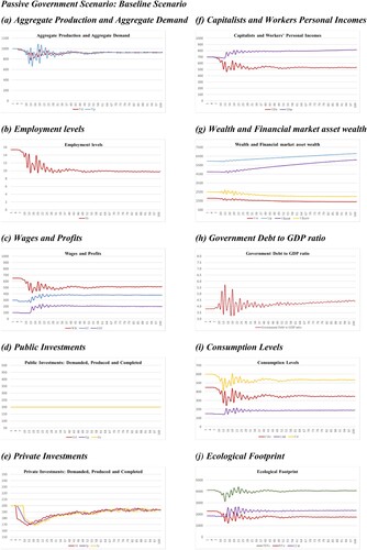
However, while profits are initially reduced by the negative impact of the economic crisis, the reduction in wages and costs allows profits to stop falling and once more increase (Figure 1c). Such a reversed trend in profits stimulates economic activity expectations and, in that way, both demanded and produced private investments, too (Figure 1e). The partial recovery of investments stimulates overall demand and production, together with a slight increase in the wage bill. Such a recovery, however, is not strong enough to restore the pre-crisis wage bill and activity levels. In that way, while the wage bill level remains much lower, total and distributed profits remain higher than the pre-crisis level, thanks to the reduced cost of production (Figure 1c).

Despite the initial volatile periods that occur, mainly due to incorrect expectations,¹⁰ such volatility is increasingly reduced and the resultant dynamics of the previous scenario have a clear impact on overall social distribution between workers and capitalists. In fact, the lower wage bill reduces the workers’ personal income (Figure 1f), which also affects their overall wealth and ability to make financial investments. In the same way, the increased distributed profits obtained by capitalists contribute to their persistently growing higher personal income and, consequently, their higher level of overall and financially investible wealth (Figure 1g). The increase in financially investible wealth stimulates the capitalists’ demand for bills and bonds that are supplied on demand. The increase in government debt — due to the fall in income, which will generate smaller tax payments and therefore a larger government deficit — and a simultaneous reduction in GDP are the main reason for an increased and increasing government debt to GDP ratio (Figure 1h).

Although the crisis did generate a much lower level of economic activity and demand for consumption goods at aggregate level (Figure 1i), it reduced only the consumption levels of workers while increasing that of capitalists, reflecting the distributional effect on disposable income and wealth.

In this way, the EF reduction caused by lower workers consumption is compensated by the increase in the consumption of capitalists. The final effect is a substantially unchanged level of EF (Figure 1j) and more polarized social classes. The economy faced a shift both in the distribution of social classes and the burden of their EF.

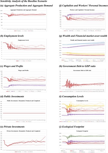
A sensitivity test is conducted (Figure 2) considering weaker (stronger) reactions of the economic agents in response to the exogenous drop in investments compared to the baseline scenario. The values used in the simulation analysis are reported in Table A3.

Figure 2. Sensitivity test of the baseline scenario related to the evolution of macroeconomic, financial, and ecological variables.

Note: The initial values of the variables and parameters used in the simulation analysis are reported in Appendices A–C and Table A3.

4.2. 0BD Government Policy Scenario

In our second scenario, we consider a zero-budget deficit (0BD) policy framework, in which the government tries to achieve constant parity between outlays (pure expenditure plus interest payments on both kinds of debt) and all revenues (tax receipts and central bank profits,$F_{cb}$, which are returned to the government). This policy might be due to the government’s final aim of not letting the public debt/GDP ratio increase above current levels.

However, as Sawyer (2010) clearly pointed out, the budget deficit cannot be controlled exactly by government, potentially persistently frustrating such a policy goal if we consider that, in the end, the budget deficit is actually an endogenous variable:

In effect the budget deficit can be viewed as endogenous and indeed something of a residual … whilst a government can set tax rates and its intentions for public expenditure, the resulting budget deficit arises as a result of decisions made by the private sector and the resulting level of economic activity. (p. 37)

Because it is impossible for the government to calculate the exact amount of public expenditure that would satisfy a constant zero-budget deficit, its best approximation is probably to spend an amount of resources on public investments that would allow a parity of budget if such an amount had been spent in the previous period, according to (93).

In this scenario, the starting dynamics are similar to those in the previous scenario. In fact, as soon as the economy faces the external negative shock in demand for investment, it suffers a decrease in aggregate demand and therefore a decrease in production too (Figure 3a). Such a decrease in production leads to a drop in the employment rate (Figure 3b), which has a further negative impact on aggregate demand. In that way, at first, both the workers’ wage bill and capitalists’ profits drop (Figure 3c), which also decreases their personal incomes (Figure 3f). These decreased personal incomes produce a reduction in taxes collected by the government. In attempting to achieve a zero-budget deficit, the government decreases the amount of public investments available (Figure 3d), which is the biggest difference from the previous scenario. In fact, such a decrease in government expenditure affects the production level (Figure 3d) and, in so doing, decreases the need for employment, lowering the overall employment level even further with respect to the BL (Figure 3b) where the government was not decreasing public expenditure.

Figure 3. Evolution of macroeconomic, financial, and ecological variables. 0BD (bold lines) versus baseline (dotted lines) scenarios.

Note: The initial values of the variables and parameters used in the simulation analysis are reported in Appendices A–C and Table A3.

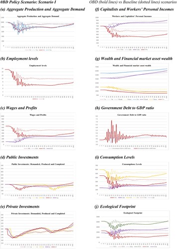
The larger decline in employment makes the wage bill shrink further with respect to the BL (Figure 3c). The lower main cost of production — wages — allows profits finally to increase, stimulating private investment (Figure 3e). Meanwhile, the decreased wage bill and the increased profits affect the personal incomes of the two social classes, contributing to the lowering of the overall and financially investible wealth of the workers, on one side, and increasing the overall and financially investible wealth of the capitalists, on the other (Figure 3f–g).

Even if the recovery of private investment partially attenuates the fall in aggregate demand, its level remains much lower than that in the pre-crisis period, with no significant prospect of increasing again. This situation makes private investments stagnate and slightly decrease (Figure 3e) until the dissociation between demanded, produced and concluded investments becomes relevant again. In fact, although the demand for public investments almost recovered after its first strong decline, concluded public investments also start to fall because of the previous continuously lowered levels of demanded and produced public investments (Figure 3d). Such a fall in concluded public investments decreases public, and thus overall level of, capital stock in the economy.¹¹ The reduced level of capital per worker in the economy leads to a decrease in labour productivity too (via 43), producing two direct effects, namely, reduction of potential output (via 22) and increase in workers needed for production activities (via 34–36). The previous situation puts pressure on capacity utilization and therefore provides a positive stimulus to private investment (Figure 3e). The reactivation of demanded and produced investments mildly supports the employment level, together with wage bill (Figure 3c).

The halting of the declining wage bill together with increased demand for investments finally leads to a light recovery trend for the overall economy. However, there are several differences with respect to the BL scenario. While both the BL and the 0BD aggregate demand and aggregate production levels remain lower than those pre-crisis, in the 0BD scenario those levels stay considerably lower than those of the BL until the end.

The prolonged levels of reduced demand and production cause a consistently lower level of employment that remains significantly lower than the BL scenario too (Figure 3b). The decreased level of employment affects the wage bill, which remains at a lower level with respect to the BL, while it allows firms to reduce their main production costs and thus obtain higher profits. The resultant effect is an even greater polarization of the social classes with respect to both the BL and the pre-crisis situation. In fact, while the higher profit levels produce higher personal incomes for capitalists, thus building up higher levels of overall and financially investible wealth, lower wage bill levels negatively affect workers’ personal income (Figure 3c, f, g).

The 0BD policy did not contribute to reducing the public debt to GDP ratio below the pre-crisis level, while its value remains consistently even higher than the BL (Figure 3h). At the same time, the final aggregate consumption level remains inferior to that achieved in the BL scenario. However, the composition of the demand for consumption goods is quite different. In fact, we can highlight a shift between the consumption of workers and capitalists (Figure 3i) corresponding to their polarized income and disposable wealth. The workers consume less while the capitalists consume more in comparison to the pre-crisis situation and with respect to the BL. This shift in their consumption patterns produces a correspondent shift in their ecological footprint (Figure 3j). As a matter of fact, while the EF of workers is reduced, that of capitalists is higher with respect to the BL. The final overall EF level is higher than the pre-crisis situation and ultimately it is even slightly higher than the BL, with a projection to increase further in future.

4.3. Proactive Government Scenario

In our final scenario we consider a ‘proactive’ government, the final aim of which is to secure a high level of economic activity supporting the aggregated demand level through public social investment. According to this scenario, the government increases its demand for public investment whenever the growth of aggregate demand is lower than a determined minimum threshold, while it decreases demand whenever the growth of aggregate demand exceeds a particular maximum established threshold. Such a government spending policy will be tackled together with a fiscal policy based on taxation. Keynes (1936) perfectly suggested this means of supporting aggregate demand and fighting unemployment by stating that

the remedy would lie in various measures designed to increase the propensity to consume by the redistribution of incomes or otherwise. (p. 324)

The State will have to exercise a guiding influence on the propensity to consume partly through its scheme of taxation, partly by fixing the rate of interest, and partly, perhaps, in other ways. (p. 378)

As previously mentioned (Section 3.6), in such a scenario the government implements a fiscal policy rule so that the tax rates of capitalists and workers decrease whenever their personal incomes fall behind a certain negative growth threshold and increase whenever they exceed a certain positive growth threshold. The aim of such a fiscal policy is to stimulate (calm) their consumption — and therefore overall aggregate demand — whenever economic activity is facing an excessive negative slowdown (or boom). The theoretical background for such a coordinated fiscal policy, that is, to steer the economy whilst simultaneously reducing income inequality, has been suggested and developed by several post-Keynesians, such as Sawyer (2010). The simulation exercises in Figure 4 explore those ideas.

Figure 4. Evolution of macroeconomic, financial, and ecological variables. Proactive (bold lines) versus baseline (dotted lines) scenarios.

Note: The initial values of the variables and parameters used in the simulation analysis are reported in Appendices A–C and Table A3.

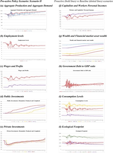
In this scenario, as soon as the exogenous investment shock induces a crisis, the government reacts rapidly by increasing its demand for public investment (Figure 4d), which stimulates overall aggregate demand, thus containing downward instability. Such an idea was previously explored by Fazzari et al. (2013), who argued that, ‘autonomous demand has a profound effect on the model dynamics. It induces a floor that turns around negative dynamics toward growth’ (p. 18). In effect, that demand support directly stimulates the demand for private investments and, consequently, the production of both public and private investments (Figure 4d, e). The overall trend to increase both public and private investment after the crisis leads to a reversed trend in employment required (Figure 4b, period 15), pushing it above the pre-crisis level. Such an effect causes wage levels and therefore the wage bill to increase. At first (see period 20), such a strong increase in wage levels causes a drop in profits, reducing capitalists’ consumption and therefore aggregate demand slightly too. Such a slight drop calls for a further government intervention (see period 22), which again stimulates overall aggregate demand, aggregate production, and level of profits too. The restoration of economic activity continues, also boosting private demanded and produced investments (Figure 4e).

The economic cyclicality characterizing the moment after the exogenous negative shock is reduced by the immediate support of government demand and production but economic trends are quite clear. In fact, the strong intervention of the government via higher demanded and produced public investments generate a positive impact on the overall levels and trajectory of aggregate demand. Increased production stimulates the employment levels that, together with the wage increase, generate an overall positive trend in the wage bill, thus supporting aggregate consumption and overall aggregate demand.

The increase in both capitalist’ profits and workers’ wages induce their personal income to constantly rise. However, following a proactive spending policy, as long as their personal incomes vary, the government manages to change the disposable income patterns of both capitalists and workers by affecting their tax rates. By so doing, the government is able to steer higher levels of the overall and financially investible wealth of both social classes. While the personal incomes of both classes are finally higher than the pre-crisis levels, and projected to increase, their differences in wealth are very much reduced with respect to the pre-crisis, the BL, and the passive government scenarios. The government debt to GDP ratio volatility is much lower with respect to the BL during all the periods under consideration, finally stabilizing its value with a decreasing trend projection.

Overall consumption is finally slightly lower with respect to the pre-crisis levels — such as in the BL scenario — but that alone does not assure a decrease in EF too. In fact, what seems to be relevant for reducing the total EF is also the composition of consumption related to the EF weight of the different social classes. Since the workers have a lower EF weight than the capitalists, even a relevant reduction in workers’ consumption together with an increase in capitalists’ consumption might not assure that an overall decrease in aggregate consumption will lead to an overall reduction in total EF. In fact, in this scenario, the greatest contribution to the reduction of the total EF — with respect to both the pre-crisis and to the BL — comes mainly from the slight reduction in capitalists’ EF.

5. Conclusions

This work developed a post-Keynesian SFC macroeconomic model analysing the dynamics of key socioeconomic variables after a period of a crisis. Our model is built upon Bibi (2020, 2021) within an endogenous money framework and is calibrated using available data for major advanced economies. The model’s framework is characterized by several post-Keynesian features. First, the presence of two social classes, capitalists and workers, with different consumption behaviours and different endowments. Second, the differing consumption behaviours of workers and capitalists have an impact on resources needed and affect ecological balance. Third, non-financial firms and also government can undertake investment decisions and both accumulate capital. Through simulations, different policy scenarios are investigated in which the government might use different fiscal policy rules and tools to achieve recovery in a sustainable way. Socioeconomic sustainability is here interpreted in terms of reduced unemployment, a less polarized society and ecological sustainability proxied by the ecological footprint.

In particular, three different policy scenarios were investigated as a reaction to an exogenous fall in private investment. First, we considered a situation in which the government does not change its expenditure despite the negative exogenous shock (our baseline scenario). We then analysed a policy scenario whereby the government pursued a zero-budget deficit (OBD) policy rule with the final aim of not letting the public debt to GDP ratio increase. Finally, the third situation was represented by a proactive policy scenario whereby the government implemented its main fiscal policies — spending and taxation — to support economic activity following a functional finance approach.

The analysis was carried out using an SFC model that takes into account all monetary connections within the economy among the different sectors and between the two social classes, too. This work contains some interesting novelties with respect to the existing literature. While few SFC models explicitly consider an economy formed by two social classes, no one — to our knowledge — considers the impacts of the Kaleckian temporal lags among demanded, produced and concluded private investments in such a framework. Second, while SFC models generally consider the government sector, rarely do any consider its role in demanding and producing social public investments that, together with private investments, form the overall capital endowment of an economy. Such analysis is relevant to stress the divergence in outcomes sought for engagement in investment projects: for the private sector, it is driven mainly by the desire to increase production capacity and ultimately profit; for the public sector, it is motivated by a functional finance approach, increasing the capital of the overall economy and using public expenditure as a tool to support demand in periods of recession too. Finally, combining those Kaleckian ideas with those of Keynesians regarding the ways in which a government can restore the economy through government spending and taxes, we highlighted how investment decisions such as consumption patterns might be steered to ensure economic and social recovery in a sustainable ecological way. Our model draws some relevant conclusions in terms of the key indicators of an economy after an exogenous drop in demand. Fiscal policies adopted by the government were studied, together with the recovery path followed by the economy, the employment level, and wage and wealth distribution between social classes, and some simple ecological inferences made. In the passive government policy scenario (BL), the lack of reactiveness in terms of fiscal expenditure meant it was unable to restore the economy to its pre-crisis situation regarding aggregate production and employment, with a further polarization of the social classes in terms of income and wealth. Overall economic consumption falls but, as a result of the redistribution in consumption and because of the different EF weights of the social classes, an overall reduction in ecological impact is not necessarily guaranteed. In the 0BD scenario, the austerity measures cause a worse outcome in terms of restoration of economic activity and employment with respect to the BL, with even more polarized distribution between the social classes in terms of both income and wealth. In fact, the policy rule — that the government pursues here — leads the government to contract its expenditure, inducing aggregate demand, production, and employment to contract even further. For the whole period considered, the indicators of the real side of the economy remain much lower than in both the pre-crisis situation and the BL scenario. If the total EF remains inferior to that in the BL scenario during most of the simulated period, its value finally reaches the BL level with a clear tendency to surpass it. As in the BL scenario, in the 0BD scenario the government is not able to avoid increasing the debt/GDP ratio even if this was the ultimate goal of its policy. Finally, in the proactive government policy scenario, the countercyclical reaction of government expenditure enables economic activity to be supported and to reverse the fall of the main real macroeconomic variables. A further polarization of the social classes is avoided and, in fact, even reduced. However, such a result is obtained without imposing a cut on the income or wealth of either social classes. The personal incomes and wealth of both workers and capitalists increase while reduced consumption allows the total EF to be reduced. Increased production contributes to stabilizing the government debt/GDP ratio.

Our model can be expanded in several ways. First, further features of the ecological balance might be incorporated to also include the effects of damage functions. Second, future investigations could research the space for monetary or combined policies able to achieve a similar social, economic, and ecological sustainable scenario. Third, country-specific analysis might further consider this work by applying specificities of developed or developing countries.

Acknowledgements

I would like to use this opportunity to acknowledge and thank the reviewers who reviewed this article and aided in its publication. I am grateful to Malcolm Sawyer and Stefano Zambelli who accompanied me during the journey of my PhD, as well as to the Editor and the two anonymous referees for their suggestions and comments to the present work that allowed me to deeply shape and improve it. I am also grateful to Diego Guevara, Marco Veronese Passarella and Gennaro Zezza for the support they provide at the beginning of this work. Any remaining errors or omissions are strictly my own.

Disclosure Statement

No potential conflict of interest was reported by the author.

Notes

1 To avoid any confusion between commercial banks and the central bank, we call CBs the former and CCB (country central bank) the latter.

2 For simplicity, we will often call the investment goods that firms sell to the government ‘public investments’.

3 The ecological footprint is a ‘measure of how much area of biologically productive land and water an individual, population or activity requires to produce all the resources it consumes and to absorb the waste it generates, using prevailing technology and resource management practices’ (Global Footprint Network 2015). This simple approach to ecological sustainability is intended to give just an idea of the effects that different consumption structures have in relation to the depletion of resources. A much deeper and more comprehensive consideration of ecosystem-related variables is contained in Dafermos et al. (2017), where, for example, there is a differentiation between conventional and green investments and where the degradation of ecosystem services has feedback effects on the economy.

4 Mackenzie et al. (2008) also show how, while in general the size of an individual ecological footprint increases as household income increases, the real jump is at the top 10 per cent level. In housing and transportation, in particular, the ecological footprint of the richest 10 per cent of Canadian households is several times the size of the footprint of lower — and lower-middle-income Canadians and significantly greater than that of the next highest-income 10 per cent of households. According to collected data, the richest decile consumes more than nine times that of the poorest decile.

5 Equations 1–4, 9–10 and 23–25 are taken from the analysis presented in the Macroeconomics and Monetary System module at Trento University (Zambelli 2014).

6 This assumption is in line with the idea that firms are not willing to change their prices unless their unit costs change significantly.

7 The main reason for this assumption is to stress the goal divergence of the investment projects demanded by the private sector (driven mainly by the desire to increase production capacity and ultimately profit) and those demanded by the public sector (driven by a functional finance approach, increasing the capital of the overall economy and also using public expenditure as a tool to support demand in periods of recession). This is just a simplification hypothesis, which might be altered in future research projects in line with this work. It is assumed that the government spends only by purchasing investment goods and not on current expenditure. This too is a simplification that may be modified in future.

8 These policy scenario simulations are based on Bibi (2021) and this work intends to expand that by analysing the same policies and their implications through a comprehensive analysis within the features of an SFC model.

9 The model is calibrated using available data for major advanced economies (for example, the different marginal propensities to consume of workers and capitalists, different coefficients for their ecological footprints, coefficients of wage reactions to changes in unemployment levels) and reasonable values (such as proportions of C, I, G, and the wage bill upon GD together with parameters adopted by previous literature). The initial values of the variables and parameters used in the simulation analysis are reported in the appendices and Table A3.

10 The main source of volatility derives from the larger values allowed to be taken from ${\eta }^{\mathrm{\prime }}$. With smaller values of ${\eta }^{\mathrm{\prime }}$, volatility would be reduced even if the main results are maintained. Bibi (2020) provides a deeper explanation of the volatility of the main variables in the model, which is related to the expectations of firms (${\eta }^{\mathrm{\prime }}$), the interaction between the sensitivity of wages to the variation of EPL (${\gamma }_z$), the sensitivity of wages to the variation of the unemployment level (${\gamma }_u$), and the sensitivity of workers’ productivity to variations in wages (${\gamma }_w$). Despite the volatility in the production of consumption goods initially affecting all other variables, such volatility is reduced with time and the main variable trends are clearly visible.

11 In fact, the simulated data show that, while total capital levels were slowly increasing again after the crisis up to period 56 (thanks to the recovery of private capital), period 57 demarks the reduction of public capital that — due to its magnitude — negatively affects the level of total capital (values not represented in the charts).

Appendix A.

Balance Sheet Matrix, Transaction-Flow Matrix, Equations list and values of key parameters.

Table A1. Balance sheet matrix.

	Households		Production firms	Government	Central bank	Banks	∑
	Workers	Capitalists
Inventories			$+IN$				$+IN$
Fixed capital			$+K^I$	$+K^G$			$+K^T$
HPM (cash)	$+H_w$	$+H_{\pi }$			$-H$	$+H_b$	0
Money (deposit)	$+M_w$	$+M_{\pi }$				$-M$	0
Bills		$+B_{\pi }$		$-B$	$+B_{cb}$	$+B_b$	0
Bonds		$+B{L}_{\pi }\cdot p_{bL}$		$-B{L}_{\pi }\cdot p_{bL}$			0
Loans	$-L_w$	$-L_{\pi }$	$-L_f$			$+L$	0
Bank capital		$+O{F}_b$				$-O{F}_b$	0
Balance (net worth)	$-V_w$	$-V_{\pi }$	$-V_f$	$-V_g$	0	0	$-\left(IN+K\right)$
∑	0	0	0	0	0	0	0

Table A2. Transaction-flow matrix.

	Households		Firms		Government		Central bank		Banks		∑
	Workers (1)	Capitalists (2)	Current (3)	Capital (4)		Current (5)	Capital (6)	Current (7)	Capital (8)	Current (9)
Consumption	$-C_w^D$	$-C_{\pi }^D$	$+C^D$								0
Government expenditure					$-G^D$						0
Government Expenditure			$+G^D$								0
Fixed investment			$+I^D$	$-I^D$							0
Inventory accumulation											0
Taxes	$-T_w$	$-T_{\pi }$			+T						0
Wages	+WB		−WB								0
Inventory financing cost			$-r_{l-1}\cdot I{N}_{-1}$						$+r_{l-1}\cdot I{N}_{-1}$		0
Entrepreneurial profits		$+F{D}_f$	$-F_f$	$+F{U}_f$					$+r_{l-1}\cdot \left(L_{f-1}-I{N}_{-1}\right)$		0
Bank profits		$+F_b$							$-F_b$		0
Central bank profits					$+F_{cb}$		$-F_{cb}$				0
Loan interest	$-r_{l-1}\cdot L_{w-1}$	$-r_{l-1}\cdot L_{\pi -1}$							$+r_{l-1}\cdot L_{h-1}$		0
Deposit interest	$+r_{m-1}\cdot M_{w-1}$	$+r_{m-1}\cdot M_{\pi -1}$							$-r_{m-1}\cdot M_{-1}$		0
Bill interest		$+r_{b-1}\cdot B_{\pi -1}$			$-r_{b-1}\cdot B_{-1}$		$+r_{b-1}\cdot B_{cb-1}$		$+r_{b-1}\cdot B_{b-1}$		0
Bond interest		$+B{L}_{-1}$			$-B{L}_{-1}$						0
Flows of funds (changes in stocks)
Change in loans	$+\mathrm{\Delta }{L}_w$	$+\mathrm{\Delta }{L}_{\pi }$		$+\mathrm{\Delta }{L}_f$						$-\mathrm{\Delta }L$	0
Change in HPM (cash)	$-\mathrm{\Delta }{H}_w$	$-\mathrm{\Delta }{H}_{\pi }$						$+\mathrm{\Delta }H$		$-\mathrm{\Delta }{H}_b$	0
Change in money (deposits)	$-\mathrm{\Delta }{M}_w$	$-\mathrm{\Delta }{M}_{\pi }$								$+\mathrm{\Delta }M$	0
Change in bills		$-\mathrm{\Delta }{B}_{\pi }$			$+\mathrm{\Delta }B$			$-\mathrm{\Delta }{B}_{cb}$		$-\mathrm{\Delta }{M}_b$	0
Change in bonds		$-\mathrm{\Delta }BL\cdot p_{bL}$			$+\mathrm{\Delta }BL\cdot p_{bL}$						0
∑	0	0	0	0	0	0	0	0	0	0	0

Table A3. Values of the key parameters in the baseline scenario, in the sensitivity test, in scenario I and in scenario II.

Values of key parameters in the sensitivity and policy analysis
Parameter		Baseline scenario	Sensitivity test I	Sensitivity test II	OBD Ggvernment (scenario I)	Proactive government (scenario II)	Notes
Adjustment workers mpcW parameter	${\gamma }_{c\pi 1}$	0.800	0.600	1.000	0.800	0.80	In Sensitivity test I (Sensitivity test II) weaker (stronger) reaction parameters respect to the Baseline scenario are considered. In the 0 Budget Deficit policy (0BD, scenario I), the Government try to achieve a 0 Budget Deficit demanding an amount of Government expenditure such that the Budget Deficit of the previous period could have been nil. In the Proactive policy (scenario II) the government implements a fiscal policy such that capitalists and workers’ tax rates decrease (increase) when their personal incomes fall behind (exceed) a certain degrowth (growth) threshold with the aim of stimulate (calm) their consumption and in this way the economic activity. With the same intention, Government expenditure increase (decrease) when the aggregate demand fall behind (exceed) a certain degrowth (growth) threshold.
Adjustment capitalists mpcW parameter	${\gamma }_{cw2}$	1.500	1.200	1.800	1.500	1.50
Coefficient of w reaction to change in z	${\gamma }_z$	0.200	0.100	0.300	0.200	0.20
Coefficient of (+)w reaction to change in (−)u	${\gamma }_{u-}$	0.500	0.200	0.800	0.500	0.50
Coefficient of (−)w reaction to change in (+)u	${\gamma }_{u+}$	0.250	0.100	0.400	0.250	0.25
Coefficient of A reaction to change in w	${\gamma }_w$	0.500	0.080	0.700	0.500	0.50
Coefficient of A reaction to change in (K/N)	${\gamma }_{L+}$	0.300	0.275	0.325	0.300	0.30
Labour force reaction to change in (+)Yd	${\gamma }_{L-}$	0.250	0.200	0.300	0.250	0.25
Labour force reaction to change in (−)Yd	$a_1$	0.250	0.200	0.300	0.250	0.25
Expected investment parameter	$a_2$	0.100	0.080	0.120	0.100	0.10
cu parameter related to investment	$a_3$	0.012	0.010	0.014	0.012	0.012
Weight to previous level of profits	$a_4$	0.100	0.040	0.160	0.100	0.10
Weight to previous change in profits	${\psi }_L$	1.000	0.200	1.800	1.000	1.00
Capacity output growth wrt L		2.000	1.000	3.000	2.000	2.00
Capacity output growth wrt A	${\psi }_A$ ${\zeta }_m$	2.000	1.000	3.000	2.000	2.00
Change in deposit rate reaction parameter		0.00020	0.00020	0.00025	0.00020	0.0002
Adjustment workers tax parameter	${\gamma }_{\tau w}$ ${\gamma }_{\tau \pi }$	0	0	0	0	0.5
Adjustment capitalists tax parameter		0	0	0	0	0.3
Threshold of (+)w to let w tax increase	${\phi }_{\tau wh\left(high\right)}$ ${\phi }_{\tau \pi h\left(high\right)}$	0.0%	0.0%	0.0%	0.0%	0.5%
Threshold of (+)π to let π tax increase	${\phi }_{\tau whl\left(low\right)}$	0.0%	0.0%	0.0%	0.0%	0.5%
Threshold of (−)w to let w tax decrease	${\phi }_{\tau \pi l\left(low\right)}$	0.0%	0.0%	0.0%	0.0%	−6.0%
Threshold of (−)π to let π tax decrease	${\gamma }_{g(-)}$	0.0%	0.0%	0.0%	0.0%	−7.0%
Variation of (−)government intervention	${\gamma }_{g(+)}$	0	0	0	0	0
Variation of (+)government intervention	${\phi }_{Gl\left(low\right)}$	0	0	0	0	0.75
Threshold of (−)Yd to let government +G	${\phi }_{Gh\left(high\right)}$	0.0%	0.0%	0.0%	0.0%	0.0%
Threshold of (+)Yd to let government −G		0.0%	0.0%	0.0%	0.0%	5.0%

Equations used in the model. (1) $Y^D=C^D+I^D+G^D$(1) (2) $Y^P=C^P+I^P+G^P$(2) (3) $C^P=E_{-1}\left(C^D\right)+s^{\ast }$(3) (4) $E_{-1}\left(C^D\right)=C_{-1}^D+{\eta }^{\mathrm{\prime }}\left(C_{-1}^D-C_{-2}^D\right)$(4) (5) ${\eta }^{\mathrm{\prime }}={\displaystyle \frac{C_{-1}^D-C_{-2}^D}{C_{-2}^D-C_{-3}^D}}$(5) (6) ${\eta }^{\mathrm{\prime }}=0if{C}_{-2}^D=C_{-3}^D$(6) (7) ${\eta }^{\mathrm{\prime }}={\eta }_L^{\mathrm{\prime }}if{\displaystyle \frac{C_{-1}^D-C_{-2}^D}{C_{-2}^D-C_{-3}^D}<{\eta }_L^{\mathrm{\prime }}}$(7) (8) ${\eta }^{\mathrm{\prime }}={\eta }_U^{\mathrm{\prime }}if{\displaystyle \frac{C_{-1}^D-C_{-2}^D}{C_{-2}^D-C_{-3}^D}\ge {\eta }_U^{\mathrm{\prime }}}$(8) (9) $s^{\ast }=\alpha E_{-1}\left(C^D\right)-Q_{-1}$(9) (10) $Q=s+Q_{-1}=C^P-C^D+Q_{-1}$(10) (11) $IN=Q\cdot UC$(11) (12) $I^D=I_{-1}^D+a_1\cdot {\pi }_{\left(t+1\right)}^e\cdot I_{-1}^D+a_2\cdot c{u}_{-1}\cdot I_{-1}^D$(12)

(13) ${\pi }_{\left(t+1\right)}^e={\displaystyle \frac{{\pi }_{\left(t+1\right)}^e}{Y^D}}$(13) (14) ${\pi }_{\left(t+1\right)}^e=a_3\cdot F_f-1+a_4\cdot \left(F_f-1-F_f-2\right)$(14) (15) $a_1=+\left|a_1\right|if\left(F_f-1-F_f-2\right)>0$(15) (16) $a_1=-\left|a_1\right|if\left(F_f-1-F_f-2\right)<0$(16) (17) $a_1=0if\left(F_f-1-F_f-2\right)=0$(17) (18) $a_2=+\left|a_2\right|if\left(Y_{-1}^D-Y_{-2}^D\right)>0$(18) (19) $a_2=-\left|a_2\right|if\left(Y_{-1}^D-Y_{-2}^D\right)<0$(19) (20) $a_2=0if\left(Y_{-1}^D-Y_{-2}^D\right)=0$(20) (21) $cu={\displaystyle \frac{Y^D}{Y^{\ast }}}$(21) (22) $Y^{\ast }=Y_{-1}^{\ast }+{\psi }_L\cdot \left({\displaystyle \frac{L^T-L_{-1}^T}{L_{-1}^T}}\right)\cdot Y_{-1}^{\ast }+{\psi }_A\cdot \left({\displaystyle \frac{A-A_{-1}}{A_{-1}}}\right)\cdot Y_{-1}^{\ast }$(22) (23) $I^P={\displaystyle \frac{1}{{\theta }_I}\sum _{j=1}^{\theta }{I}_{\left(-1-\theta +j\right)}^D}$(23) (24) $I^C=I_{-{\theta }_I}^D$(24) (25) $K^I=K_{-1}^I-{\delta }_{KI}\cdot K_{-1}^I+I^C$(25) (26) $C^P=A{N}^C$(26) (27) $I^P=A{N}^I$(27) (28) $w=w_{-1}+{\gamma }_z\cdot {\displaystyle \frac{z-z_{-1}}{z_{t-1}}\cdot w_{-1}-{\gamma }_u\cdot \left(u_{-1}-u_{-2}\right)\cdot w_{-1}}$(28) (29) ${\gamma }_u={\gamma }_{u-}if\left(u_{-1}-u_{-2}\right)>0$(29) (30) ${\gamma }_u={\gamma }_{u+}if\left(u_{-1}-u_{-2}\right)<0$(30) (31) ${\gamma }_u=0if{u}_{-1}=u_{-2}$(31) (32) $WB=w\cdot N^T$(32) (33) $p_y=\left(1+\rho \right)\left({\displaystyle \frac{w}{A_{}}}\right)$(33) (34) $\rho =\left({\displaystyle \frac{Y^D}{WB}}\right)-1$(34) (35) $N^C={\displaystyle \frac{C^P}{A}}$(35) (36) $N^I={\displaystyle \frac{I^P}{A}}$(36)

(37) $N^G={\displaystyle \frac{G^P}{A}}$(37) (38) $N^T=N^C+N^I+N^G$(38) (39) $u={\displaystyle \frac{U}{LF}={\displaystyle \frac{LF-N^T}{LF}=1-{\displaystyle \frac{N^T}{LF}}}}$(39)

(40) $LF=L{F}_{-1}+{\gamma }_L\cdot {\displaystyle \frac{Y_{-1}^D-Y_{-2}^D}{Y_{-2}^D}\cdot L{F}_{-1}}$(40) (41) ${\gamma }_L={\gamma }_{L-}if{\displaystyle \frac{Y_{-1}^D-Y_{-2}^D}{Y_{-2}^D}<0}$(41) (42) ${\gamma }_L={\gamma }_{L+}if{\displaystyle \frac{Y_{-1}^D-Y_{-2}^D}{Y_{-2}^D}>0}$(42) (43) ${\gamma }_L=0if{\displaystyle \frac{Y_{-1}^D-Y_{-2}^D}{Y_{-2}^D}=0}$(43) (44) $A=A_{-1}+{\gamma }_{\omega }\cdot \left({\displaystyle \frac{w-w_{-1}}{w_{-1}}}\right)\cdot A_{-1}+{\gamma }_k\cdot \left({\displaystyle \frac{{\displaystyle \frac{K_{-1}^T}{N_{-1}^T}-{\displaystyle \frac{K_{-2}^T}{N_{-2}^T}}}}{{\displaystyle \frac{K_{-1}^T}{N_{-1}^T}}}}\right)\cdot A_{-1}$(44) (45) $UC={\displaystyle \frac{WB}{A}}$(45) (46) $F_f=Y^D-WB+\mathrm{\Delta }IN-r_l\cdot I{N}_{-1}$(46)

(47) $F{D}_f={\psi }_D\cdot F_{f-1}if{L}_{fd-1}>{\psi }_{IN}\cdot I{N}_{-1}$(47) (48) $F{D}_f=F_f-F{U}_f-r_l\cdot (L_{fd-1}-I{N}_{-1})if{L}_{fd-1}\le {\psi }_{IN}\cdot I{N}_{-1}$(48) (49) $F{U}_f=F_f-F{D}_f-r_l\cdot (L_{fd-1}-I{N}_{-1})if{L}_{fd-1}>{\psi }_{IN}\cdot I{N}_{-1}$(49) (50) $F{U}_f=I^{D}if{L}_{fd-1}\le {\psi }_{IN}\cdot I{N}_{-1}$(50) (51) $L_{fd}=L_{fd-1}+I^D+\mathrm{\Delta }IN-F{U}_f$(51) (52) $Y{P}_w=WB+r_{m-1}\cdot M_{w-1}$(52) (53) $Y{P}_{\pi }=F{D}_f+F{D}_b+r_{m-1}\cdot M_{\pi -1}+r_{b-1}\cdot B_{\pi d-1}+B{L}_{\pi d-1}$(53) (54) $Y{D}_w=Y{P}_w-T_w-r_{l-1}\cdot L_{w-1}$(54) (55) $Y{D}_{\pi }=Y{P}_{\pi }-T_{\pi }-r_{l-1}\cdot L_{\pi -1}$(55) (56) $T_w={\tau }_w\cdot Y{P}_{w-1}$(56) (57) $T_{\pi }={\tau }_{\pi }\cdot Y{P}_{\pi -1}$(57)

(58) $V_w=V_{w-1}+Y{D}_w-C_w^D$(58) (59) $V_{\pi }=V_{\pi -1}+Y{D}_{\pi }-C_{\pi }^D$(59) (60) $C_w^D=c_{w1}\cdot (Y{D}_{w-1}+N{L}_{sw-1})+c_{w2}\cdot V_{w-1}$(60) (61) $C_{\pi }^D=c_{\pi 1}\cdot (Y{D}_{\pi -1}+N{L}_{\pi -1})+c_{\pi 2}\cdot V_{\pi -1}$(61) (62) $c_{w1}=c_{w1-1}-{\gamma }_{cw1}{\displaystyle \frac{{\tau }_{w-1}-{\tau }_{w-2}}{{\tau }_{w-2}}\cdot c_{w1-1}}$(62) (63) $c_{\pi 1}=c_{\pi 1-1}-{\gamma }_{c\pi 1}{\displaystyle \frac{{\tau }_{\pi -1}-{\tau }_{\pi -2}}{{\tau }_{\pi -2}}\cdot c_{\pi 1-1}}$(63) (64) $C^D=C_w^D+C_{\pi }^D$(64) (65) $E{F}_w={\phi }_w\cdot C_w^D$(65) (66) $E{F}_{\pi }={\phi }_{\pi }\cdot C_{\pi }^D$(66) (67) $TEF=E{F}_w+E{F}_{\pi }$(67) (68) $G{L}_T=G{L}_{\pi }+G{L}_w$(68) (69) $G{L}_{\pi }=\text{β}\cdot Y{P}_{\pi }$(69) (70) $G{L}_w=\text{β}\cdot Y{P}_w$(70) (71) $\text{β}={\text{β}}_0-{\text{β}}_r\cdot r_l$(71) (72) $N{L}_{\pi }=G{L}_{\pi }-RE{P}_{\pi }$(72) (73) $N{L}_w=G{L}_w-RE{P}_w$(73) (74) $RE{P}_{\pi }={\xi }_{\pi }\cdot L_{h\pi d-1}$(74) (75) $RE{P}_w={\xi }_w\cdot L_{hwd-1}$(75) (76) $L_{hd}=L_{h\pi d}+L_{hwd}$(76) (77) $L_{h\pi d}=L_{h\pi d-1}+N{L}_{\pi }$(77) (78) $L_{hwd}=L_{hwd-1}+N{L}_w$(78) (79) $\left[\begin{array}{c}{\displaystyle \frac{M_{\pi d}}{V_{fma\pi -1}}}\\ {\displaystyle \frac{B_{\pi d}}{V_{fma\pi -1}}}\\ {\displaystyle \frac{\left(p_{bL}\cdot B{L}_{\pi d}\right)}{V_{fma\pi -1}}}\end{array}\right]=\left[\begin{array}{c}\lambda {\pi }_{10}\\ \lambda {\pi }_{20}\\ \lambda {\pi }_{30}\end{array}\right]+\left[\begin{array}{ccc}{\lambda }_{\pi 11}& {\lambda }_{\pi 12}& {\lambda }_{\pi 13}\\ {\lambda }_{\pi 21}& {\lambda }_{\pi 22}& {\lambda }_{\pi 23}\\ {\lambda }_{\pi 31}& {\lambda }_{\pi 32}& {\lambda }_{\pi 33}\end{array}\right]\left[\begin{array}{c}{r}_m\\ r_b\\ r_{bL}\end{array}\right]+\left[\begin{array}{c}{\lambda }_{\pi 14}\\ {\lambda }_{\pi 24}\\ {\lambda }_{\pi 34}\end{array}\right]Y{P}_{\pi }$(79) $\lambda {\pi }_{10}+\lambda {\pi }_{20}+\lambda {\pi }_{30}=1\left(\mathrm{A}\mathrm{C}1\right)$ $\lambda {\pi }_{11}+\lambda {\pi }_{21}+\lambda {\pi }_{31}=0\text{ł}\left(\mathrm{A}\mathrm{C}2\right)$ $\lambda {\pi }_{12}+\lambda {\pi }_{22}+\lambda {\pi }_{32}=0\left(\mathrm{A}\mathrm{C}3\right)$ $\lambda {\pi }_{13}+\lambda {\pi }_{23}+\lambda {\pi }_{33}=0\left(\mathrm{A}\mathrm{C}4\right)$

$\lambda {\pi }_{14}+\lambda {\pi }_{24}+\lambda {\pi }_{34}=0\left(\mathrm{A}\mathrm{C}5\right)$ $\lambda {\pi }_{11}=-(\lambda {\pi }_{12}+\lambda {\pi }_{13})=0\left(\mathrm{A}\mathrm{C}6\right)$ $\lambda {\pi }_{22}=-(\lambda {\pi }_{21}+\lambda {\pi }_{23})=0\left(\mathrm{A}\mathrm{C}7\right)$ $\lambda {\pi }_{33}=-(\lambda {\pi }_{31}+\lambda {\pi }_{32})=0\left(\mathrm{A}\mathrm{C}8\right)$ (79) $M_{wd}=V_{fmaw-1}$(79) (80) $M_{\pi h}=V_{fma\pi }-B_{\pi d}-p_{bL}\cdot B{L}_{\pi d}$(80) (81) $M_{wh}=V_{fmaw}$(81) (82A) $V_{fma\pi }=M_{\pi d}+B_{\pi d}+p_{bL}\cdot B{L}_{\pi d}$(82A) (82) $V_{fma\pi }=V_{\pi }+L_{\pi d}-H_{\pi d}-OF$(82) (83A) $V_{fmaw}=M_{wd}$(83A) (83) $V_{fmaw}=V_w+L_{wd}-H_{wd}$(83) (84) $H_{\pi d}={\lambda }_{c\pi }\cdot C_{\pi }^D$(84) (85) $H_{wd}={\lambda }_{cw}\cdot C_w^D$(85) (86) $T_T=T_w+T_{\pi }$(86) (55) $T_w={\tau }_w\cdot Y{P}_{w-1}$(55) (56) $T_{\pi }={\tau }_{\pi }\cdot Y{P}_{\pi -1}$(56) (87) ${\tau }_w={\tau }_{w-1}+{\gamma }_{\tau w}\cdot \left(\left|{\displaystyle \frac{Y{P}_{w-1}-Y{P}_{w-2}}{Y{P}_{w-1}}}\right|\right)\cdot {\tau }_{w-1}$(87) (88) ${\tau }_{\pi }={\tau }_{\pi -1}+{\gamma }_{\tau \pi }\cdot \left(\left|{\displaystyle \frac{Y{P}_{\pi -1}-Y{P}_{\pi -2}}{Y{P}_{\pi -1}}}\right|\right)\cdot {\tau }_{\pi -1}$(88) (89) ${\gamma }_{\tau w}=+\left|{\gamma }_{\tau w}\right|if{\displaystyle \frac{Y{P}_{w-1}-Y{P}_{w-2}}{Y{P}_{w-1}}>{\phi }_{\tau wh}}$(89) (90) ${\gamma }_{\tau \pi }=+\left|{\gamma }_{\tau \pi }\right|if{\displaystyle \frac{Y{P}_{\pi -1}-Y{P}_{\pi -2}}{Y{P}_{\pi -1}}>{\phi }_{\tau \pi h}}$(90) (91) ${\gamma }_{\tau w}=-\left|{\gamma }_{\tau w}\right|if{\displaystyle \frac{Y{P}_{w-1}-Y{P}_{w-2}}{Y{P}_{w-1}}\le {\phi }_{\tau wl}}$(91) (92) ${\gamma }_{\tau \pi }=-\left|{\gamma }_{\tau \pi }\right|if{\displaystyle \frac{Y{P}_{\pi -1}-Y{P}_{\pi -2}}{Y{P}_{\pi -1}}\le {\phi }_{\tau \pi l}}$(92) (93) $G^D=G_{-1}^D$(93) (93A) $G^D=G_{-1}^D-PSB{R}_{-1},G^D\ge 0$(93A) (93B) $G^D=G_{-1}^D+{\gamma }_g\cdot \left(\left|{\displaystyle \frac{Y_{-1}^D-Y_{-2}^D}{Y_{-2}^D}}\right|\right)\cdot G_{-1}^D,G^D\ge 0$(93B)

(94) $G^P={\displaystyle \frac{1}{{\theta }_G}\sum _{j=1}^{\theta }{G}_{\left(-1-\theta +j\right)}^D}$(94) (95) $G^C=G_{\left(-{\theta }_G\right)}^D$(95) (96) $K^G=K_{-1}^G-{\delta }_{KG}\cdot K_{-1}^G+G^C$(96) (97) $K^T=K^I+K^G$(97) (98) $G^P=A{N}^G$(98) (99) ${\gamma }_g=+\left|{\gamma }_g\right|if{\displaystyle \frac{Y_{t-1}^D-Y_{t-2}^D}{Y_{t-2}^D}\le {\phi }_{Gl}}$(99) (100) ${\gamma }_g=-\left|{\gamma }_g\right|if{\displaystyle \frac{Y_{t-1}^D-Y_{t-2}^D}{Y_{t-2}^D}>{\phi }_{Gh}}$(100) (101) ${\gamma }_g=0elseif$(101) (102) $PSBR=G^D+r_{b-1}\cdot \left(B_{\pi s-1}+B_{bs-1}\right)+B{L}_{\pi s-1}-T_T$(102) (103) $B_s=B_{s-1}+PSBR-\mathrm{\Delta }B{L}_{\pi s}.p_{bL}$(103) (104) $GD=B_{\pi s}+B{L}_{\pi s}+H_s$(104) (105) $F_{cb}=r_{b-1}\cdot B_{cbd-1}$(105) (106) $B{L}_{\pi s}=B{L}_{\pi d}$(106) (107) $B_{\pi s}=B_{\pi d}$(107) (108) $H_{hs}=H_{\pi d}+H_{wd}$(108) (109) $H_{bs}=H_{bd}$(109) (110) $H_s=H_{bs}+H_{hs}$(110) (111) $B_{cbd}=H_s$(111) (112) $B_{cbs}=B_{cbd}$(112) (113) $r_b={\overline{r}}_b$(113) (114) $r_{bL}=r_b+ad{d}_{BL}$(114) (115) $p_{bL}={\displaystyle \frac{1}{r_{bL}}}$(115) (116) $M_s=M_h$(116) (117) $L_{fs}=L_{fd}$(117) (118) $L_{hs}=L_{hd}$(118) (119) $H_{bd}={\rho }_b\cdot M_s$(119) (120) $B_{bs}=B_s-B_{hs}-B_{cbs}$(120)

(121) $B_{bd}=M_s-L_{fs}-L_{hs}-H_{bd}+O{F}_b$(121) (122) $BLR={\displaystyle \frac{B_{bd}}{M_s}}$(122) (123) $r_m=r_{m-1}+\mathrm{\Delta }{r}_m$(123) (124) $\mathrm{\Delta }{r}_m={\zeta }_m\cdot \left(z_1-z_2\right)$(124) (125) $z_1=1iffBLR<bot$(125) (126) $z_2=1iffBLR>top$(126) (127) $r_l=r_m+ad{d}_1$(127) (128) $F_b=r_{l-1}\cdot \left(L_{fs-1}+L_{hs-1}\right)+r_{b-1}\cdot B_{bd-1}-r_{m-1}\cdot M_{s-1}$(128) (129) $OF=O{F}_{-1}$(129) (130) $B_{bd}=B_{bs}$(130)

Appendix B.

Initial values of endogenous variables

Table

Symbol	Description	Value	Remarks/sources
$A$	Labour productivity	65	Calibrated such that the model generates the baseline scenario described in Section Four
$B_{bd}$	Bills demanded by banks (balance-sheet constraint of banks)	2,500	Calculated from Equation (121) using the initial values of $M_s$, $L_{fs}$, $L_{hs}$, $H_{bd}$ and $O{F}_b$
$B_{bs}$	Household bills supplied on demand	2,500	Calculated from Equation (120) using the initial values of $B_s$, $B_{hs}$ and $B_{cbs}$
$B_{cbd}$	Demand of central bank bills	2,500	Calculated from Equation (111) using the initial values of $H_s$
$B_{cbs}$	Supply of central bank bills	2,500	Calculated from Equation (112) using the initial values of $B_{cbd}$
$B_s$	Government bills	6,250	Calibrated such that the model generates the baseline scenario described in Section Four
$B_{\pi d}$	Bills demanded by capitalists	1,250	Selected from a reasonable range of values in relation to $V_{fma\pi }$ and respecting the condition of Equation (78)
$B_{\pi s}$	Bills supplied to capitalists on demand	1,250	Calculated from Equation (107) using the initial values of $B_{\pi d}$
$BLR$	Bank liquidity ratio	0.50	Calculated from Equation (122) using the initial values of $B_{bd}$ and $M_s$
$B{L}_{\pi d}$	Long-term bonds demanded by capitalists	1,000	Selected from a reasonable range of values in relation to $V_{fma\pi }$ and respecting the condition of Equation (78)
$B{L}_{\pi s}$	Bond supplied to capitalists	50	Calculated from Equation (106) using the initial values of $B{L}_{\pi d}$
$C^D$	Total demand for consumption goods	600	Calculated from Equation (63) using the initial values of $C_w^D$ and $C_{\pi }^D$
$C_w^D$	Demand for consumption goods by workers	450	Calculated from Equation (59) using the initial values of $c_{w1}$, $Y{D}_w$, $N{L}_w$, $c_{w2}$ and $V_w$
$C_{\pi }^D$	demand for consumption goods by capitalists	150	Calculated from Equation (60) using the initial values of $c_{\pi 1}$, $Y{D}_{\pi }$, $N{L}_{\pi }$, $c_{\pi 2}$ and $V_{\pi }$
$C^P$	Consumption goods produced	600	Calculated from Equation (3) using the initial values of $E_{-1}\left(C^D\right)$ and $s^{\ast }$
$cu$	Capacity utilization	0.83	Calculated from Equation (21) using the initial values of $Y^D$and $Y^{\ast }$
$E_{-1}\left(C^D\right)$	Expected sales	600	Calculated from Equation (4) using the initial values of $C^D$ and ${\eta }_t^{\mathrm{\prime }}$
$E{F}_w$	Ecological footprint generated by workers	2,264	Calculated from Equation (64) using the initial values of ${\phi }_w$ and $C_w^D$
$E{F}_{\pi }$	Ecological footprint generated by capitalists	1,863	Calculated from Equation (65) using the initial values of ${\phi }_{\pi }$ and $C_{\pi }^D$
$F_b$	‘Payment from commercial banks’	450	Calculated from Equation (128) using the initial values of $r_L$, $L_{fs}$, $L_{hs}$, $r_b$, $B_{bd}$, $r_m$ and $M_s$
$F_{cb}$	Realized central bank profits	100	Calculated from Equation (105) using the initial values of $r_b$ and $B_{cbd}$
$F_f$	Realized entrepreneurial profits	300	Calculated from Equation (45) using the initial values of $Y^D$, $WB$, $IN$ and $r_l$
$F{D}_f$	Distributed entrepreneurial profits	100	Calculated from Equation (46) using the initial values of $F_f$ and ${\psi }_D$
$F{U}_f$	Undistributed entrepreneurial profits	200	Calculated from Equation (48) using the initial values of $F_f$, $F{D}_f$, $r_l$, $L_{fd}$ and $IN$
$G^C$	Completion of public investments	200	Calculated from Equation (95) using the initial values of $G^D$and $\theta$
$G^D$	Demand for public investments	200	Calculated from Equation (93A/93B) using the initial values of ${\gamma }_g$, $Y^D$ and $PSBR$ in Scenario I/II
$G^P$	Production of public investments	200	Calculated from Equation (94) using the initial values of $G^D$and $\theta$
$GD$	Government debt	3,800	Calculated from Equation (104) using the initial values of $B_{\pi s},B{L}_{\pi s}$ and $H_s$
$G{L}_T$	Total gross amount of new personal loans	210	Calculated from Equation (67) using the initial values of $G{L}_{\pi }$and $G{L}_w$
$G{L}_w$	Gross amount of new personal loans taken by workers	105	Calculated from Equation (69) using the initial values of $\text{β}$ and $Y{P}_w$
$G{L}_{\pi }$	Gross amount of new personal loans taken by capitalists	105	Calculated from Equation (68) using the initial values of $\text{β}$ and $Y{P}_{\pi }$
$H_{bd}$	Reserve requirements of banks	1,450	Calculated from Equation (119) using the initial values of ${\rho }_b$ and $M_s$
$H_{bs}$	Reserves supplied on demand	1,450	Calculated from Equation (109) using the initial values of $H_{bd}$
$H_{hs}$	Total households’ cash supplied on demand	1,050	Calculated from Equation (108) using the initial values of $H_{\pi d}$ and $H_{wd}$
$H_s$	Total supply of high-powered money	2,500	Calculated from Equation (110) using the initial values of $H_{bs}$ and $H_{hs}$
$H_{wd}$	Workers’ demand for cash	800	Calculated from Equation (85) using the initial values of ${\lambda }_{cw}$ and $C_w^D$
$H_{\pi d}$	Capitalists’ demand for cash	250	Calculated from Equation (84) using the initial values of ${\lambda }_{c\pi }$ and $C_{\pi }^D$
$I^C$	Private investments concluded	200	Calculated from Equation (24) using the initial values of $I^D$
$I^D$	Demand for private investments	200	Selected from a reasonable range of values with respect to $Y^D$ and considering Bibi (2020) and Bibi (2021)
$I^P$	Private investments produced	200	Calculated from Equation (23) using the initial values of $I^D$and $\theta$
$IN$	Inventories valued at current cost	500	Calculated from Equation (11) using the initial values of $UC$ and $Q$
$K^G$	Public capital	10,000	Calibrated such that the model generates the baseline scenario described in Section Four
$K^I$	Private capital	1,000	Calibrated such that the model generates the baseline scenario described in Section Four
$K^T$	Total capital	11,000	Calculated from Equation (97) using the initial values of $K^I$ and $K^G$
$L_{fd}$	Demand for loans by firms	500	Calibrated such that the model generates the baseline scenario described in Section Four
$L_{fs}$	Supply of loans to firms	500	Calculated from Equation (117) using the initial values of $L_{fd}$
$L_{hd}$	Total demand for personal loans	4,000	Calculated from Equation (75) using the initial values of $L_{h\pi d}$ and $L_{hwd}$
$L_{hs}$	Total supply of personal loans	4,000	Calculated from Equation (118) using the initial values of $L_{hd}$
$L_{hwd}$	Demand for personal loans by workers	1,500	Calibrated such that the model generates the baseline scenario described in Section Four
$L_{h\pi d}$	Demand for personal loans by capitalists	2,500	Calibrated such that the model generates the baseline scenario described in Section Four
$LF$	Labour force	16.5	Selected from a reasonable range of values with respect to $N^T$
$M_s$	Money bank deposits	5,000	Calculated from Equation (116) using the initial values of $M_s$
$M_{wd}$	Money deposits demanded by workers	2,500	Calculated from Equation (79) using the initial values of $V_{fmaw}$
$M_{wh}$	Money deposits held by workers	2,500	Calculated from Equation (81) using the initial values of $V_{fmaw}$
$M_{\pi d}$	Money deposits demanded by capitalists	2,500	Selected from a reasonable range of values in relation to $V_{fma\pi }$ and respecting the condition of Equation (78)
$M_{\pi h}$	Money deposits held by capitalists	2,500	Calculated from Equation (80) using the initial values of $V_{fma\pi },B_{\pi d},p_{bL}$ and$B{L}_{\pi d}$
$N^C$	Employment level related to production of consumption goods	9.23	Calculated from Equation (34) using the initial values of $A$ and $C^P$
$N^I$	Employment level related to production of private investments	3.08	Calculated from Equation (35) using the initial values of $A$ and $I^P$
$N^G$	Employment level related to production of public investments	3.08	Calculated from Equation (36) using the initial values of $A$ and $G^P$
$N^T$	Total employment level	15.38	Calculated from Equation (37) using the initial values of $N^C$, $N^I$ and $N^G$
$N{L}_w$	Net amount of new personal loans taken by workers	0	Calculated from Equation (72) using the initial values of $G{L}_w$ and $RE{P}_w$
$N{L}_{\pi }$	Net amount of new personal loans taken by capitalists	0	Calculated from Equation (71) using the initial values of $G{L}_{\pi }$ and $RE{P}_{\pi }$
$O{F}_b$	Own Funds (retained profits) of commercial banks	3,450	Calibrated such that the model generates the baseline scenario described in Section Four
$p_{bL}$	Price of long-term bonds	20	Calculated from Equation (115) using the initial values of $r_{bL}$
$PSBR$	Government deficit	0	Calculated from Equation (102) using the initial values of $G^D$, $r_b$, $B_{\pi s},$ $B_{bs}$, $B{L}_{\pi s}$ and $T_T$
$Q$	Stock of inventories	769.23	Calculated from Equation (10) using the initial values of $C^P$, $C^D$ and $Q$
$r_{bL}$	Rate of interest on long-term bonds	0.05	Calculated from Equation (114) using the initial values of $r_b$ and $ad{d}_{BL}$
$r_l$	Rate of interest on loan	0.10	Calculated from Equation (127) using the initial values of $r_m$ and $ad{d}_1$
$r_m$	Deposit interest rate	0.02	Selected from a reasonable range of values
$RE{P}_w$	Personal loan repayments by workers	105	Calculated from Equation (74) using the initial values of ${\xi }_w$ and $L_{hwd}$
$RE{P}_{\pi }$	Personal loan repayments by capitalists	105	Calculated from Equation (73) using the initial values of ${\xi }_{\pi }$ and $L_{h\pi d}$
$s^{\ast }$	Desired proportion of inventories	0	Calculated from Equation (9) using the initial values of $\alpha$, $E_{-1}\left(C^D\right)$ and $Q$
$T_T$	Total income taxes	400	Calculated from Equation (86) using the initial values of $T_w$and $T_{\pi }$
$T_w$	Income taxes raised by workers	100	Calculated from Equation (55) using the initial values of ${\tau }_w$ and $Y{P}_w$
$T_{\pi }$	Income taxes raised by capitalists	300	Calculated from Equation (56) using the initial values of ${\tau }_{\pi }$ and $Y{P}_{\pi }$
$TE{F}^C$	Total ecological footprint generated	4,127	Calculated from Equation (66) using the initial values of $E{F}_w$ and $E{F}_{\pi }$
$u$	Unemployment rate	0.07	Calculated from Equation (38) using the initial values of $N^T$and $LF$
$UC$	Actual unit cost	0.65	Calculated from Equation (44) using the initial values of $A$ and $WB$
$V_{fmaw}$	Financial market asset (investible) wealth of workers	4,750	Calculated from Equation (83) using the initial values of $V_w$, $L_{wd}$ and $H_{wd}$
$V_{fma\pi }$	Financial market asset (investible) wealth of capitalists	2,500	Calculated from Equation (82) using the initial values of $V_{\pi }$, $L_{\pi d},H_{\pi d}$ and $OF$
$V_w$	Wealth of workers	1,800	Calibrated such that the model generates the baseline scenario described in Section Four
$V_{\pi }$	Wealth of capitalists	5,950	Calibrated such that the model generates the baseline scenario described in Section Four
$w$	Real wage obtained by worker	42.25	Calculated from Equation (32) using the initial values of $N^T$ and $WB$
$WB$	Wage bill	650	Selected from a reasonable range of values with respect to $Y^P$ and considering Bibi (2020) and Bibi (2021)
$Y^{\ast }$	Potential output	1,200	Selected from a reasonable range of values with respect to $Y^P$
$Y^D$	Aggregate demand	1,000	Calculated from Equation (1) using the initial values of $C^D$, $I^D$ and $G^D$
$Y^P$	Aggregate production	1,000	Calculated from Equation (2) using the initial values of $C^P$, $I^P$ and $G^P$
$Y{D}_w$	Aggregate demand by workers	450	Calculated from Equation (53) using the initial values of $Y{P}_w$, $T_w$, $r_l$ and $L_w$
$Y{D}_{\pi }$	Aggregate demand by capitalists	150	Calculated from Equation (54) using the initial values of $Y{P}_{\pi }$, $T_{\pi }$, $r_l$ and $L_{\pi }$
$Y{P}_w$	Personal workers’ income	700	Calculated from Equation (51) using the initial values of $WB$, $r_m$ and $M_w$
$Y{P}_{\pi }$	Personal capitalists’ income	700	Calculated from Equation (52) using the initial values of $F{D}_f$, $F{D}_b$, $r_m$, $\cdot M_{\pi }$, $r_b$, $B_{\pi d}$ and $B{L}_{\pi d}$
${\pi }^e$	Expected profit share	0.03	Calculated from Equation (13) using the initial values of ${\mathrm{\Pi }}^e$, and $Y^D$
${\mathrm{\Pi }}^e$	Expected profit level	30	Calculated from Equation (14) using the initial values of $a_3$, $a_4$ and $F_f$
$z_1$	Logical functions dependent on whether the bank liquidity ratio is within its bottom (bot) and top (top) range	1	Since the initial situation is stationary there is no activation of this parameter at the beginning
$z_2$		1	Since the initial situation is stationary there is no activation of this parameter at the beginning
$\mathrm{\Delta }{r}_m$	Variation of deposit interest rate	0	Since the initial situation is stationary there is no activation of this parameter at the beginning
$\rho$	Profit margin over labour cost	0.54	Calculated from Equation (33) using the initial values of $Y^D$ and $WB$

Appendix C.

Values for parameters and exogenous variables (baseline scenario)

Table

Symbol	Description	Value	Remarks/sources
$a_1$	Coefficient of investment reaction to expected profit rate	0.10	Selected from a reasonable range of values considering Bibi (2021)
$a_2$	Coefficient of investment reaction to capacity utilization	0.01	Selected from a reasonable range of values considering Bibi (2021)
$a_3$	Coefficient of expected profit to previous realized profit level	0.10	Selected from a reasonable range of values considering Bibi (2021)
$a_4$	Coefficient of expected profit to previous change in realized profits	1	Taken from Bibi (2021)
$ad{d}_1$	Mark-up of loan interest rate on deposit interest rate	0.08	Calibrated such that the model generates the baseline scenario described in Section Four
$ad{d}_{BL}$	Mark-up of long-term bonds additional on bills	0.01	Calibrated such that the model generates the baseline scenario described in Section Four
$bot$	Bottom BLR limit below which $r_m$ increases	0.49	Calibrated such that the model generates the baseline scenario described in Section Four
$c_{w1}$	Marginal propensity of consumption by workers on personal income	0.80	Based on Banca d’Italia (2015)—I bilanci delle famiglie italiane nell’anno 2014
$c_{w2}$	Marginal propensity of consumption by workers on wealth	0.05	Calibrated such that the model generates the baseline scenario described in Section Four
$c_{\pi 1}$	Marginal propensity of consumption by capitalists on personal income	0.60	Based on Banca d’Italia (2015)—I bilanci delle famiglie italiane nell’anno 2014
$c_{\pi 2}$	Marginal propensity of consumption by capitalists on wealth	0.01	Calibrated such that the model generates the baseline scenario described in Section Four
$G^D$	Demand of public investments	200	Selected from a reasonable range of values with respect to $Y^D$ and considering Bibi (2020) and Bibi (2021)
$p_y$	Unit price of output	1	Considered exogenous and constant in the model
$r_b$	Rate of interest on bills	0.04	Selected from a reasonable range of values with respect to $Y^P$
$top$	Upper BLR limit below which $r_m$ decreases	0.52	Calibrated such that the model generates the baseline scenario described in Section Four
$\alpha$	Proportion of inventories/expected sales	1.28	Calibrated such that the model generates the baseline scenario described in Section Four
$\text{β}$	New loans to personal income ratio	0.15	Calculated from Equation (70) using the initial values of ${\text{β}}_0,{\text{β}}_r$ and $r_l$
${\text{β}}_0$	Autonomous coefficient of $\text{β}$	0.025	Calibrated such that the model generates the baseline scenario described in Section Four
${\text{β}}_r$	Coefficient of $\text{β}$ reaction to interest rate	1	Calibrated such that the model generates the baseline scenario described in Section Four
${\gamma }_{c\pi 1}$	Adjustment workers mpcW parameter	0.80	Calibrated such that the model generates the baseline scenario described in Section Four
${\gamma }_{cw2}$	Adjustment capitalists mpcW parameter	1.50	Calibrated such that the model generates the baseline scenario described in Section Four
${\gamma }_g$	Coefficient of G adjustment to change in variation of GDP	0	There is no activation of this parameter in the baseline scenario with a passive government role
${\gamma }_{g(-)}$	Variation of (−) government intervention	0	There is no activation of this parameter in the baseline scenario with a passive government role
${\gamma }_{g(+)}$	Variation of (+) government intervention	0.75	There is no activation of this parameter in the baseline scenario with a passive government role
${\gamma }_k$	Coefficient of A reaction to change in (K/N)	0.30	Based on Bibi (2021)
${\gamma }_L$	Sensitivity of LF reaction to a variation in $Y^D$	0	Calculated from Equation (40–41) using the initial values of $Y^D$
${\gamma }_{L+}$	Sensitivity of (+) LF reaction to (+) variation in $Y^D$	0.25	Calibrated such that the model generates the baseline scenario described in Section Four
${\gamma }_{L-}$	Sensitivity of (−) LF reaction to (−) variation in $Y^D$	0.50	Taken from Bibi (2021)
${\gamma }_u$	Coefficient of W reaction to change in u	0	Calculated from Equation (29–31) using the initial values of $u$
${\gamma }_{u+}$	Coefficient of +W reaction to change in u	0.50	Taken from Font et al. (2015)
${\gamma }_{u-}$	Coefficient of W reaction to change in u	0.25	Selected from a reasonable range of values considering Bibi (2020) and Bibi (2021)
${\gamma }_{\omega }$	Coefficient of A reaction to change in w	0.50	Selected from a reasonable range of values considering Bibi (2020) and Bibi (2021)
${\gamma }_z$	Coefficient of W reaction to change in z	0.20	Taken from Bibi (2020) and Bibi (2021)
${\gamma }_{\tau w}$	Coefficient reaction of workers’ tax rate to personal income variation	0	There is no activation of this parameter in the baseline scenario with a passive government role
${\gamma }_{\tau \pi }$	Coefficient reaction of capitalists’ tax rate to personal income variation	0	There is no activation of this parameter in the baseline scenario with a passive government role
${\delta }_{KI}$	Coefficient of erosion of private capital stock	0.2	Taken from Bibi (2021)
${\delta }_{KG}$	Coefficient of erosion of public capital stock	0.02	Calibrated such that the model generates the baseline scenario described in Section 4
${\zeta }_m$	Coefficient reaction of deposit interest rate	0.0002	Calibrated such that the model generates the baseline scenario described in Section 4
${\eta }^{\mathrm{\prime }}$	Coefficient reaction in expected consumption goods demanded	0	Calculated from Equation (5) using the initial values of $C^D$
${\eta }_L^{\mathrm{\prime }}$	Lower boundary of ${\eta }_t^{\mathrm{\prime }}$	0.5	Selected from a reasonable range of values considering Metzler (1941), Bibi (2020) and Bibi (2021)
${\eta }_U^{\mathrm{\prime }}$	Upper boundary of ${\eta }_t^{\mathrm{\prime }}$	0.5	Selected from a reasonable range of values considering Metzler (1941), Bibi (2020) and Bibi (2021)
${\theta }_I$	Period of construction of private investments	5	Based on Bibi (2021)
${\theta }_G$	Period of construction of public investments	50	Calibrated such that the model generates the baseline scenario described in Section Four
${\lambda }_{cw}$	Proportion of workers’ expenditures paid in cash	1.77	Calibrated such that the model generates the baseline scenario described in Section Four
${\lambda }_{c\pi }$	Proportion of capitalists’ expenditures paid in cash	1.66	Calibrated such that the model generates the baseline scenario described in Section Four
$\lambda {\pi }_{10}$	Autonomous coefficient of capitalists’ demand for money	0.44	Calibrated such that the model generates the baseline scenario described in Section Four
$\lambda {\pi }_{11}$	Coefficient of capitalists’ demand for money related to $r_m$	0.10	Calibrated such that the model generates the baseline scenario described in Section Four
$\lambda {\pi }_{12}$	Coefficient of capitalists’ demand for money related to $r_b$	−0.05	Calibrated such that the model generates the baseline scenario described in Section Four
$\lambda {\pi }_{13}$	Coefficient of capitalists’ demand for money related to $r_{bL}$	−0.05	Calibrated such that the model generates the baseline scenario described in Section Four
$\lambda {\pi }_{14}$	Coefficient of capitalists’ demand for money related to personal income	0.60	Calibrated such that the model generates the baseline scenario described in Section Four
$\lambda {\pi }_{20}$	Autonomous coefficient of capitalists’ demand for money	0.30	Calibrated such that the model generates the baseline scenario described in Section Four
$\lambda {\pi }_{21}$	Coefficient of capitalists’ demand for bills related to $r_m$	−0.05	Calibrated such that the model generates the baseline scenario described in Section Four
$\lambda {\pi }_{22}$	Coefficient of capitalists’ demand for bills related to $r_b$	0.15	Calibrated such that the model generates the baseline scenario described in Section Four
$\lambda {\pi }_{23}$	Coefficient of capitalists’ demand for bills related to $r_{bL}$	0.15	Calibrated such that the model generates the baseline scenario described in Section Four
$\lambda {\pi }_{24}$	Coefficient of capitalists’ demand for bills related to personal income	−0.30	Calibrated such that the model generates the baseline scenario described in Section Four
$\lambda {\pi }_{30}$	Autonomous coefficient of capitalists’ long-term demand for bonds	0.25	Calibrated such that the model generates the baseline scenario described in Section Four
$\lambda {\pi }_{31}$	Coefficient of capitalists’ long-term demand for bonds related to $r_m$	−0.05	Calibrated such that the model generates the baseline scenario described in Section Four
$\lambda {\pi }_{32}$	Coefficient of capitalists’ long-term demand for bonds related to $r_b$	−0.10	Calibrated such that the model generates the baseline scenario described in Section Four
$\lambda {\pi }_{33}$	Coefficient of capitalists’ long-term demand for bonds related to $r_{bL}$	0.15	Calibrated such that the model generates the baseline scenario described in Section Four
$\lambda {\pi }_{34}$	Coefficient of capitalists’ long-term demand for bonds related to personal income	−0.30	Calibrated such that the model generates the baseline scenario described in Section Four
${\xi }_w$	Proportion of personal loans repaid by workers	0.07	Calibrated such that the model generates the baseline scenario described in Section Four
${\xi }_{\pi }$	Proportion of personal loans repaid by capitalists	0.04	Calibrated such that the model generates the baseline scenario described in Section Four
${\rho }_b$	Proportion of banks reserves to their deposit	0.29	Calibrated such that the model generates the baseline scenario described in Section Four
${\tau }_w$	Workers’ tax rate on their personal income	0.14	Selected from a reasonable range of values
${\tau }_{\pi }$	Capitalists’ tax rate on their personal income	0.43	Selected from a reasonable range of values
${\phi }_{Gh}$	Upper limit above which government expenditure decreases	0.0%	There is no activation of this parameter in the baseline scenario with a passive government role
${\phi }_{Gl}$	Lower limit below which government expenditure increases	0.0%	There is no activation of this parameter in the baseline scenario with a passive government role
${\phi }_w$	Weight of workers’ consumption ecological footprint	5.03	Taken from Mackenzie et al. (2008)
${\phi }_{\pi }$	Weight of capitalists’ consumption ecological footprint	12.42	Taken from Mackenzie et al. (2008)
${\phi }_{\tau wh}$	Upper threshold above which workers’ tax rate increases	0.0%	There is no activation of this parameter in the baseline scenario with a passive government role
${\phi }_{\tau \pi h}$	Upper threshold above which capitalists’ tax rate increases	0.0%	There is no activation of this parameter in the baseline scenario with a passive government role
${\phi }_{\tau wl}$	Lower threshold below which the workers’ tax rate decreases	0.0%	There is no activation of this parameter in the baseline scenario with a passive government role
${\phi }_{\tau \pi l}$	Upper threshold below which the capitalists’ tax rate decreases	0.0%	There is no activation of this parameter in the baseline scenario with a passive government role
${\psi }_A$	Coefficient of Y* (capacity output) growth wrt A	2	Calibrated such that the model generates the baseline scenario described in Section Four
${\psi }_D$	Proportion of entrepreneurial profits distributed	0.33	Selected from a reasonable range of values
${\psi }_L$	Coefficient of Y* (capacity output) growth wrt LF	2	Calibrated such that the model generates the baseline scenario described in Section Four

Note: The file with which the simulation exercises have been developed is available on request from the author.

References

- Arestis, P., and M. Sawyer. 2005. ‘Aggregate Demand, Conflict and Capacity in the Inflationary Process.’ Cambridge Journal of Economics, 959–974. doi:10.1093/cje/bei079
- Banca d’Italia. 2015. ‘I bilanci delle famiglie italiane nell’anno 2014 in Supplementi al Bollettino Statistico.’ https://www.bancaditalia.it/pubblicazioni/indagine-famiglie/bil-fam2014/suppl_64_15.pdf.
- Bibi, S. 2020. ‘Keynes, Kalecki and Metzler in a Dynamic Distribution Model.’ Cambridge Journal of Economics 44 (1): 73–104.
- Bibi, S. 2021. ‘The Stabilising Role of the Government in a Dynamic Distribution Growth Model.’ Journal of Post-Keynesian Economics 44 (1): 112–142. doi:10.1080/01603477.2020.1835495
- Bibi, S., and R. Canelli. 2022. The interpretation of CBDC within an endogenous money framework. Manuscript submitted for publication.
- Bowen, A., and N. Stern. 2010. ‘Environmental Policy and the Economic Downturn.’ Oxford Review of Economic Policy 26 (2). https://www.jstor.org/stable/43664557. doi:10.1093/oxrep/grq007
- Dafermos, Y., M. Nikolaidi, and G. Galanis. 2017. ‘A Stock-Flow-Fund Ecological Macroeconomic Model.’ Ecological Economics 131: 191–207. doi:10.1016/j.ecolecon.2016.08.013.
- Fazzari, S. M., P. E. Ferri, E. G. Greenberg, and A. M. Variato. 2013. ‘Aggregate Demand, Instability, and Growth*.’ Review of Keynesian Economics 1 (1): 1–21. doi:10.4337/roke.2013.01.01.
- Font, P., M. Izquierdo, and S. Puente. 2015. ‘Real Wage Responsiveness to Unemployment in Spain: Asymmetries Along the Business Cycle.’ IZA Journal of European Labor Studies 4 (13). doi:10.1186/s40174-015-0038-x.
- Fontana, G., and M. Sawyer. 2016. ‘Towards Post-Keynesian Ecological Macroeconomics.’ Ecololgical Economics, 186–195. doi:10.1016/j.ecolecon.2015.03.017
- Fontana, G., and M. Setterfield. 2009. Macroeconomic Theory and Macroeconomic Pedagogy. s.l.: Palgrave Macmillan.
- Global Footprint Network. 2015. The Footprint and Biocapacity Accounting: Methodology Background for State of the States 2015. Oakland.
- Godley, W. 1996. Money, Finance, and National Income Determination. Working Paper No. 167, Issue Annandale-on-Hudson, NY: Levy Economics Institute of Bard College.
- Godley, W., and M. Lavoie. 2007. Monetary Economics: An Integrated Approach to Credit, Money, Income, Production and Wealth. Basingstoke: Palgrave Macmillan.
- Grasselli, M., and A. Nguyen-Huu. 2018. ‘Inventory Growth Cycles with Debt-Financed Investment.’ In Structural Change and Economic Dynamics, 1–13.
- Graziani, A. 2003. The Monetary Theory of Production. Cambridge: Cambridge university press.
- IMF Working Paper. 2011. Who’s Going Green and Why? Trends and Determinants of Green Investment. s.l.: Fiscal Affairs Department.
- Islam, S. N. 2015. Inequality and Environmental Sustainability. DESA Working Paper n.145.
- Kalecki, M. 1933. ‘Outline of a Theory of the Business Cycle.’ In Essays in the Theory of Economic Fluctuations, 1–14. London: Allen and Unwin.
- Kalecki, M. 1971. Selected Essays on the Dynamics of the Capitalist Economy: 1933–1970. London; New York: Cambridge university press.
- Kenner, D. 2015. Inequality of overconsumption: the ecological footprint of the richest. (Working Paper).
- Keynes, J. M. 1936. The General Theory of Employment, Money and Interest Rate. s.l.: Palgrave Macmillan.
- Keynes, J. M. 1937. ‘The General Theory of Employment.’ The Quarterly Journal of Economics, 209–223. doi:10.2307/1882087
- Lavoie, M. 2014. Post-Keynesian Economics_ New Foundations. s.l.: Edward Elgar.
- Mackenzie, H., H. Messinger, and R. Smith. 2008. SIZE MATTERS: Canada’s Ecological Footprint, by Income. Toronto, Ontario: Canadian Centre for Policy Alternatives.
- McLeay, M., A. Radia, and T. Ryland. 2014. Money Creation in the Modern. London: Bank of England.
- Metzler, L. A. 1941. ‘The Nature and Stability of Inventory Cycles.’ The Review of Economic Statistics, 113–129. doi:10.2307/1927555
- Minam. 2013. Cálculo de la Huella Ecológica Departamental y por Estratos Socioeconómicos. Lima: Minam-Ministerio del Ambiente del Peru.
- Pasinetti, L. 1981. Structural Change and Economic Growth: A Theoretical Essay on the Dynamics of the Wealth of Nations. Cambridge: Cambridge University Press.
- Pasinetti, L. 1993. Structural Economic Dynamics: A Theory of the Economic Consequences of Human Learning. Cambridge University Press.
- Peattie, K. 2010. ‘Green Consumption: Behaviours and Norms.’ Annual Review of Environment and Resources, 195–228. doi:10.1146/annurev-environ-032609-094328
- Rochon, L. P., M. Czachor, and G. Bachurewicz. 2020. ‘Introduction: Kalecki and Kaleckian Economics.’ Review of Political Economy 32: 487–491. doi:10.1080/09538259.2020.1844963
- Samuelson, P. A. 1939. ‘Interection Between the Multiplier Analysis and the Principle of Acceleration.’ The Review of Economics and Statistics, 75–78. doi:10.2307/1927758
- Sawyer, M. 2010. Budget deficits and reductions in inequality for economic prosperity: a Kaleckian analysis. Lebret.
- Sawyer, M., and M. Passarella Veronese. 2017. ‘The Monetary Circuit in the age of Financialisation: A Stock-Flow Consistent Model with a Twofold Banking Sector.’ Metroeconomica, 321–353. doi:10.1111/meca.12103
- Tamburino, L., and G. Bravo. 2021. ‘Reconciling a Positive Ecological Balance with Human Development: A Quantitative Assessment.’ Ecological Indicators 129: 107973. doi:10.1016/j.ecolind.2021.107973.
- Taylor, L., A. K. Rezai, and D. Foley. 2016. ‘An Integrated Approach to Climate Change, Income Distribution, Employment and Economic Growth.’ Ecological Economics 121: 196–205. doi:10.1016/j.ecolecon.2015.05.015
- WWF. 2010. Living Planet. Biodiversity, Biocapacity and Development. London: WWF.
- WWF. 2019. The ecological footprint and biocapacity explained the impact of our ecological footprint on biodiversity. https://wwfeu.awsassets.panda.org/downloads/wwf_eu_overshoot_day___living_beyond_nature_s_limits_web.pdf.
- Zambelli, S. 2007. ‘A Rocking Horse That Never Rocked: Frisch’s Propagation Problems and Impulse Problems.’ History of Political Economy 39 (1): 99–120. doi:10.1215/00182702-2006-027
- Zambelli, S. 2014. Slides from the Macroeconomics and Monetary System module of professor Stefano Zambelli at Trento University, Italy.