Efficient architectures for sparsely-connected high capacity associative memory models

Abstract

In physical implementations of associative memory, wiring costs play a significant role in shaping patterns of connectivity. In this study of sparsely-connected associative memory, a range of architectures is explored in search of optimal connection strategies that maximize pattern-completion performance, while at the same time minimizing wiring costs. It is found that architectures in which the probability of connection between any two nodes is based on relatively tight Gaussian and exponential distributions perform well and that for optimum performance, the width of the Gaussian distribution should be made proportional to the number of connections per node. It is also established from a study of other connection strategies that distal connections are not necessary for good pattern-completion performance. Convergence times and network scalability are also addressed in this study.

Keywords:

• Associative memory
• Sparse connectivity
• Wiring costs
• Connection strategy
• Architecture

1. Introduction

In any very large, physically realized neural network the position of the neurons (or their artificial counterparts) and the nature of their interconnections will be critical to the functionality of the system. However, in such systems there are severe physical constraints that restrict the possible configurations. For example, heat must be dissipated, resources must be globally distributed and sufficient space must be available for all the desired connecting fibre (Buzsaki et al. 2004). Despite these constraints real neuronal networks of great size exist. The human cortex, for example, consists of around 100 billion neurons, each connected on average to some 10,000 other neurons (Braitenberg and Schüz 1998). In this paper, we try to find reasonably optimal connectivity patterns in an abstract model of associative memory. Our models are large, with up to 10,000 units, and are sparsely connected, with the probability of a connection between any two neurons of 0.1 or 0.01. In earlier work (Davey et al. 2006), we have shown that in such models the location of connections within the network has an important role in determining how well it performs. However, we were not then able to investigate optimal patterns of connectivity that minimize wiring, while at the same time giving good performance. This is the question addressed here.

2. Background

We have given a review of both connectivity patterns in real neuronal networks and of results with simulated associative memories in our earlier paper (Davey et al. 2006), and the reader is referred to this for more extensive background information.

2.1 Network architecture

The networks analysed here have sparse connectivity, and each unit in the network has the same number, k, of afferent (incoming) connections. As described earlier, we are interested in the spatial organization of effective patterns of connectivity, and it is, therefore, necessary for the units in the network to have a position. The simplest approach is taken, and the units are arranged in one dimension and (to avoid edge effects) are placed in a ring. We take the minimum path length between any two nodes to be the actual distance between them around the ring, giving a simple geometry. A range of connectivity strategies can be applied. The two extremes are local connectivity and random connectivity. In Davey et al. (2006) we show that the local connectivity, in which units connect only to those other units at minimum separation, obviously has minimum connection fibre but unfortunately performs very poorly. On the other hand, random connectivity gives a performance that cannot be bettered but uses far more connecting fibre. In Davey et al. (2006), we showed that the connectivity of a so-called small-world network (Watts and Strogatz 1998) can produce a similar performance to a random network, but with considerably less wiring. Here we use a variety of additional connection strategies as described in section 3.

2.2 Network dynamics and training

Each unit in the network is a simple, bipolar threshold device, summing its net input and firing deterministically. The net input, or local field, of a unit, is given by , where S (±1) is the current state and is the weight on the connection from unit j to unit i. The dynamics of the network is given by the standard update

Unit states may be updated synchronously or asynchronously. Here we use asynchronous, random order updates.

If a training pattern, ξ^μ, is one of the fixed points of the network, then it is successfully stored and is said to be a fundamental memory. Given a training set , the training algorithm is designed to drive the aligned local fields of each unit to the correct side of a learning threshold, T, for all the training patterns. This is equivalent to requiring that .

So the learning rule is given by:

• Begin with a zero weight matrix

• Repeat until all local fields are correct

•   Set the state of the network to one of the ξ^μ

•    For each unit, i, in turn

•     Calculate .

•    If this is less than T then change the weights on connections into unit i according to:

Performance measure

The ability to store patterns is not the only functional requirement of an associative memory – the fundamental memories should also act as attractors in the state space of the dynamic system resulting from the recurrent connectivity of the network, so that a pattern correction can take place.

To measure this we use the Effective Capacity of the network, (EC) (Calcraft 2005; Calcraft et al. 2006; Davey et al. 2006). The Effective Capacity of a network is a measure of the maximum number of patterns that can be stored in the network, with reasonable pattern correction still taking place. We take a fairly arbitrary definition of reasonable as correcting the addition of 60% noise to within an overlap of 95%, with the original fundamental memory. Varying these figures gives differing values for EC but the values with these settings are robust for comparison purposes (see Calcraft 2005) for the effect on EC of varying the degree of applied noise, and the required degree of pattern completion). For large fully-connected networks the EC value is about 0.1 of the maximum theoretical capacity of the network, but for networks with sparse, structured connectivity, EC is dependent upon the actual connection matrix C.

The EC of a particular network is determined as follows:

Initialize the number of patterns, P, to 0

• Repeat

•    Increment P

•    Create a training set of P random patterns

•    Train the network

•    For each pattern in the training set

•     Degrade the pattern randomly by adding 60% of noise

•     With this noisy pattern as start state, allow the network to converge

•     Calculate the overlap of the final network state with the

•     original pattern

•   EndFor

•   Calculate the mean pattern overlap over all final states

• Until the mean pattern overlap is less than 95%

• The EC is P−1

Connectivity in real neuronal networks

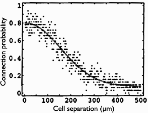
The position and connectivity of neurons in real neuronal systems is thought to be highly optimized to minimize the length of connecting fibres (Chen et al. 2006). At the level of individual neurons the connectivity pattern is so complex that only generalized statistics can be produced. These show that in the mouse cortex, for example, there are about 16 million neurons, each connected to about 8000 other neurons (Braitenberg and Schüz 1998). The density of the connectivity is impressive, with approximately a billion synapses in each cubic millimetre of cortex. Most of the connections are local, with the probability of any two neurons in the same area being connected, falling off in a Gaussian like manner (Hellwig 2000), see figure 1. It is thought extremely unlikely that these intra-area connections are highly structured as they are added at the rate of about 40,000 a second as the cortex matures. Cortical connectivity is of particular interest, as it is thought that one major function of the cortex is to act as a very large associative memory (Braitenberg and Schüz 1998).

Figure 1. The probability of a connection between any pair of neurons in layer 3 of the rat visual cortex against cell separation. Source: Hellwig, 2000, with permission.

2.5 Related work

Several researchers have investigated the standard sparse Hopfield network with small-world connection graphs (Bohland and Minai 2001, McGraw and Menzinger 2003, Morelli et al. 2004). Davey et al. also gave results for small-world networks of perceptrons (Davey et al. 2006). Other investigations have been reported in which sparse Hopfield networks are connected with scale-free connection graphs (for example da Fontoura Costa and Stauffer 2003, Kosinski and Sinolecka 1999, Perez Castillo et al. 2004, Stauffer et al. 2003 and Torres et al. 2004). Another approach is to build networks with a modular structure (see for example Horn et al. 1999, Renart et al. 1999). The present work differs from the foregoing in its focus on the efficiency of connection strategies, and in the range of connection architectures examined.

3. Network architecture

All networks discussed here are based on a one-dimensional lattice of N nodes with periodic boundary conditions. The networks are sparse, in which the input of each node is connected to a relatively small, but fixed number, k, of other nodes. The main networks examined here consist of either 500 or 5000 nodes, with 50 afferent (incoming) connections per node.

We are interested in comparing a number of different connection strategies to see which is the most efficient, both in terms of overall pattern completion ability and also in terms of economy of wiring. We compare five different wiring strategies.

3.1 Progressive rewiring

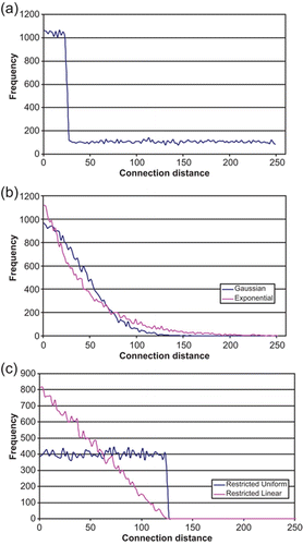
This is based on the strategy introduced by Watts and Strogatz (Watts and Strogatz 1998) for generating small-world networks; and was first applied to an associative memory by Bohland and Minai (Bohland and Minai 2001). A locally-connected network is set up, and a fraction of the afferent connections to each node is rewired to other randomly-selected nodes. Figure 2a shows the connectivity profile of a progressively-rewired network of 500 units, each with 50 afferent connections, at a setting of 50% rewiring. Rewiring in this way improves communication throughout the network, and it is found that as the degree of rewiring is increased, pattern completion progressively improves, up to the point where about half the connections have been rewired. Beyond this point, further rewiring seems to have little effect (Bohland and Minai 2001).

Figure 2. (a). Connectivity histogram for a progressively-rewired network at a setting of 50% rewiring, with a class interval of 2. The network consists of 500 units, each with 50 afferent connections per node; (b). Connectivity histogram for a Gaussian network at a σ of 40, and an exponential network at a λ of 0.025, with a class interval of 2. The networks consist of 500 units, each with 50 afferent connections per node; (c). Connectivity histogram for a restricted uniform and restricted linear network, each set to a connection limit of 50% of the maximum connection distance of the network (d _lim=125, d _max=250). The class interval is 2. The network consists of 500 units, each with 50 afferent connections per node.

3.2 Gaussian

Here the network is set up in such a way that the probability of a connection between any two nodes separated by a distance d around the ring is proportional to

where d is defined such that the distance between adjacent nodes is 1, and lies in the range 1≤d<N/2. Network performance is tested for a wide range of values of σ. Figure 2b shows the connectivity profile of a network of 500 units, each with 50 afferent connections, based on a Gaussian connectivity distribution with a σ of 40.

3.3 Exponential

In this case the network is set up in such a way that the probability of a connection between any two nodes separated by a distance, d, (where 1≤d<N/2) is proportional to

Networks are tested over a wide range of λ. Figure 2b shows the connectivity profile of a network of 500 units, each with 50 afferent connections, based on an exponential connectivity distribution with a λ of 0.025.

3.4 Restricted-uniform

With this particular architecture, no connections are permitted when the distance between two nodes exceeds a given limiting distance d _lim. At distances less than d _lim, all connections are of equal probability. Networks with a wide range of values of are used, where d _max is the maximum possible connection distance, equal in every case to N/2, where N is the number of nodes in the network (there are N/2 nodes either side of any given connection point around the ring). The reason for introducing this particular connection strategy is to examine the effect of eliminating all distal connections in a network. Figure 2c shows the connectivity profile of a network of 500 units, each with 50 afferent connections, based on a restricted-uniform connectivity distribution in which .

3.5 Restricted-linear

The rationale for introducing this network architecture is similar to that for the restricted uniform network mentioned above. There is again a connection distance d _lim beyond which the probability of connection is zero, but now the probability of connection for all distances up to d _lim is proportional to d _lim−d, where d is the distance between the two nodes under consideration. The connection profile for this architecture is again given in figure 2c, for a network of 500 units, each with 50 afferent connections, based on a restricted linear connectivity distribution in which . Networks are tested over a range of values of .

4. Results and Discussion

4.1 Gaussian, exponential and rewiring architectures compared

Our first experiment used a network of 5000 units with 50 afferent connections per node, set up with three different architectures – a progressively-rewired network with rewiring percentages ranging from 0 to 100, a family of Gaussian networks whose σ varied from 10 to 2500, and a set of exponential networks with λ in the range 0.001 to 0.06. In each case, the range of parameters was chosen to take the network from a locally-connected state at one extreme to a largely random state at the other. Values of EC were measured for each variant of each network type, and the results for the progressively-rewired and the Gaussian networks are shown in figure 3.

Figure 3. (a) (left). Effective Capacity vs. degree of rewiring. Rewiring beyond about 50% of connections yields little further advantage; (b) (right). Effective Capacity vs. Gaussian σ. Values of σ of 200 and above achieve an Effective Capacity equalling that of the random network. The networks consist of 5000 units, each with 50 afferent connections. Results are averages over 10 runs.

The progressively-rewired network exhibits a similar curve to that discovered by Bohland and Minai (2001), with a relatively poor performance when the network contains only local connections, and with performance progressively improving as the degree of rewiring increases. Once the degree of rewiring reaches about 50%, little further improvement occurs. At 100% rewiring, this is a random network, and its theoretical capacity is at a maximum.

As expected, the performance of the Gaussian and exponential architectures approaches that of the local network when the distributions are very tight (small σ or relatively large λ) and both achieve the same maximum EC of 23 as the random network, when the spread of connections is broad (large σ or relatively small λ).

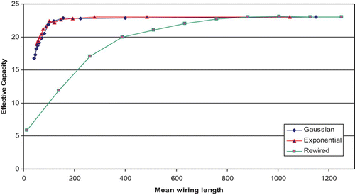
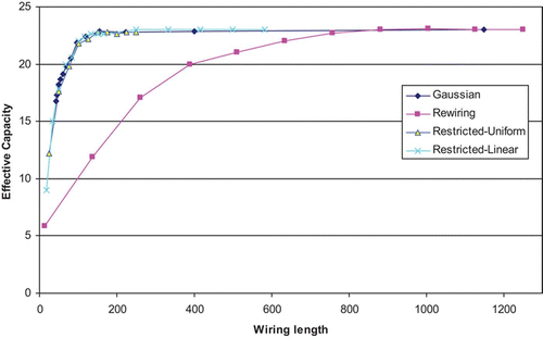
In order to facilitate more useful comparisons between the three networks and to highlight their pattern-completion performance at low mean wiring lengths, we use the data from the above simulations to plot the EC for each network variant against its corresponding mean wiring length. This immediately pays dividends: from figure 4 it is very clear that while all three networks are capable of achieving the same high values of EC, the Gaussian and exponential networks do so at considerably lower mean wiring lengths. In order to achieve an EC of 22, for example, the rewired network would need to be 50% rewired and this results in a mean wiring length of 630, whereas the Gaussian (at a σ of 120) and the exponential network (at a λ of 0.01) would both have a mean wiring length of just 96, and are thus considerably more efficient in terms of achieving high EC at low mean wiring length.

Figure 4. Effective Capacity against mean wiring length for a network of 5000 units with 50 afferent connections per node (connectivity level, k/N, of 0.01). Comparison of Gaussian, exponential and rewiring architectures. Results are averages over 10 runs for each network setting.

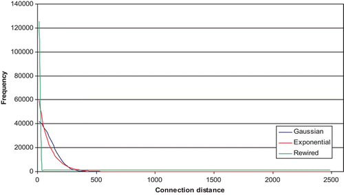
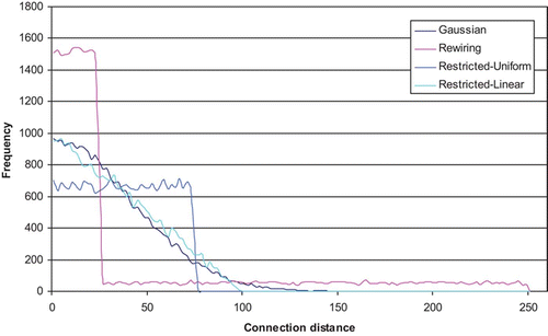
The high mean wiring length of the progressively-rewired network is caused by the relatively large number of distal connections, which occur as the network is rewired. From the relatively good performance of the Gaussian and exponential distributions, however, it is clear that not all of these distal connections are essential for good pattern-completion performance. Just how few are needed becomes clear from histograms showing connectivity profiles for the three network variants at the point where the EC is 22 (at a σ of 120, a λ of 0.01 and at a rewiring of 50%; see figure 5). It is immediately clear that the Gaussian and exponential distributions have few if any distal connections, and yet achieve excellent pattern-completion performance. They achieve this by relaxing the constraint of strictly local connectivity in favour of a broader, but still reasonably local distribution of connections.

Figure 5. Connectivity histogram for a network of 5000 units, each with 50 connections (connectivity level, k/N, of 0.01), comparing Gaussian, exponential and rewiring architectures with the same relatively high Effective Capacity of 22. The class interval is 25.

We should also note the closeness of the Gaussian and exponential curves in figure 5. It would seem that the small differences between these two distributions are of little importance, when designing a high performance architecture for a sparse auto-associator.

4.2 Exploring architectures with restricted maximum connection lengths

The good performance of the Gaussian and exponential distributions, as evidenced above, seems to imply that a large number of distal connections are not essential for good pattern-completion in a sparse associative network. In order to see if they are necessary at all, we looked at the performance of two networks in which the maximum connection distance can be controlled – the restricted-uniform and restricted-linear architectures described above, and depicted in figure 2c.

Using a network of 5000 units, each with 50 afferent connections, we took measurements of EC for these two new network architectures, as the maximum permitted connection distance was progressively increased from around 10% to 100% of the total connection distance afforded by the network. As with the previous experiment, we ploted the EC of each variant of each network type against the mean wiring length of the corresponding networks. The results appear in figure 6, alongside those of the Gaussian and the progressively-rewired network. To improve clarity, the results for the exponential architecture have not been plotted here since they are indistinguishable from those of the Gaussian. It can be seen immediately from this graph that the performance of both the restricted-uniform and restricted-linear networks closely track that of the Gaussian. Yet, these two distributions have no distal connections whatsoever.

Figure 6. Effective Capacity against wiring length for a network of 5000 units, each with 50 afferent connections (connectivity level, k/N, of 0.01). Plots are shown for the Gaussian architecture, the progressively-rewired architecture and the restricted-uniform and restricted-linear architectures. Results are averages over 10 runs for each network setting.

This demonstrates at a stroke that in order to achieve a high EC at low mean wiring length in a sparsely-connected network, there is no need for the presence of any distal connections whatsoever. From this perspective, the asymptotic tails of the Gaussian and of the exponential appear to be redundant.

4.3 Comparing networks with higher connectivity levels

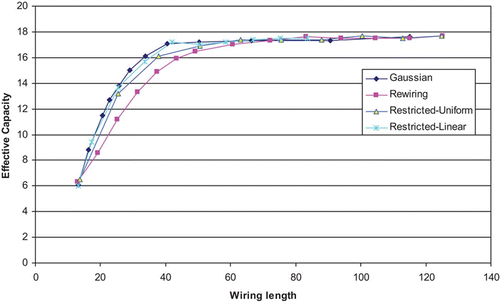
In networks with higher levels of connectivity, the difference in performance between the different architectures is much less marked. Figure 7 shows a similar plot of EC against wiring length to that of figure 6, but for a network of 500 units, each with 50 afferent connections – ten times the connectivity level of the previous networks. To improve clarity, the results for the exponential architecture have again been omitted since they are indistinguishable from those of the Gaussian. The first thing to emerge from this graph is that the progressively-rewired network again performs the worst, but that it is now much closer to the others. On the other hand, it appears as if there is now a marginal difference between the restricted-uniform and the better-performing Gaussian. The performance of the restricted-linear architecture is again indistinguishable from that of the Gaussian.

Figure 7. Effective Capacity against wiring length for a network of 500 units, each with 50 afferent connections (connectivity level, k/N, is 0.1). Plots are shown for the Gaussian architecture, the progressively-rewired architecture and the restricted-uniform and restricted-linear architectures. Results are averages over 50 runs for each network setting.

Figure 8 shows the profiles of the four networks under discussion at settings, which give rise to comparable values of EC close to 16 (16.1 on the Gaussian network, at σ=42; 15.9 on the progressively-rewired network, at 25% rewiring; 16.1 on the restricted-uniform network, at a length restriction of 30% of the maximum possible connection length and 15.7 on the restricted-linear network, at a length restriction of 40% of the maximum connection length). These points have corresponding mean wiring lengths of 33.8, 43.3, 38.0 and 33.7, respectively. The close similarity of the Gaussian and the restricted-linear profiles here makes it clear why these two networks share the same pattern-completion performance. And it is perhaps surprising, in view of the obvious differences between the restricted-uniform profile and that of the Gaussian, that the former performs so well.

Figure 8. Connectivity histogram for a network of 500 units, each with 50 afferent connections (connectivity level, k/N, is 0.1), comparing the four architectures at the point where Effective Capacity is close to 16 – Gaussian, progressively-rewired, restricted-uniform and restricted-linear. The class interval is 2.

To summarize our results to this point, it emerges that when designing sparsely-connected networks to be used as associative memories, and where good pattern completion performance with randomly generated patterns is required at low wiring costs, progressively-rewired networks perform poorly. They achieve the same EC as other network architectures, but they do so at relatively high wiring costs. These relative costs increase when the network becomes more sparse. By contrast, relatively tight Gaussian, exponential and restricted-uniform and -linear architectures perform well, achieving high ECs at low wiring costs.

The high EC achieved by relatively tight connectivity distributions appears to suggest that direct long distance communication across the network is not essential for good pattern completion performance. To further underline this point there appears to be no significant difference in performance between the Gaussian and restricted-linear architectures, even in the more demanding sparser network – the Gaussian's asymptotic tail, which would give better communication across the network than the restricted-linear distribution in which no distal connections are permitted, is redundant.

4.4 Optimal Gaussian distributions

In the foregoing we have studied a number of different architectures using networks of size 500 and 5000 units. Both networks had 50 afferent connections per node, giving us connectivity levels, k/N, of 0.1 and 0.01, respectively. From a comparison of figures 5 and 8, we can see that in the sparser of the two networks (figure 5), we could use relatively tighter Gaussian or exponential distributions (i.e. relative to network size) without significantly impairing performance. In the sparser network a σ of around 5% of the maximum connection length of the network gave good results, whereas in the less sparse network, a σ of around 15–20% of the maximum connection length was needed.

The question naturally arises: to what extent does the connectivity profile of the best performing networks depend on network size and connection density? To establish an answer to this question, we first measured the performance of a network with Gaussian connectivity distribution with a fixed value of σ set to 120 (known to give good performance) and another set to 30 (giving a performance intermediate between that of a local and a random network). The networks were tested under conditions of increasing network size, but with the number of connections per node remaining fixed at 50. We, then, repeated this procedure for locally-connected and random networks of the same configuration.

Figure 9 shows the interesting results. From this it may be seen that all four networks exhibit a largely constant value of EC, as the size of the network is increased from 1000 to 10,000 units. Clearly network size per se, does not influence EC within this range of network sizes; and a Gaussian network with a given value of σ achieves the same EC regardless of network size. This occurs because the effect of the increase in the network size, N, is automatically offset by the concomitant increase in the number of bits per pattern (since in a generic Hopfield network the number of bits per pattern is simply equal to the total number of nodes in the network).

Figure 9. Effective Capacity vs. network size for a network with a fixed number of connections per node, k (=50), for four different connection strategies – a locally-connected network, a random network and ones with Gaussian connectivity distributions with a σ of 30 and with 120 – averages over 10 runs.

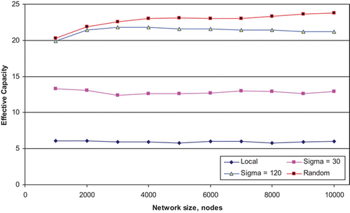
What is unexpected here is that with the value of σ for the connectivity distribution of the network held constant as the network increases in size, there is no deterioration in performance. Clearly, as the network becomes larger and larger, there is no need to broaden the Gaussian connectivity distribution in order to maintain the EC of the network. In many networks, the characteristic path length (the average over the whole network of the shortest path linking each pair of nodes) is known to have important implications for the rate at which information can move through a network. For example, in network models of the spread of disease, the time taken for the whole population to be infected is related to the characteristic path length (Watts and Strogatz 1998). However, in our sparsely-connected network with a Gaussian connectivity profile of σ=30, we find that the network continues to perform at the same level (with an EC of about 13) as the network size is increased from 1000 units to 10,000 units. During this time the measured degree of clustering remains fixed at about 0.5, but the mean minimum path length increases from about 4 to around 20. Clearly the mean minimum path length is not a factor that appears to have any bearing on the pattern-completion performance of this network.

In a second experiment we held the network size constant, at 5000 units, but gradually increased the number of connections per node from 50 to 500. This procedure was used initially with four different connection strategies – local and random connectivity, a local network with 10% of connections rewired to random nodes and a Gaussian connectivity distribution with a fixed σ of 30.

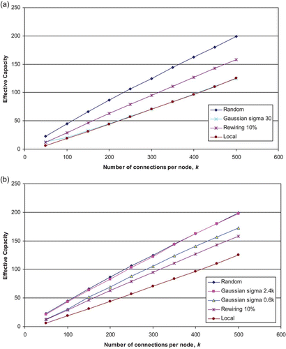
As may be seen from Figure 10a, the networks with local connectivity, random connectivity and with 10% rewiring show a linear relationship between EC and the number of connections per node. This suggests, as we have previously argued (Calcraft et al. 2006), that for large networks the EC is directly proportional to the underlying maximum theoretical capacity of the network (since the theoretical capacity of such networks is itself proportional to k (Hertz et al. 1991)). Of the plots depicted, the locally-connected network performs the worst, and the random network, the best. The Gaussian network with a constant value of σ initially performs as well as the 10% rewired network, but as soon as the number of connections per node is increased from its starting value of 50 to 100, relative performance drops, and from then on its Effective Capacity tracks that of the locally-connected network. Clearly as the number of connections per node of a network increases, σ must also be increased if relative performance is not to deteriorate.

Figure 10. (a) Effective Capacity vs. the number of connections per node in a fixed-size network of 5000 units, showing the effect of using different connection strategies – random and local connectivity, a local network with 10% of connections rewired to random nodes and a Gaussian connectivity distribution with a fixed σ of 30. Results are averages over four runs; (b) Effective Capacity vs the number of connections per node in a fixed-size network of 5000 units, showing the effect of using different connection strategies: Random and local connectivity, a local network with 10% of connections rewired to random nodes, and two Gaussian connectivity distributions whose value of σ is made proportional to k, the number of connections per node (in one case σ is set to 2.4 k and in the other to 0.6 k). Results are averages over four runs.

This suggests that we need to increase the value of σ in the Gaussian distributions when we increase k. Figure 10b demonstrates the effect of this, depicting the performance of two Gaussian connectivity distributions whose values of σ were made proportional to k, the number of connections per node. For these two plots we have made σ equal to 0.6 k, and to 2.4 k, factors chosen to give values of σ of 30 and 120, respectively, when k is 50, as used in the experiments above. As can be seen, the performance of these two networks does not drop with increasing k, but instead increases linearly with k in a similar way to that of the other three non-Gaussian networks. The network whose value of σ is set to 0.6 k exhibits a slope slightly greater than that of the 10% rewired network, whereas that with a σ of 2.4 k tracks the response of the random network very closely indeed. The important result thus emerges that by making σ proportional to the number of connections per node in a sparse network, we obtain consistent performance, as the network is scaled up or down in size.

4.5 Scaling effects

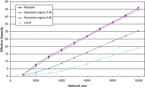
In the above, we have examined the way that different networks behave when either the number of units or the number of connections per unit is increased. We did this to establish the relationship between network size and Gaussian σ for well-performing networks, when relatively small network sizes were used. We now turn our attention to a different though related question: how well do the networks studied here scale up – does the performance of the networks continue to increase linearly as the network is scaled up in size? To answer this question we have run two simulations, one using a connectivity level, k/N, of 0.01 and the other with 0.1. In both cases, measurements of EC were made as the networks were progressively increased in size, while keeping the connectivity level, k/N, at a constant 0.01 or 0.1. In the network with connectivity level 0.1 three different architectures were used – local connectivity, random connectivity and a Gaussian connectivity distribution in which σ was maintained at a value of 0.8 k, where k is the number of connections per node. This value gives a σ of 40 when k=50, and thus corresponds to the well-performing configuration examined earlier with the 0.1 connectivity network. In the case of the 0.01 connectivity network we have used Gaussian architectures with a σ of 0.6 k and 2.4 k, as previously explored, alongside random and local networks.

The results appear in figure 11 for a fixed connectivity level, k/N, of 0.1, and in figure 12 for a connectivity level of 0.01. The first point to note from both graphs is their extreme linearity. The only departure from this is in the sparser of the two networks at the left-hand side of the plot, where the number of connections per node, and thus the resultant EC, is very low. Once the EC exceeds a value of 4 or 5, all architectures exhibit a highly linear relationship between EC and network size.

Figure 11. Effective Capacity of networks based on different connection strategies, as network size is increased from 1000, while keeping a fixed connectivity level, k/N, of 0.1. The results are averages over four runs.

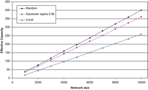
Figure 12. Effective Capacity of networks based on different connection strategies, as network size is increased from 1000, while keeping a fixed connectivity level, k/N, of 0.01. The results are averages over four runs.

We have previously claimed (Calcraft et al. 2006) that in large networks, whether fully or sparsely-connected, EC is proportional to the underlying capacity of the network (which is itself proportional to k, the number of connections per node in a sparsely-connected network), and the linearity of these plots strongly supports this view. It can further be seen that the slope of each line is dependent on the architecture. And since no architecture has a lower theoretical capacity than a locally-connected network, and none has a higher capacity than a random network, we would expect to find that all other conceivable architectures would result in lines contained within the bounds formed by the local and random plots.

Since the EC of the architectures tested appears to increase linearly with increasing network size (beyond initial size effects), it seems reasonable to suppose that this linearity will continue, as the network expands still further – a fact which we have confirmed by taking spot measurements at much larger network sizes (50,000 units for the 0.01 connectivity level network and 20,000 units for the network with 0.1 connectivity level). The general findings of this paper thus appear to be robust for networks of considerable size, and indeed we see no reason why these networks should not scale to sizes well beyond the scope of current day technology.

4.6 Convergence times

Our results suggest that when trying to achieve good pattern-completion performance at low mean wiring lengths in sparsely-connected networks, it is desirable to use only relatively short-range connections. Long-range connections appear not to be necessary when achieving good pattern completion with randomly generated patterns, and to be positively detrimental when wiring costs are taken into account. However, this analysis currently makes no reference to the convergence time of the network – the number of cycles which the recurrent network takes when moving towards a fundamental memory of the network as it progressively ‘repairs’ a damaged pattern. It might reasonably be expected that the presence of a significant number of distal connections in a sparse network would be an important factor in keeping convergence times for the network to a minimum, since their presence would improve the effective speed of communication across the network. Our final experiment is designed to test this supposition.

Convergence times are not simply an intrinsic property of a given network. They will critically depend upon the degree of difficulty of the task that the network is required to perform – the degree of difference between a presented pattern and the closest fundamental, or indeed spurious memory. The further the ‘distance’ between these two, the longer the convergence time. In order to explore the effect of using different connectivity strategies on convergence times we have taken measurements of convergence times in our networks, as increasing levels of noise are applied to the pattern set, progressively increasing the degree of difficulty of the task.

When measuring EC, we are attempting to see how many patterns (damaged by applying 60% noise) the network can on an average reinstate to within 95% of the original. In the following tests we have measured convergence time as we applied increasing levels of random noise, from 4% to greater than 60%. The point at which the noise is 60% corresponds to the exact conditions of the EC measurement for the three networks.

We have performed these measurements for both 500 and the 5000 unit networks, both of which have 50 afferent connections per node. In the case of the smaller network we have used parameter settings of the various architectures, which result in an EC of 16 (a value close to the maximum of 17, but where wiring lengths are kept to a minimum). We have trained the networks on 16 patterns, and measured convergence times on recall for different levels of noise applied to the test pattern set. In the case of the larger network, we used a similar approach, though the networks were trained on 20 patterns (again, a value close to the maximum of 23, but where wiring lengths are low), matching the quantity of patterns successfully learned during earlier EC tests. The results appear in figures 13 and 14.

Figure 13. Convergence time (measured in cycles) vs. the degree of noise applied to each pattern in a network of 500 nodes, each with 50 afferent connections. A range of architectures is represented, each of whose parameters gives rise to an Effective Capacity of 16. Each network is trained on 16 patterns, thus the point at which the noise is 60% corresponds to the exact conditions of earlier Effective Capacity measurements. Results are averages over 50 runs.

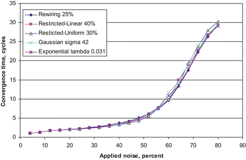
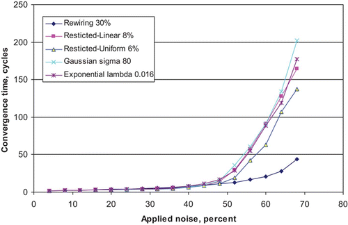
Figure 14. Convergence time (measured in cycles) vs. the degree of noise applied to each pattern in a network of 5000 nodes, each with 50 afferent connections. A range of architectures is represented, each of whose parameters gives rise to an Effective Capacity of 20. Each network is trained on 20 patterns, thus the point at which the noise is 60% corresponds to the exact conditions of earlier Effective Capacity measurements. Results are averages over 10 runs.

In the case of the smaller network (figure 13), all architectures perform in exactly the same way, with convergence times increasing at a relatively slow rate until the applied noise reaches about 45%, and the convergence time is around four or five cycles. Convergence times then increase relatively sharply, reaching more than 25 cycles when the noise reaches 75%.

In the larger sparser network (figure 14), convergence times again increase relatively slowly until the noise reaches around 45%, where convergence time is now around 10 cycles. After this point, all but the randomly-rewired network show reasonably steep increases in convergence time, reaching significantly higher levels than the 500 unit network. For example, the restricted-uniform architecture in the 5000 unit network has a convergence time of 140 cycles at a noise level of 68%, whereas in the 500 unit network, convergence time was only at around 17 cycles for the same amount of noise.

Thus, we see that there is a price to be paid for adopting more efficient patterns of connectivity over the random network. However, the relative increase in convergence time observed only occurs in the sparser of the two networks examined – that with a connectivity level, k/N, of 0.01. Furthermore, the difference only appears when the networks are working under extreme conditions. At the current pattern loadings, if the noise applied to the pattern set is kept below 50%, there is no discernible difference between convergence times of any of the network architectures, even when the connectivity level is only 0.01.

Thus, when searching for the most efficient pattern of connectivity for a sparsely-connected associative memory, where good pattern-completion performance on random patterns is required at low wiring costs, networks based on Gaussian, exponential, restricted-uniform or restricted-linear architectures can safely be used without any issues of increased convergence times, except in the case of very sparse heavily loaded networks, where randomly-rewired networks have lower convergence times, albeit at the cost of significantly greater mean wiring length.

5. Conclusions

In the foregoing, we have examined the pattern-completion performance of sparsely-connected associative memory models, built using a number of different connection strategies. Networks based on progressively-rewired, Gaussian, exponential, restricted-uniform and restricted-linear architectures were tested at network sizes of 500 and 5000 units, each with 50 afferent connections per node.

It was found that all five architectures were capable of achieving the same best pattern-completion results, at particular settings of their parameters. For example, the Gaussian needed a large value of σ, giving a broad connectivity distribution, and the progressively-rewired network needed to be rewired by at least 40% or 50%. But when the mean wiring length of the networks was taken into account, major differences emerged. The poorest performer was the progressively-rewired network, based on the strategy originally proposed by Watts and Strogatz (1998). In the sparser of the two networks under test (with 5000 units, each with 50 connections, yielding a connectivity level, k/N, of 0.01), the mean wiring length of the progressively-rewired network was as much as six times that of its Gaussian counterpart. In the 500 unit network, with 0.1 connectivity level, the performance of the rewired network came closer to that of the Gaussian, but was still markedly poorer.

In both the 500 and the 5000 unit networks, the Gaussian and exponential architectures consistently achieved some of the best results, when wiring costs were taken into account. In the sparser of the two networks, very good pattern completion results were obtained with relatively tight Gaussian profiles in which a σ of just 120 was used in a network whose maximum connection distance was 2500. This suggested that in such sparse networks, very few, if any, distal connections are needed in order to maintain good pattern-completion for randomly generated patterns. In the 500 unit network, the Gaussian σ needed to be relatively larger (i.e. compared with the size of the network) in order to achieve equivalent performance.

We introduced the restricted-linear architecture in order to determine to what extent the asymptotic tail of the Gaussian, with its small number of relatively long-distance connections, was necessary in order to maintain good communication across the network, and achieve good pattern-completion. It was clear in both the 5000 unit and the 500 unit networks that the performance of the restricted-linear architecture was indistinguishable from that of the Gaussian, and we thus concluded that from the point of view of achieving good pattern completion using randomly generated patterns at low mean wiring length, there is no need for distal connections whatsoever. Clearly, connections should not be entirely local, since local networks always perform badly, but connections should, however, all be located relatively close to the host node, and it would seem that the precise distribution shape is not critical, and becomes even less so in sparser networks.

Our experiments showed that in networks with a constant connectivity level k/N, the optimum width of the Gaussian connectivity distributions relative to the size of the network changed as network size was increased, and we set out to determine what factors affected this. We obtained the interesting result that in order to maintain the relative performance of a network based on a Gaussian connectivity distribution, Gaussian σ needs to be made proportional to k, the number of connections per node. This is robust for networks with increasing k or with increasing k and N.

It was considered that by adopting a Gaussian or similar architecture with a tight connectivity distribution in order to obtain good pattern-completion performance at low wiring costs, there might be a risk that the resultant impairment of communication across the network could also result in an unwanted increase in convergence times. Tests were therefore carried out with both the 500 and 5000 unit networks, and it was found that the only noticeable impairment occurred in the sparser of the two networks, and only at the point where the networks were most heavily stressed. When trained on 20 patterns, and with 60% of random noise applied to each pattern, convergence times of the Gaussian and other networks rose sharply, while that of the progressively rewired network (rewired by 30%) showed a slower rise. However, this effect was not noticeable at noise levels below 50%. Thus, it would appear that only in very sparse and highly stressed networks is there any advantage in using a progressively-rewired connectivity distribution, with its high wiring costs, over the much more efficient Gaussian, exponential, restricted-uniform or restricted-linear architectures.

To complete our study, we considered to what extent our results would also apply to much larger networks. To this end we studied the Effective Capacity of networks built using a number of different architectures. Measurements were taken as the networks were scaled up, all the time maintaining a constant connectivity level, k/N.

Beyond initial size effects, all networks exhibited a highly linear performance, in the full range of experiments up to network sizes of 10,000 units. Further spot measurements were made at network sizes of 20,000 units for the networks with 0.1 connectivity level, and at 50,000 units for the 0.01 connectivity level networks, and these again confirmed the extreme linearity of the Effective Capacity measure for the range of different architectures as network size is increased. We thus conclude that our findings, in terms of network architecture and performance, are applicable in the range of networks accessible to current technology.

References

- Bohland , J. and Minai , A. 2001 . Efficient Associative Memory Using Small-World Architecture . Neurocomputing , : 489 – 496 . 38–40
- Braitenberg , V. and Schüz , A. 1998 . Cortex: Statistics and Geometry of Neuronal Connectivity , Berlin : Springer-Verlag .
- Buzsaki , G. , Geisler , C. , Henze , D. A. and Wang , X.-J. 2004 . Interneuron Diversity series: Circuit complexity and axon wiring economy of cortical interneurons . Trends Neurosci. , 27 : 186
- Calcraft , L. 2005 . Measuring the Performance of Associative Memories . Report Number 420 University of Hertfordshire
- Calcraft , L. , Adams , R. and Davey , N. 2006 . Locally-connected and small-world associative memories in large networks . Neural Information Processing - Letters and Reviews , 10 : 19 – 26 .
- Chen , B. L. , Hall , D. H. and Chklovskii , D. B. 2006 . Wiring optimization can relate neuronal structure and function . Proc. Natl. Acad. Sci. , 103 : 4723 – 4728 .
- da Fontoura Costa , L. and Stauffer , D. 2003 . Associative recall in non-randomly diluted neuronal networks . Physica A: Stat. Mech. Appl. , 330 : 37
- Davey , N. , Calcraft , L. and Adams , R. 2006 . High capacity, small-world associative memory models . Connect. Sci. , 18 : 247
- Hellwig , B. 2000 . A quantitative analysis of the local connectivity between pyramidal neurons in layers 2/3 of the rat visual cortex . Biol. Cybern. , 82 : 111
- Hertz , J. , Krogh , A. and Palmer , R. G. 1991 . Introduction to the Theory of Neural Computation , Redwood City, CA : Addison-Wesley Publishing Company .
- Horn , D. , Levy , N. and Ruppin , E. 1999 . Associative Memory in a Multimodular Network . Neural Comput. , 11 : 1717 – 1737 .
- Kosinski , R. A. and Sinolecka , M. M. 1999 . Memory Properties of Artificial Neural Networks with different types of dilutions and damages . Acta Phsica Polonica B , 30 : 2589 – 2594 .
- McGraw , P. and Menzinger , M. 2003 . Topology and computational performance of attractor neural networks . Phys. Rev. E , 68 : 047102
- Morelli , L. G. , Abramson , G. and Kuperman , M. N. 2004 . Associative Memory on a small-world neural network . Eur. Phys. J. B , 38 : 495 – 500 . 2004
- Perez Castillo , I. , Wemmenhove , B. , Hatchett , J. P.L. , Coolen , A. C.C. , Skantzos , N. S. and Nikoletopoulos , T. 2004 . Analytic solution of attractor neural networks on scale-free graphs . J. Physics A, Math. Gen. , 37 : 8789
- Renart , A. , Parga , N. and Rolls , E. T. 1999 . Associative memory properties of multiple cortical modules . Netw., Comput. Neural Syst. , 10 : 237 – 255 .
- Stauffer , D. , Aharony , A. , da Fontoura Costa , L. and Adler , J. 2003 . Efficient Hopfield pattern recognition on a scale-free neural network . Eur. Phys. J.B , 32 : 395 – 399 .
- Torres , J. J. , Munoz , M. A. , Marro , J. and Garrido , P. L. 2004 . Influence of topology on the performance of a neural network . Neurocomputing , : 229 – 234 . 58–60
- Watts , D. and Strogatz , S. 1998 . Collective Dynamics of ‘small-world’ networks . Nature , 393 : 440 – 442 .