Support-vector-based emergent self-organising approach for emotional understanding

Abstract

This study discusses the computational analysis of general emotion understanding from questionnaires methodology. The questionnaires method approaches the subject by investigating the real experience that accompanied the emotions, whereas the other laboratory approaches are generally associated with exaggerated elements. We adopted a connectionist model called support-vector-based emergent self-organising map (SVESOM) to analyse the emotion profiling from the questionnaires method. The SVESOM first identifies the important variables by giving discriminative features with high ranking. The classifier then performs the classification based on the selected features. Experimental results show that the top rank features are in line with the work of Scherer and Wallbott [(1994), ‘Evidence for Universality and Cultural Variation of Differential Emotion Response Patterning’, Journal of Personality and Social Psychology, 66, 310–328], which approached the emotions physiologically. While the performance measures show that using the full features for classifications can degrade the performance, the selected features provide superior results in terms of accuracy and generalisation.

Keywords:

• self-organisation map
• support-vector machine
• emotion

1. Introduction

Emotion is a complicated aspect of the human inner state. The ability to understand, interpret and react to emotions is vital in maintaining relationships with friends, colleagues and family (Ekman 2004; Levine 2007; Perlovsky 2007). The brain, which is the most fundamental source of emotion, exhibits an alpha rhythm that can be detected by Electro-Encephalogram (EEG) (Sears and Jacko 2008). The electrical activity, produced by firing of neurons within the brain, is recorded along the scalp. EEG studies (Davidson, Schwartz, Saron, Bennett, and Goleman 1979) have shown that positive emotions lead to greater activation on the left anterior region of the brain, while negative emotions lead to more significant activation on the right anterior region. Recent advances in functional Magneto Resonance Imaging (fMRI) provide more sophisticated monitoring of emotion (Phan, Wager, and Taylor 2002; Desseilles et al. 2006; Westen, Blagov, Harenski, Kilts, and Hamann 2006; Redcay et al. 2010).

Apart from brain measurements for monitoring human emotion, another area of emotion research is emotion recognition. The research of emotion recognition has been found in many published works, which are mainly focusing on facial expressions recognition since facial expressions represent a straightforward means of expressions. The first known facial expression analysis was presented by Darwin in 1872 (Darwin 1872). The article presented the universality of human face expressions and the continuity in man and animals. It was also pointed out that there are specific inborn emotions, which originated in serviceable associated habits. After almost a century, Ekman and Friesen (1971) postulated six primary emotions that possess a distinctive content together with a unique facial expression. These prototypical emotional displays are referred to as basic emotions in many of the later literature. The six universally recognised emotions are joy, sad, fear, disgust, surprise and anger. They further developed the facial action coding system (FACS) for describing facial expressions. FACS uses 44 action units (Aus) for the description of facial actions with regard to their locations as well as their intensity.

Another means of emotion recognition is through voice (Ververidis and Kotropoulos 2006). Voice can provide indications of valence and specific emotions through acoustic properties such as pitch range, rhythm, amplitude or duration changes (Ball and Breese 2000). A bored or sad user would typically exhibit slower, lower-pitched speech, with little high-frequency energy. A person experiencing fear, anger or joy would speak faster and louder, with strong high-frequency energy (Picard 1997). The database of speech recognition generally consists of recorded speech synthesis, prosodic modelling, speech conversion that are voiced out by actors like the work in Lutfi, Montero, Barra-Chicote, Lucas-Cuesta, and Ascensión (2009).

Both face and speech emotion recognition are laboratory approaches that mandates the use of databases with directed facial expressions or acted tones to provide training for the recognition systems. The emotions are, however, typically exaggerated and rarely appear in the real world. It is difficult to study emotional experiences by using laboratory techniques of emotion induction or field observation. Emotion induction in the laboratory is often inefficient as it results in weak emotional experience due to the fact that strong emotions are difficult to undertake in real-life situations outside the laboratory. This leads to the third category of emotion recognition and profiling, called the questionnaire approach. In the questionnaire approach, the subjects are given a set of questions to help them recall occasions which they have experienced with different emotions. This is a self-reported measurement to measure the affective states. Although it can be argued that questionnaires are only capable of measuring conscious experience of emotion, and most of the affective processes are non-conscious processes (Wallbott and Scherer 1985), this approach represents the most direct way to measure sentiment. The reason for adopting the questionnaires approach is that the questionnaire is not artificially generated because it is naturally based on the recalling of personal encounters. The questionnaire approach to studying emotional processes by asking subjects to describe emotional situations and the reactions experienced is a suitable way to study not only emotion-eliciting situations but also emotional reactions. Scherer and Wallbott (1994) argued that the questionnaire approach to emotion study is preferable because it has access to real, intimate emotions through verbal report of recalled emotion experiences. Moreover, the two important components of the total emotion process, i.e. cognitive appraisal of emotion-antecedent situations and subjective feeling state are only accessible through self-reporting.

In this paper, we present a computational analysis for human emotions profiling based on the questionnaires approach. We make use of studies carried out by a group of psychologists directed by Scherer and Wallbott (see their studies in detail in Wallbott and Scherer 1988; Scherer and Wallbott 1994; Scherer 1997) in which they collected cross-cultural differences in the reaction patterns for seven emotions over 10 years. Such studies were presented in the International Survey on Emotion Antecedents and Reactions (ISEAR). The studies initially collected data from subjects living in eight European countries, Japan and the USA. They subsequently evolved to include close to 3000 respondents from 38 countries that cover the five continents. Student respondents, psychologists and non-psychologists were asked to report situations in which they had experienced all of seven major emotions (joy, fear, anger, sadness, disgust, shame, and guilt). As the database is too huge to be analysed, we need to design a robust classification method which is able to visualise and classify the characteristics of the questionnaires data simultaneously. Therefore, a new connectionist model is developed to visualise and classify data collected using the questionnaires approach. A benefit of this model over other techniques is its capacity to handle imbalanced data sets (IDS). The model adopts a derivation of support-vector machines (SVM) in selecting variables so that the problem of imbalanced data distribution can be relaxed (Nguwi and Cho 2009). Then, we used an emergent self-organising map (ESOM) to cluster the ranked features so as to provide clusters for unsupervised classification. The details of this model as well as its performance in analysing this questionnaires approach will be described in the rest of this paper.

The paper is organised as follows: Section 2 discusses the methodology of using support-vector-based emergent self-organising map (SVESOM) model to profile the emotions from the questionnaire approach. We first study the structure of questionnaire approach and then discuss the algorithm of the SVESOM in the same section. Section 3 presents the experimental results and discussion for the proposed method. Several validations have been conducted to present the performance of the proposed method. Finally, the conclusion of this paper is drawn in Section 4.

2. Emotional profiling through SVESOM

In our study, we refer to the research of Scherer and Wallbott (1994) which extrapolated from reported predictions on the basis of individual expressive behaviour variables. Basically, the questionnaires consist of four parts: (a) situation description; (b) subjective feeling state; (c) physiological symptoms, expressive behaviour and other reactions; and (d) appraisal. Table 1 illustrates the predictions of emotions in accordance to different subjective feelings, physiological symptoms and expressive behaviours together with the related variables and interpretations from ISEAR questionnaire. For the subjective feeling domain, predictions were made for the dimensions of intensity and duration of the affective state, which attempts at controlling the state, and how long ago the event took place. The physiological symptoms report individual reactions or symptoms that they recall. Cardiovascular, muscle symptoms and perspiration predictions were translated into ergotropic arousal predictions. Stomach symptoms, lump in throat and crying predictions were interpreted in terms of trophotropic arousal. Similarly, the expressive behaviour variables were grouped into movement, nonverbal-nonvocal, paralinguistic and speech behaviour (Scherer and Wallbott 1994).

Table 1. Predictions of emotions in accordance to different subjective feelings, physiological symptoms and expressive behaviours together with the corresponding variables and interpretation.

Measure	Prediction	Variable	Interpretation
Subjective feeling
Time distance (long ago–recent)	Sad = Fear<Joy = Anger	WHEN	When did this happen?
Intensity (weak–strong)	Anger = Fear<Sad = Joy	INTS	How intense was this feeling?
Duration (short–long)	Fear<Anger<Joy = Sad	LONG	How long did you feel the emotion?
Control attempts (weak–strong)	Joy<Fear = Sad = Anger	CON	Did subject try to control the feeling?
Physiological symptoms
Ergotropic arousal (weak–strong)	Sad = Joy<Anger<Fear	ERGO	Ergotropic arousal
Trophotropic arousal (weak–strong)	Joy<Fear = Anger<Sad	TROPHO	Trophotropic arousal
Felt temperature (cold–warm)	Fear<Sad<Joy<Anger	TEMPER	Felt temperature
Expressive behaviours
Approach/withdrawal (away–towards)	Fear = Sad = Anger<Joy	MOVE	Movement behaviour (move towards people?)
		EXP10	Moving against people or things
Non-verbal behaviour (little–much)	Fear<Sad<Joy = Anger	EXPRES	Non-verbal activity (laughing/crying and etc.)
		EXP1	Laughing, smiling
		EXP2	Crying, sobbing
Paralinguistic behaviours (little–much)	No predictions available	PARAL	Paralinguistic activity
Verbal behaviour (little–much)	Fear = Sad<Joy = Anger	VERBAL	Verbal activity (silence/lengthy utterance)
Notes: ‘<’ Indicates significant difference will be found between groups of emotions at either side of the sign; ‘=’ indicates no significant differences are expected.

Forty variables are extracted from the questionnaires using different questions as shown in Table 2. With the huge database (i.e. over 10,000 records), it is difficult to classify, as the classifiers may not be able to handle the overwhelming amount of data. The difficulty in classification arises from the fact that the distributions of data set are imbalanced. Based on the principle of Occam's razor (Thorburn 1915), classifiers generally do not perform well on IDS because they are designed to generalise from the limited numbers of sampling data and provide the simplest hypothesis that best fits to the data. IDS is a phenomenon that occurs where the number of instances in one class significantly outnumbered the instances from other classes. Therefore, the training data are dominated by the instances belonging to one class. We thereby introduce an approach which is derived from SVM that can actively select the appropriate variables according to the different emotions.

Table 2. Variables and interpretation from ISEAR questionnaire.

Var	Interpretations
RELI	Subject's religion
PRAC	Subject practicing religion
FOCC	Father's occupation
MOCC	Mother's occupation
FIEL	Subject's field of study
WHEN	When did this happen?
LONG	How long did you feel the emotion?
INTS	How intense was this feeling?
ERGO	Ergotropic arousal
TROPHO	Trophotropic arousal
TEMPER	Felt temperature
EXPRES	Non-verbal activity (laughing/crying and etc)
MOVE	Movement behaviour (move towards people?)
EXP1	Laughing, smiling
EXP2	Crying, sobbing
EXP10	Moving against people or things
PARAL	Paralinguistic activity
CON	Did subject try to control the feeling?
EXPC	Did subject expect the situation to occur?
PLEA	The event is pleasant or unpleasant?
PLAN	Did the event help in subject's plans or aims?
FAIR	The event is fair?
CAUS	Who is responsible for causing the event?
COPING	Can subject cope with the event?
MORL	The event is improper or immoral?
SELF	Did the event affect subject's self-esteem?
RELA	Did the event change subject's relationship with people?
VERBAL	Verbal activity (silence/lengthy utterance)

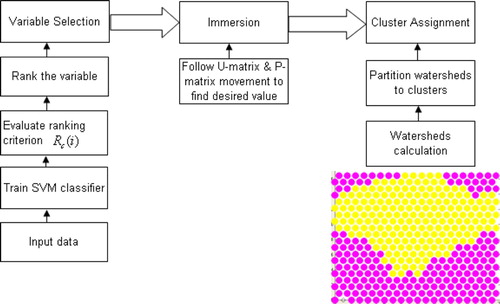
Our proposed methodology to realise the questionnaire approach for emotion profiling is an algorithmic approach which comprises the SVM-based criterion-ranking feature selection and ESOM for unsupervised classification. Figure 1 shows the flow diagram that illustrates the ESOM with support-vector ranking (SVESOM). The SVM is trained using the full set of input data and the ranking criterion is evaluated for feature ranking. The data are then clustered by the ESOM algorithm and such clusters are assigned for classification. The input space consists of the full attributes data. R _c is the ranking criteria and Var provides the vector that ranks the best features in ascending order. The algorithms will be described later in this section.

Figure 1. The flow structure of the emergent self-organising learning with support-vector feature ranking. The SVM is trained using the full set of input data and the ranking criterion is evaluated for feature ranking. The data are then clustered by the ESOM algorithm and such clusters are assigned for classification.

2.1. Support vector ranking

Features are described by the vector that consists of all features used in representing the instance of data. Feature selection is a relatively important step in highly imbalanced situations. Instead of balancing the training data, the first part of this work actively selects the most useful features that alleviate the imbalance effect. The imbalance effect makes the data highly skewed prior to processing (Chawla, Japkowicz, and Kolcz 2003; Chawla, Japkowicz, and Zhou 2009). The support vector ranking is able to find the least skewed feature and hence gives this feature with a high ranking. On the other hand, a feature that made the data distribution skewed is given a low ranking. In this manner, the selected features reduce the imbalance effect in the data. The purpose of selecting the most useful features is to eliminate irrelevant features to enhance the generalisation performance of a given learning algorithm. The selection of relevant features is useful to provide an alternative to handle the imbalanced data problem. Other advantages may include cost reduction of data gathering and storage particularly in this questionnaire data set.

This work employs the use of a derivation of support vector for variable selection. It was initially proposed by Guyon, Weston, Barnhill, and Vapnik (2000) for selecting genes that are relevant for a cancer classification problem. The goal is to find a subset of size r among d features where r<d which maximises the performance of classifiers (Rakotomamonjy 2003). The method is based on backward sequential selection. The features are removed one at a time until r features. The criteria for selection are derived from SVMs and are based on weight vector sensitivity with respect to the feature (Guyon et al. 2000). This is an extension to bounds on L error, margin bound and other bounds of the generalisation error (Rakotomamonjy 2003). The criteria being investigated is C _t which is either weight vector , the radius/margin bound or the span estimate. It gives either an estimation of the generalisation performance or an estimation of the data set separability. The removed variable is the one whose removal minimises the variation of . Hence, the ranking criterion R _c for a given variable i is

where K ⁽ⁱ⁾ is the Gram matrix of the training data when variable i is removed, such that ( and is the solution of quadratic optimisation problem. From the above equation, the removed variable is the one which has the least influence on the weight vector norm.

This approach of criteria-ranking derived from SVM is different from the popularly used soft margin SVM. In traditional SVM where given a set of labelled instances and a kernel function k, SVM finds the optimal α_t for each x _i to maximise the margin γ between the hyperplane and the closest instances to it. The prediction for a new sample x is made through

where b is the threshold, \!\!. One norm soft-margin SVM minimises the primal Lagranian:

where and r _i ≥0. The penalty constant C represents the trade-off between the empirical error ξ and the margin. Two approaches (Rakotomamonjy 2003) are proposed for each criterion:

•	Zero-order method: The criterion C t is directly used for variable ranking, and it identifies the variable that produces the smallest value of C t when removed. The ranking criterion becomes , with C t (i) being the criterion value when variable i has been removed.
•	First-order method: This uses the derivatives of the criterion C t with regard to a variable. This approach differs from the zero-order method because a variable is ranked according to its influence on the criterion which is measured with the absolute value of the derivative.

The algorithms are listed as below:

Algorithm

SVM-based ranking for variable selection

Repeat the following until Var is not empty:

1.	Train an SVM classifier with all the training data and variable Var.
2.	For all Var, evaluate ranking criterion R c (i) of variable i
3.
4.	Rank the variable that minimises R c:
5.	Remove the variable that minimises R c from the selected variables set

2.2. Emergent self-organising map

After finding the top-ranked features, we then use the features for ESOM. The ESOM is a nonlinear projection technique using neurons arranged on a map. It is an extension of self-organising map (SOM) where the neurons go through competitive learning. There are several reasons for using ESOM. Firstly, ESOM allows the discovery of knowledge using its emergent property. This makes it particularly useful for dealing with the problem in this work which consists of several thousands of data. Secondly, the self-adaptive structures are fast and incrementally discover the underlying structure. This allows fast computation even when the data set is large.

The goal of SOM is to transform an incoming signal pattern of arbitrary dimension into a one- or two-dimensional discrete map, and to perform this transformation adaptively in a topologically ordered fashion. Kohonen (1990) describes SOM as a nonlinear, ordered, smooth mapping of high-dimensional input data manifolds onto the elements of a regular, low-dimensional array. Assume the set of input variables {ξ _j } is definable as a real vector . With each element in the SOM array, we associate a parametric real vector that we call a model. Assuming a general distance measure between x and m _i denoted d(x, m _i ), the input vector x on the SOM array is defined as the array element m _c that matches best with x, i.e. that has the index

The task is to define m _i in such a manner that the mapping is ordered and descriptive of the distribution of x. The data points that are projected to close-by locations on the map are also close-by in the input space. The ability of self-organising according to neuron's neighbourhood Euclidean distance is the key feature of SOM. However, the power of self-organising that allows the emergence of structure in data is often neglected (Ultsch and Mörchen 2005). The concept of boundless maps (e.g. Toroids map) to avoid border effect is rarely used. These motivate this particular choice of scaling parameters in the ESOM (Ultsch and Mörchen 2005).

The ESOM is a nonlinear projection technique using neurons arranged on a map. The ESOM forms a low-dimensional grid of high-dimensional prototype vectors. The density of data in the vicinity of the models associated with the map neurons, and the distances between the models, are taken into account for better visualisation. An ESOM map consists of a U-Map (from U-Matrix), a P-Map (from P-Matrix) and a U*-Map (which combines the U and P map). The three maps show the layout for a landscape like visualisation for distance and density structure of the high-dimensional data space. Structures emerge on top of the map by the cooperation of many neurons. These emerging structures are the main concept of ESOM. It can be used to achieve visualisation, clustering and classification. The different maps for visualisation and the clustering algorithm are introduced in the following sections.

2.2.1. Map visualisation

Let m:D→M be a mapping from a high-dimensional data space onto a finite set of positions arranged on a grid. Each position has its two-dimensional coordinates and a weight vector which is the image of a Voronoi region in D: the data set with x _i ∈D is mapped to a position in M such that a data point x _i is mapped to its best-match with , where d is the distance on the data set. The set of immediate neighbours of a position n _i on the grid is denoted by N(i).

2.2.2. U-Map (distance-based visualisation)

The U-height for each neuron n _i is the average distance of n _i ’s weight vectors to the weight vectors of its immediate neighbours N(i). The U-height, denoted uh(i), is calculated as follows:

A display of all U-heights on top of the map is called a U-Matrix (Ultsch and Siemon 1990). The height value will be large in area where no or few data points reside, creating mountain ranges for cluster boundaries. The sum will be small in area of high densities. A U-Map is a height-field like visualisation of the U-Matrix. The local distance structure is displayed at each neuron as a height value creating a three-dimensional landscape of the high-dimensional data space.

2.2.3. P-Map (density-based visualisation)

The P-height ph(i)for a neuron n _i is a measure of the density of data points in the vicinity of w _i :

A display of all P-heights on top of the grid G is called a P-Matrix. The radius r should be chosen such that ph(i) approximates the probability density function of the data points. Distance-based methods usually work well for clearly separated clusters; problems can occur with slowly changing densities and overlapping clusters. Density-based methods directly measure the density in the data space sampled at the prototype vectors. The P-Matrix displays the local density measures with Pareto density estimation (Ultsch 2003).

2.2.4. U*-map (distance and density based visualisation)

For the identification of clusters in data sets, it is sometimes not enough to consider distances between the data points. The local distance depicted in an U-Matrix is presumably the distance measured inside a cluster for the dense region, such distance is often disregarded for clustering purposes. However, in the less-dense region, such a distance is important where the U-Matrix heights correspond to cluster boundaries. This leads to the definition of an U*-Matrix described in Ultsch (2005). The U*-matrix combines the distance-based U-Matrix and the density-based P-Matrix. The U*-matrix shows significant improvement over U-Matrix in data set with clusters that are not clearly separated in the high-dimensional space.

uh(i) is denoted by the U-height of a neuron i, denotes the mean of all P-heights and is the maximum of all P-heights. The U*-height, denoted as u* h(i), of an U-Matrix for neuron i is calculated as

where λ (i) is denoted as a scaling factor which is calculated as

With this equation, the scaling factor basically is a linear function of the P-heights. Using this scaling factor, the U*-height is equalled to U-height if of neuron i. We expect the probability density function of P-height is bimodal and its density distribution is a combination of the within cluster density distribution and the densities of weight vectors in between clusters.

2.2.5. ESOM clustering and classification

After finding the top-ranked variables, we then employ the features for clustering at the ESOM. The ESOM is a nonlinear projection technique which forms a low-dimensional grid of high-dimensional prototype vectors. The density of data in the vicinity of the models associated with the map neurons and the distances between the models are taken into account for better visualisation. Unlike standard Kohonen map (Kohonen 1990) and the other mapping methods like manifold embedding (Roweis and Saul 2000; Rao, Hero, States, and Engel 2006; Nie, Xu, Tsang, and Zhang 2010) which are only a single mapping approach, the ESOM is a multiple mapping approach which consists of three maps, i.e. a U-Map (from U-Matrix), a P-Map (from P-Matrix) and a U*-Map (which combines the U and P map), in which these three maps would show a landscape to visualise the distance and density structure of the high-dimensional data space. Such structures emerge on top of the map by incorporating many neurons. These emerging structures are the main concept of ESOM which can be used to achieve visualisation, clustering and classification. The clustering algorithm is described by the following.

Let m:D→M be a mapping from a high-dimensional data space onto a finite set of positions arranged on a grid. Each position has its two-dimensional coordinates and a weight vector which is the image of a Voronoi region in D: the data set with x _i ∈D is mapped to a position in M such that a data point x _i is mapped to its best match with , where d is the distance on the data set. The set of immediate neighbours of a position n _i on the grid is denoted by N(i).

The clustering of ESOM is based on the U*C clustering algorithm described by (Ultsch 2005). Consider a normalised data point x at the surface of a cluster C, with a best match of n _i =bm(x). The neighbourhood size starts from 25 units and gradually reduced to 1. The weight vectors of its neighbours N(i) are either within the cluster, in a different cluster or interpolate between clusters. Assume that the inter cluster distances are locally larger than the local within-cluster distances, then the U-heights in N(i) will be large in such directions which point away from the cluster C. Thus, a so-called immersive movement will perform to lead away from cluster borders. It is a movement from one position n _i to another position n _j with the result that w _i is more within a cluster C than w _j . This immersive movement is performed which starts from a grid position, keeps decreasing the U-Matrix value by moving to the neighbour with the smallest value, then keeps increasing the P-Matrix value by moving to the neighbour with the largest value.

Finally, the classification phase is performed to determine an emotion category C _j which the test image belongs to, . The clustering process assign input image x to a cluster C _j according to its feature vector. After that, the clusters are pre-labelled with the respective emotion category. The class is determined by taking the cluster whose Euclidean distance is nearest to the test vector.

The details of this clustering algorithm can be referred to Ultsch (2005) and the algorithm is summarised as follows:

Algorithm

ESOM clustering

Initialisation:

1.	Determine the topology and size of network
2.	Initialise the weights of the neurons and initial learning rates
3.	The input vectors are normalised to the range of 0–1.

Immersion:

For each input x, we find the best matched n neuron and construct the matrix as follows:

1.	From position n follow a descending movement on the U-matrix until the lowest distance value is reached in position u.
2.	From position u follow an ascending movement on the P-Matrix until the highest density value is reached in position p.
3.	.

Cluster assignment:

1.	Calculate the watersheds for the U*-matrix using the algorithm in (Luc and Soille 1991).
2.	Partition I using these watersheds into clusters .
3.	Assign a data point x to a cluster C j if Immersion (bm,(x))∈C j .

Classification:

1.	For each test vector; calculate the Euclidean distance from each cluster.
2.	The class of the test vector belongs to the label of the cluster with nearest Euclidean distance to test vector.

3. Experimental results and discussion

The experiments were carried out using three stratified cross-validation training and test sets. Two-third of the data set constitute testing and the remaining one-third is for training. The questionnaire data are arranged into two class problem, for instance, joy classification consists of joy emotion versus non-joy emotion and similarly for the other emotions. The ratios of the emotions are maintained in the cross-validation experiments. The ISEAR data set was constructed by a group of psychologists in 1990 (Geneva Emotion Research Group 1990). Student respondents, both psychologists and non-psychologists, were asked to report situation in which they had experienced the seven major emotions (joy, fear, anger, sadness, disgust, shame, and guilt). In each case, the questions covered the way they had appraised the situation and how they reacted. The ISEAR contains 37 variables as illustrated in Table 2. This section starts with analysing the important features selected and how these features link to psychological states and behaviour. The receiver operating characteristic (ROC) analysis and performance measurements are discussed in Sections 3.2 and 3.3. Lastly, the data visualisations are shown to demonstrate the distribution of data after clustering.

3.1. Feature ranking analysis

The priority of the variables represented by feature ranking corresponding to different emotions is tabulated in Table 3. The corresponding interpretations of variables are shown in Table 2. The ten selected features are meant to describe an emotion collectively. Joy is a happy emotion and it is usual that it lasts long (LONG). When a subject experiences joy, he/she is less likely to control (CON) or hide the emotion as it is felt intensely (INTS). Laughter is the result of expressing (EXP1) joyfulness. Fear is an emotion that is difficult to cope with (COPING) or control as it is an emotion with great obstacles to work with. It takes some time (LONG) for this feeling to subside. Anger is another emotion which is difficult to control (CON) (Wilkowski and Robinson 2008). The subject expresses anger through facial expression directly (EXPRES) or speaking (VERBAL) about the anger felt. The expression of anger differs between individuals. Figure 2 (third picture from left) shows an anger face with lowered eyebrows, straightened lower eyelids and tensed lips. Sadness is a difficult feeling to cope with (COPING) and it persists for a long period of time (LONG). If the sadness continues to linger for a longer period of time, it could lead to depression, which affects subject's relationship with others (RELA). Disgust, shame and guilt are emotions that people find difficult to cope with (COPING) as they belong to the negative emotions which are unpleasant. Disgust typically comes with facial expressions (EXPRES) like wrinkled nose with eyebrows pulled down, upper lip drawn up, lower eyelid is tensed and eye opening narrowed as shown in Figure 2 (second picture from right). Guilt is an intense (INTS) emotion which can be difficult to control (CON) and cope with (COPING). Some people deal with guilt by turning to self-destructive behaviour such as excessive drinking. The ten features selected for each emotion as tabulated in Table 3 collectively explain the emotion and the distinguishing attributes to differentiate the different emotions.

Figure 2. Six basic emotions and neutral expression from JAFEE database (Lyons, Budynek, and Akamatsu 1999).

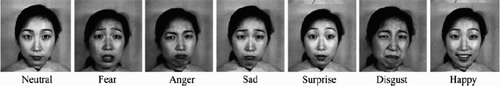
Table 3. Feature ranking by SVESOM for seven different emotions.

Feature ranking	1	2	3	4	5	6	7	8	9	10
Joy	PLEA	LONG	CON	ERGO	TEMPER	PLAN	EXPC	EXP1	MORL	INTS
Fear	COPING	CAUS	INTS	ERGO	FAIR	MORL	EXPRES	VERBAL	LONG	PLAN
Anger	WHEN	CAUS	LONG	VERBAL	PLAN	MOCC	FOCC	EXPRES	CON	ERGO
Sad	RELA	LONG	CAUS	FOCC	COPING	MORL	WHEN	NEUTRO	EXPC	PLAN
Disgust	COPING	PLAN	WHEN	MORL	PLAN	FAIR	EXPRES	ERGO	SEX	PRAC
Shame	COPING	EXPC	PRAC	WHEN	LONG	INTS	PARAL	MORL	CAUS	VERBAL
Guilt	AGE	COPING	FAIR	WHEN	LONG	CON	RELA	INTS	MORL	PLAN

3.2. Sensitivity and specificity

Sensitivity and specificity measures are adopted in our experiments. Basically, sensitivity and specificity are statistical performance measures of a binary classification test. The sensitivity measures the proportion of actual positives which are correctly identified. The specificity measures the proportion of negatives which are correctly identified. The sensitivity and specificity are calculated between the values of true positive (TP), false negative (FN), false positive (FP) and true negative (TN). The formulas of sensitivity and specificity are given by the followings:

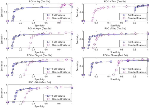
Recall or sensitivity is the percentage of the positive labelled instances which are predicted as positive. Specificity is the percentage of negative labelled instances that are predicted as negative. The sensitivity and specificity are used for plotting the ROC curve to illustrate their performances. The ROC curves of the training and test sets are shown in Figures 2 and 3, respectively. In this ROC analysis, the curve is plotted by the function of sensitivity against specificity for different cut-off points. This demonstrates a trade off between the rates of TP and FP provided with different classification criteria. The perfect classification, i.e. no overlapping in both distributions of sensitivity and specificity, means that the ROC curve would pass through the upper left corner. As shown in Figures 3 and 4, by using both four highest ranking features and full features respectively, good ROC performances can be achieved for all the emotions considered. For consistency, we took four most discriminative features in this ROC analysis for all the seven types of emotions. The four features vary with different profiling of emotions. By taking the joy emotion for example, the four selected features correspond to pleasant, duration, control, and ergotropic. The analysis for the feature ranking will be discussed in the next sub-section.

Figure 3. The ROC analysis with using top four most discriminative features versus full features in training set of questionnaires emotion data.

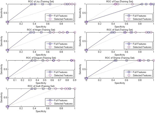
Figure 4. The ROC analysis of using top four most discriminative features versus full features in test set of questionnaires emotion data.

3.3. Performance evaluations

Accuracy may not be an appropriate measure to evaluate the performance of classifiers for this emotion data set. A classifier may be able to obtain a very high accuracy by classifying all instances to majority class but classifying wrongly the minority class. Therefore, the use of accuracy and mean square error rate are inappropriate for IDS like this emotion data set. So we adopted the use of other kinds of evaluation metrics to measure the classifiers’ capability to differentiate the two-class problem under the case of imbalanced data distribution. They are namely, F-measure and geometric means measure (GMM), in which the performance measures are independent of prior probabilities. F-measure is a metric derived from recall and precision. Some variants would make the weighting equal as it is considered that the occurrences of FP and FN are likely equal. According to the evaluations by Barandela, Sánchez, García, and Rangel (2003), GMM is a more appropriate metric to evaluate the classifier performance on the data sets which are imbalanced distribution. Both F-measure and GMM are good indicators as they maximise the accuracy on each of the two classes while keeping these accuracies balanced. The GMM is defined as the square root of the product of accuracy on positive samples and negative samples (i.e. and . Their formulas are shown below:

where

where

The experimental results are shown in Tables 4–6. Three sets of results are displayed to show the best, moderate and the worst performances among the seven emotions of joy, fear, anger, sadness, disgust, and guilt. In these tables, each row represents different numbers of selected features as the input to perform the classifiers. The corresponding results in terms of generalisation, sensitivity, F-measure, geometric means’ measure for both training and test data sets are shown in each column of the tables. Joy is the most easily distinguished emotion, with F-measure constantly above 90%. The first three features are insufficient to allow the competitive learning of ESOM to converge. However, with the use of four features onwards, the convergence ensures. It demonstrates that the use of more features or full features does not guarantee a higher performance in terms of F-measure, generalisation and geometric means. The result is consistent with the other emotions like anger, shame and etc. Most of the experiments in different emotional profiling are converged if more than three features were used. The fear emotion in Table 5 shows the median results among the emotions; the average results of the common emotions are around 72%. It is also noted that there is no significant improvement by increasing the number of features more than four. It can be concluded that using four features are sufficient to profile the emotion by this questionnaire data set in most cases. Moreover, the results of F-measure, which is the main performance metrics for imbalance data sets, often maintain at a relative high level of 0.7 or above. Note that disgust is a difficult emotion to be classified because the data collected from questionnaires do not have significant variations between the variables (Scherer 1997).

Table 4. Performance result of joy emotion by SVESOM.

Features	Generalisation	Sensitivity	F-measure	GMts	GMtr
2	Cannot converge
3
4	0.96	0.97	0.96	0.94	0.98
5	0.96	1.00	0.98	0.91	1.00
6	0.94	0.99	0.96	0.87	0.99
7	0.95	0.99	0.97	0.87	0.99
8	0.96	0.99	0.98	0.93	1.00
All	0.95	1.00	0.97	0.91	1.00

Table 5. Performance result of fear emotion by SVESOM.

Features	Generalisation	Sensitivity	F-measure	GMts	GMtr
2	Cannot converge
3	0.65	0.75	0.70	0.54	0.84
4	0.63	0.80	0.70	0.44	0.88
5	0.65	0.86	0.74	0.47	0.91
6	0.70	0.84	0.77	0.49	0.90
7	0.67	0.86	0.75	0.36	0.91
8	0.63	0.84	0.72	0.45	0.90
All	0.81	0.96	0.88	0.53	0.84

Table 6. Performance result of disgust emotion by SVESOM.

Features	Generalisation	Sensitivity	F-measure	GMts	GMtr
2	Cannot converge
3	0.60	0.74	0.66	0.54	0.84
4	0.71	0.89	0.79	0.52	0.93
5	0.73	0.90	0.81	0.53	0.94
6	0.70	0.90	0.79	0.47	0.94
7	0.77	0.90	0.83	0.56	0.94
8	0.72	0.93	0.82	0.43	0.96
All	0.85	0.87	0.86	0	0.35

In addition, the result obtained by our approach was benchmarked with the work of Danisman and Alpkocak (2008) in which the so-called vector space model (VSM) was adopted to classify the ISEAR data set and achieve an overall F-measure of 0.68 for five types of emotions (see the results detail in Danisman and Alpkocak (2008)). The overall benchmarking results are tabulated in Table 7. The results show that our SVESOM model outperforms the VSM model since all the seven types of emotions were analysed in this ISEAR data set and an overall F-measure of 0.82 was achieved by our proposed model. Moreover, our analysis gave individual results of the different emotions as opposed to the Danisman and Alpkocak approach, which only showed the overall classification result for this ISEAR data set.

Table 7. ISEAR benchmarking results between Danisman and Alpkocak (2008) versus our approach.

Measure	SVM five class emotions (Danisman and Alpkocak 2008)	SVESOM seven class emotions
Kappa^a	0.59	0.68
F-measure	0.675	0.82
Accuracy	0.674	0.8
^aKappa measure is a metric to measure the degree of agreement or disagreement of two or more people observing the same phenomenon. It can be implemented into any classifier that it is preferable to just counting the number of misses – even for those cases where all errors can rightfully be treated as being of similar importance (Arie 2008).

3.4. Data visualisation

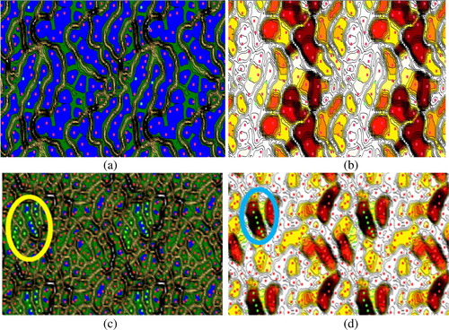
This section presents the data visualisation results generated by the ESOM with selected features as shown in Figure 5. ESOM maps the original data features onto two-dimensional axis. The locations of the datapoints represent the trained neurons after the competitive learning. The U-Matrix realises the distances of the emergence of structural features within the data space. Two-dimensional toroid structure with Euclidean distance was adopted for the ESOM mapping. The adjacent U-matrix can be combined together to form a ‘boundless’ picture for such data distribution, for example the majority of the samples in red (Figure 5(c) and (d)) are distributed around the edges of the map. The structure of high-dimensional data would be extracted from major blocks of the visualised results in the centre of U-Map. The questionnaire data set can be visualised in the map space. The cluster of the minority class (i.e. the green points) is formed amidst the majority class (i.e. the red points). The maps show the visualisation of the shame emotion denoted as green points, whereas red points denote non-shame emotion. The darker colour of the background in U-Map implies larger separation between the neighbouring data points. Similarly, darker background colour in the P-Map implies that the area is denser. As shown in the maps of Figure 5(c) and (d), with the use of four features selected, the clusters of minority class started appear as circled in the figures, The map is a tiled display of multiple maps and hence the cluster is repeated in the other regions. This is in contrast with Figure 5(a) and (b) which used only two features; the maps are not able to converge with defined clusters. The ESOM provides a low-dimensional projection preserving the topology of the input space, thus the high-dimensional distances can be visualised with the canonical U-Matrix, P-Matrix and U*-Matrix together so that the cluster boundaries can be distinguished more sharpely. In addition, the visualisation by the ESOM feature map can be interpreted as height values on top of the usually two-dimensional grid of the SOM, leading to an intuitive paradigm of a landscape. In summary, the visualisation results obtained by the ESOM can help in recognising and classifying consistent emotions in IDS.

Figure 5. Visualisation of questionnaire emotion data (shame) generated by SVESOM under different numbers of features selected. (a) U-map with two features selected; (b) P-Map with two features selected; (c) U-Map with four features selected; (d) P-Map with four features selected; red points denote data points from majority class, whereas green points represent samples from minority class.

4. Conclusion

This study discusses the use of a computational analysis of the questionnaires to understand emotions. The questionnaires method approaches the subject by investigating the real experience accompanying the emotions, whereas the other laboratory approaches are generally embedded with exaggerated elements by asking the subjects to make artificial and exaggerated facial expressions. A connectionist model called the SVESOM was proposed to analyse this questionnaires method. The SVESOM first identifies the significant variables with high ranking and selects them as the dominant features. Those dominant features are in line with the work by Scherer's group, which approaches the emotions physiologically. Then, a self-organising mapping was used to cluster the selected features for classification. The performance measurements showed that it is not necessary to use the full features for classifications, but using the selected features is sufficient to provide superior results in terms of accuracy and generalisation. The further study is gearing towards the profiling of deeper emotion understanding that maps the emotion to infer how humans think, desire or believe to be the driving factors behind human expressions. This work will provide the capability to infer mental states of people from their facial expressions. This study acts as the foundation which establishes an expert variables’ interpreter that ultimately leads to better classification decisions.

References

- Arie , B.-D. 2008 . Comparison of Classification Accuracy using Cohen's Weighted Kappa . Expert Systems with Applications , 34 ( 2 ) : 825 – 832 .
- Ball , G. and Breese , J. 2000 . “ Emotion and Personality in a Conversational Agent ” . In Embodied Conversational Characters , Edited by: Prevost , S. , Cassell , J. , Sullivan , J. and Churchill , E. Cambridge , MA : MIT Press .
- Barandela , R. , Sánchez , J. S. , García , V. and Rangel , E. 2003 . Strategies for Learning in Class Imbalance Problems . Pattern Recognition , 36 ( 3 ) : 849 – 851 .
- Chawla , N. V. , Japkowicz , N. and Kolcz , E. A. Special Issue on Learning from Imbalanced Data Sets . Proceedings of the ICML’2003 Workshop on Learning from Imbalanced Data Sets .
- Chawla , N. , Japkowicz , N. and Zhou , Z. H. Data Mining When Classes are Imbalanced and Errors Have Costs . PAKDD’2009 Workshop . Thailand
- Danisman , T. and Alpkocak , A. 2008 . “ Feeler: Emotion Classification of Text Using Vector Space Model ” . In AISB Communication, Interaction and Social Intelligence
- Darwin , C. 1872 . The Expression of the Emotions in Man and Animals , London : John Murray Press .
- Davidson , R. J. , Schwartz , G. E. , Saron , C. , Bennett , J. and Goleman , D. 1979 . Frontal Versus Arietal EEG Asymmetry during Positive and Negative Affect . Psychophysiology , 16 : 202 – 203 .
- Desseilles , M. J. , Schwartz , S. , Dang-Vu , T. T. , Sterpenich , V. , Darsaud , A. , Albouy , G. , Gais , S. , Schabus , M. and Rauchs , G. 2006 . Effects of Attention and Emotion on Face Processing in Depression: A Functional MRI Study . European Neuropsychopharmacology , 16 ( Supplement 4), S271–S271 )
- Ekman , P. 2004 . Emotions Revealed , New York : Henry Holt and Company LLC . First Owl Books
- Ekman , P. and Friesen , W. V. 1971 . Constants Across Cultures in the Face and Emotion . Journal of Personality and Social Psychology , 17 ( 2 ) : 124 – 129 .
- Geneva Emotion Research Group . 1990 . “ International Survey on Emotion Antecedents and Reactions (ISEAR) ” . http://www.unige.ch/fapse/emotion/databanks/isear.html
- Guyon , I. , Weston , J. , Barnhill , S. and Vapnik , V. 2000 . Gene Selection for Cancer Classification Using Support Vector Machines . Machine Learning , 46 ( 1–3 ) : 389 – 422 .
- Kohonen , T. 1990 . Self-organizing Map . Proceedings of the IEEE , 78 ( 9 ) : 1464 – 1480 .
- Levine , D. 2007 . “ How Does the Brain Create, Change, and Selectively Override its Rules of Conduct? ” . In Neurodynamics of Cognition and Consciousness , Edited by: Perlovsky , L. and Kozma , R. 163 – 184 . Berlin : Springer-Verlag .
- Luc , V. and Soille , P. 1991 . Watersheds in Digital Space: An Efficient Algorithm Based on Immersion Simulations . IEEE Transactions on Pattern Analysis and Machine Intelligence , 13 ( 6 ) : 583 – 598 .
- Lutfi , S. L. , Montero , J. M. , Barra-Chicote , R. , Lucas-Cuesta , J. M. and Ascensión , G.-A. 2009 . Expressive Speech Identifications based on Hidden Markov Model . HEALTHINF , 2009 : 488 – 494 .
- Lyons , M. J. , Budynek , J. and Akamatsu , S. 1999 . Automatic Classification of Single Facial Images . IEEE Transactions on Pattern Analysis and Machine Intelligence , 21 ( 12 ) : 1357 – 1362 .
- Nie , F. , Xu , D. , Tsang , I. and Zhang , C. 2010 . Flexible Manifold Embedding: A Framework for Semi-supervised and Unsupervised Dimension . IEEE Transactions on Image Processing , 19 ( 7 ) : 1921 – 1932 .
- Nguwi , Y.-Y. and Cho , S.-Y. Support Vector Self-Organizing Learning for Imbalanced Medical Data . International Joint Conference of Neural Networks , pp. 2250 – 2255 . Atlanta , GA
- Perlovsky , L. 2007 . “ Neural Dynamic Logic of Consciousness: The Knowledge Instinct ” . In Neurodynamics of Cognition and Consciousness , Edited by: Perlovsky , L. and Kozma , R. 73 – 108 . Berlin : Springer-Verlag .
- Phan , K. L. , Wager , T. and Taylor , S. F. Functional neuroanatomy of emotion: a meta-analysis of emotion activation studies in PET and FMRI . NeuroImage , 16 331 – 338 .
- Picard , R. 1997 . Affective Computing , Cambridge , MA : The MIT Press .
- Rakotomamonjy , A. 2003 . Variable Selection using SVM Based Criteria . The Journal of Machine Learning Research , 3 : 1357 – 1370 .
- Rao , A. , Hero , A. O. , States , D. J. and Engel , J. D. Manifold Embedding for Understanding Mechanisms of Transcriptional Regulation . Paper presented at the IEEE International Workshop on Genomic Signal Processing and Statistics, 2006 . GENSIPS ‘06
- Redcay , E. , Dodell-Feder , D. , Pearrow , M. J. , Mavros , P. L. , Kleiner , M. , Gabrieli , J. D.E. and Saxe , R. 2010 . Live face-to-face Interaction during fMRI: A New Tool for Social Cognitive Neuroscience . NeuroImage , 50 ( 4 ) : 1639 – 1647 .
- Roweis , S. T. and Saul , L. K. 2000 . Nonlinear Dimensionality Reduction of Locally Linear Embedding . Science , 290 : 2323 – 2326 .
- Scherer , K. R. 1997 . Profiles of Emotion-antecedent Appraisal: Testing Theoretical Predictions Across Cultures . Cognition and Emotion , 11 : 113 – 150 .
- Scherer , K. R. 1997 . The Role of Culture in Emotion-antecedent Appraisal . Journal of Personality and Social Psychology , 73 : 902 – 922 .
- Scherer , K. R. and Wallbott , H. G. 1994 . Evidence for Universality and Cultural Variation of Differential Emotion Response Patterning . Journal of Personality and Social Psychology , 66 : 310 – 328 .
- Sears , A. and Jacko , J. A. 2008 . The Human-Computer Interaction Handbook: Fundamentals, Evolving Technologies, and Emerging Applications , 2 , USA : CRC Press .
- Thorburn , W. M. 1915 . Occam's Razor . Mind , 24 : 287 – 288 .
- Ultsch , A. Pareto Density Estimation: A Density Estimation for Knowledge Discovery . Innovations in Classification, Data Science, and Information Systems – Proceedings 27th Annual Conference of the German Classification Society (GfKL) 2003 . Edited by: Baier , D. and Wernecke , K. D. pp. 91 – 100 . Berlin, Heidelberg : Springer .
- Ultsch , A. 2005 . Clustering with SOM: U*C 75 – 82 . Paris WSOM 2005
- Ultsch , A. and Siemon , H. Kohonen's Self Organizing Maps for Exploratory Data Analysis . Proceedings of International Neural Network Conference (INNC’90 , pp. 305 – 308 .
- Ultsch , A. and Mörchen , F. 2005 . “ ESOM-Maps: Tools for Clustering, Visualization, and Classification with Emergent SOM ” . Germany : Dept. of Mathematics and Computer Science, University of Marburg . Technical Report No. 46
- Ververidis , D. and Kotropoulos , C. 2006 . Emotional Speech Recognition: Resources, Features, and Methods . Speech Communication , 48 ( 9 ) : 1162 – 1181 .
- Wallbott , H. G. and Scherer , K. R. 1985 . “ Analysis of Nonverbal Behaviour ” . In Handbook of Discourse Analysis 2 , Edited by: Van Dijk , T. A. 199 – 230 . USA : Blackwell .
- Wallbott , H. G. and Scherer , K. R. 1988 . Emotion and Economic Development – Data and Speculations Concerning the Relationships Between Economic Factors and Emotional Experience . European Journal of Social Psychology , 18 : 267 – 273 .
- Westen , D. , Blagov , P. S. , Harenski , K. , Kilts , C. and Hamann , S. 2006 . Neural Bases of Motivated Reasoning: An fMRI Study of Emotional Constraints on Partisan Political Judgment in the 2004 U.S. Presidential Election . Journal of Cognitive Neuroscience , 18 ( 11 ) : 1947 – 1958 .
- Wilkowski , B. M. and Robinson , M. D. 2008 . Guarding Against Hostile Thoughts: Trait Anger and the Recruitment of Cognitive Control . Emotion , 8 ( 4 ) : 578 – 583 .