Robust manifold learning with CycleCut

Abstract

Many manifold learning algorithms utilise graphs of local neighbourhoods to estimate manifold topology. When neighbourhood connections short-circuit between geodesically distant regions of the manifold, poor results are obtained due to the compromises that the manifold learner must make to satisfy the erroneous criteria. Also, existing manifold learning algorithms have difficulty in unfolding manifolds with toroidal intrinsic variables without introducing significant distortions to local neighbourhoods. An algorithm called CycleCut is presented, which prepares data for manifold learning by removing short-circuit connections and by severing toroidal connections in a manifold.

Keywords:

• neighbourhood graphs
• shortcut connection detection
• nonlinear dimensionality reduction
• manifold learning

1. Introduction

In the last decade, manifold learning has become a significant component of machine learning, data mining, vision, and robotics. In machine learning and data mining, manifold learning can be used to reduce dimensionality, which otherwise presents a significant challenge for many algorithms. In vision and robotics, manifold learning is used to reduce a sequence of images to a corresponding sequence of ‘intrinsic variables’, which can be used to estimate the state from which the images were obtained.

Many manifold learning algorithms, including locally linear embedding (LLE), Laplacian eigenmap, Hessian LLE, local tangent space alignment, maximum variance unfolding, manifold sculpting, and others, rely on graphs of local neighbourhoods to estimate manifold topology. These algorithms seek to ‘unfold’ a collection of samples from the manifold to occupy fewer dimensions while preserving distances (or other relationships) between points in local neighbourhoods. The quality of the results obtained from these algorithms is limited by the quality of the neighbourhood graphs. If the local neighbourhoods contain connections that short-circuit across manifold boundaries, the manifold learner will seek a compromise embedding that satisfies each neighbourhood relationship to varying degrees, including the short-circuit connection. Such compromise solutions constitute poor results.

We present an algorithm called CycleCut, which identifies and ‘cuts’ the neighbourhood connections that short-circuit across the manifold. In contrast with the existing algorithms, CycleCut efficiently finds a minimal set of connections for removal such that there are no topological holes represented in the manifold. It guarantees not to segment the graph, and under common conditions (which we define in Section 3.1), it also guarantees to remove all short-circuiting connections. Even when these conditions do not hold, it tends to exhibit a desirable behaviour for improving the results of manifold learning. This paper is laid out as follows: Section 2 reviews related work. Section 3 presents the CycleCut algorithm. Section 4 gives an analysis of this algorithm, including a complexity analysis and empirical results. Section 5 concludes by discussing future work.

2. Related work

It has long been known that manifold learning algorithms have difficulty when local neighbourhood connections short-circuit (or shortcut) across the manifold (Balasubramanian and Schwartz 2002; Varini, Degenhard, and Nattkemper 2006). A simple solution is to use smaller local neighbourhoods, but this risks breaking connectivity and often reduces the quality of results from manifold learning.

A better approach to mitigate this problem involves adaptively selecting local neighbourhoods (Wei, Peng, Lin, Huang, and Wang 2008). This can make the neighbourhood graphs more robust to difficult topologies, but it cannot handle the case where the closest neighbour of a point cuts across the manifold. An approach called manifold denoising (Hein and Maier 2006) has been used to reduce noise in the data and thus decrease the risk of shortcut connections. This technique, however, does directly seek to remove shortcut connections and does not provide any guarantees.

Perhaps the most effective method currently used for identifying shortcut connections is based on edge betweenness centrality (EBC) (Brandes 2001). EBC is a metric that counts the number of times the pair-wise shortest paths between every pair of points pass over each edge. Because shortcut connections join geodesically distant regions of the manifold (by definition), they tend to have higher EBC values than other edges (Cukierski and Foran 2008). The drawbacks of this approach are that it sometimes removes edges that are not shortcuts, and it provides no inherent stopping criteria, requiring that heuristics be used to decide when shortcut edges have been removed. By contrast, we show that graphs with shortcut connections necessarily contain large cycles, and CycleCut guarantees to remove a minimal set of edges to remove all large cycles in the graph.

3. CycleCut

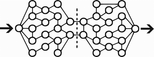
The CycleCut algorithm is inspired by max-flow/min-cut methods for graph partitioning. These methods identify the minimal cut to partition a graph by simulating flow across the graph in order to identify the minimal set of edges that limit the flow as illustrated in Figure 1. The max-flow/min-cut theorem ensures that a cut which removes only the limiting edges is optimal with respect to minimising the sum capacity of the cut edges (Ford and Fulkerson 1962).

Figure 1. Max-flow/min-cut methods simulating flow across a graph to identify a minimal set of edges that limit the flow.

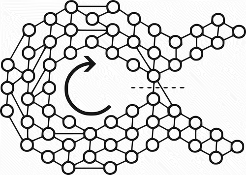
Instead of simulating flow across a graph, CycleCut simulates flow around a topological hole in order to find a minimal cut that breaks the cycles that enclose the hole, as illustrated in Figure 2.

Figure 2. CycleCut simulating flow around a topological hole to identify a minimal set of edges that limit the flow.

There are three common cases when topological holes occur in sampled manifolds: shortcut edges, toroidal intrinsic variables, and unsampled regions. These cases are illustrated in Figure 3. We will describe these cases using an example of a robot which uses a camera to explore a park. The images that this robot obtains with its camera may be considered to be samples on a manifold. If these samples are ‘well-behaved’, manifold learning can be used to obtain a sequence of intrinsic variables that correspond with the sequence of images. These intrinsic variables will include a representation of the robot's estimated position within the park, which would be useful information for many tasks.

Figure 3. Case 1: For manifolds with a topological hole due to shortcut edges, CycleCut reduces distortion in the results. Case 2: For manifolds with topological holes due to toroidal intrinsic variables, CycleCut reduces distortion at the cost of continuity in the results. Case 3: For manifolds with topological holes due to unsampled regions, CycleCut has little effect on the results.

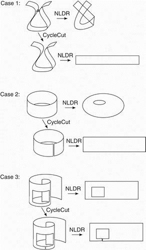
Case 1: Suppose that there are two benches in this park with a similar appearance. Images of these benches would constitute samples on the manifold with a large geodesic distance, but a small observed distance. Thus, the neighbourhood graph of these samples will contain shortcut connections between these observations. These shortcut connections create a topological hole in the sampled manifold. CycleCut will remove the minimal set of edges, such that the topological hole is eliminated. This enables the manifold to be learned without trying to preserve superfluous distances between points.

Case 2: Suppose that the robot has the ability to rotate yaw-wise. Because rotation inherently repeats, the manifold sampled by the robot's images will connect to itself to form an open-cylinder topology. Such manifolds cannot be projected into their tangent-space dimensionality without either introducing distortions or breaking continuity. If the cylinder is tall, then using distortion is a particularly poor solution. CycleCut finds a minimal break in continuity to enable the manifold to be unfolded with little distortion. When CycleCut is not used, resulting points are crowded together near the inner circumference and stretched apart near the outer circumference. Distortion-free estimates of a state space are particularly important for planning purposes because the effectiveness of generalisation is limited by the consistency within the representation of state.

Case 3: Suppose that there is a large pond in the park into which the robot wisely does not advance. This creates an unsampled region which appears to be a topological hole in the manifold, even though the true manifold is continuous. In this case, it would be better not to use CycleCut prior to manifold learning because it is desirable to preserve the unsampled hole as an artefact in the results. If CycleCut is used in this case, it will cut along the shortest path that connects the unsampled region with the outside area. This cut is superfluous, but it will leave a larger amount of edges intact to define the manifold structure. The impact that such a superfluous cut will have on results depends on how much ‘load’ or ‘tension’ is represented in the cut edges. Fortunately, unlike case 2, case 3 typically involves edges that carry little such tension, so results are generally degraded very little. Thus, if case 1 or 2 is known to also exist in a sampled manifold, or if the nature of a collection of samples is unknown, we recommend using CycleCut prior to manifold learning because the potential cost is low, while the potential benefit is high.

If there are no large sample holes, CycleCut has no effect on results.

3.1. The CycleCut algorithm

In graph theory, a chord is an edge that connects two non-adjacent vertices in a cycle. Cycles with no chords are called induced cycles, chordless cycles, or holes. We generalise the notion of a chord by defining an n-chord to be a path of length n which connects two vertices in a cycle, where n is less than the length of the shortest path on the cycle between the vertices. We refer to a cycle with no n-chords as an atomic cycle. For example, the graph shown in Figure 4 contains three chordless cycles, but only two of them are atomic cycles.

Figure 4. The graph containing three cycles. All three of them are chordless, but only two of them are atomic.

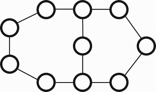
The problem of finding large holes in a graph (as defined by a large chordless cycle) has been well studied (Spinrad 1991; Nikolopoulos and Palios 2004). For the application of preprocessing high-dimensional data for manifold learning, however, large atomic cycles are better indicators of topological holes than large chordless cycles. In a high-dimensional space, irregularly distributed samples frequently create sub-structures like the one shown in Figure 4. If only 1-chords are considered, then large cycles with n-chords (n>1) will be falsely interpreted to indicate that there is a topological hole in the graph, resulting in unnecessary cuts.

The pseudo-code for the CycleCut algorithm is shown in Figure 5. This algorithm can be briefly summarised as follows:

	(1) Equip each edge with a capacity value.
	(2) Find a large atomic cycle, C, else go to Step 7.
	(3) Find the smallest capacity, h, of any edge in C.
	(4) Reduce the capacity of every edge in C by h.
	(5) Remove all edges with a capacity of zero.
	(6) Go to Step 2.
	(7) Restore all removed edges that do not create a large atomic cycle when restored.

Figure 5. Pseudo-code for the CycleCut algorithm. V is a set of vertices. E is a set of edges. (For convenience, an implementation of CycleCut is included in the Waffles (Gashler 2011) machine learning toolkit, and a switch to invoke it has been integrated with each manifold learning algorithm in that toolkit.)

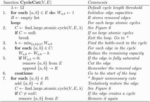
The first step of CycleCut equips each edge with a ‘capacity’ value that indicates the a priori confidence that it represents a good neighbour connection. In this paper, uniform capacities are used, but non-uniform capacities may be used if additional information is available. The second step finds a large atomic cycle in the graph. (We note that this step could be modified, such that any other undesirable structure would be identified and removed from the graph, but in this paper, we are only interested in removing large atomic cycles.) Section 3.2 gives a detailed description of how large atomic cycles are identified. Step 3 finds the minimum capacity, h, of any edge in the large atomic cycle. Step 4 simulates flow by reducing the remaining capacity of every edge in the large atomic cycle by h. Step 5 removes all edges that have become fully saturated. These edges are stored in a list, R. Steps 2–5 are repeated until there are no more large atomic cycles in the graph. Finally, Step 7 restores any edges that were unnecessarily removed in Step 5. Each edge in R is tentatively restored to the graph. If restoring the edge creates a large atomic cycle, then it is removed again. The resulting cut is guaranteed to be minimal with respect to the sum of capacity values, such that all atomic cycles with a cycle length ≥λ are broken.

3.2. The find_large_atomic_cycle routine

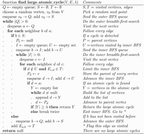
Large atomic cycles are found by iterating over all the atomic cycles in the graph and returning when one with a cycle length ≥λ is found. The pseudo-code for this routine is shown in Figure 6. The atomic cycles in a graph are enumerated using a breadth-first-search (BFS) nested within another BFS. We refer to these as ‘the outer BFS’ and ‘the inner BFS’. The purpose of the outer BFS is to define a region in which the inner BFS is constrained during its search. Whenever the outer BFS detects a cycle (by finding an edge that connects to a vertex that it has already discovered), the inner BFS begins searching from that point. The inner BFS is only allowed to follow edges that the outer BFS has already followed (not including the edge that detected the cycle). The inner BFS terminates when it finds a cycle because subsequent cycles that it would discover would either be the same size or non-atomic.

Figure 6. Pseudo-code to find an atomic cycle with a cycle length≥λ edges in a graph comprising vertices V and undirected edges E.

3.2.1. Proof of correctness

We now give a proof that this routine will find an atomic cycle with a cycle length ≥λ, if some atomic cycle C, , is reachable from the seed point. Let e be the last edge in C to be traversed by the outer BFS, and let T be the set of edges that had been traversed by the outer BFS just before e was traversed. When the outer BFS traverses e, the destination vertex of e is discovered for at least the second time. This event triggers the inner BFS to find a shortest path, P, from one vertex of e to the other, following only edges in T. Let . B must not have any n-chords or else the inner BFS would have arrived at the vertex earlier by cutting across the n-chord. If |B|=|C|, then B satisfies the proof, whether or not B≡ C, and the routine returns. To complete the proof, we show that ‘|B|≠|C|’ is an impossible condition. If |B|>|C|, then the inner BFS would have found C first, so B≡ C, which is a contradiction. If |B|<|C|, then let , where ‘\’ denotes exclusion. A must have been discovered previously or else e would not close both B and C. Furthermore, A must be an atomic cycle or else either B or C would have already been closed. If |A|≥|C|, then , so the routine would have returned when it found A. If |A|<|C|, then A∩B is an n-chord of C, which contradicts the assumption that C is atomic.

4. Analysis and validation

In this section, we analyse the CycleCut algorithm. In Section 4.1, we demonstrate that it is easy to find a good value for λ. In Section 4.2, we give a complexity analysis of CycleCut. In Section 4.3, we demonstrate the use of CycleCut to remove shortcut connections. In Section 4.4, we demonstrate the use of CycleCut to unfold a manifold with a torroidal intrinsic variable.

4.1. The λ threshold

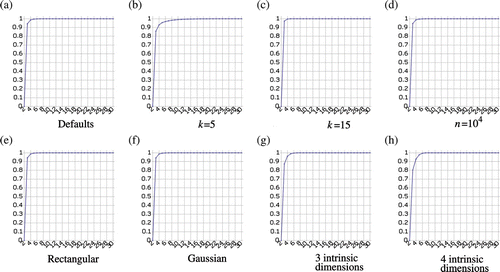
Shortcut edges will always create a large atomic cycle because, by definition, they connect geodesically distant regions of the manifold. As demonstrated in Figure 3 (case 3), it is typically not a problem if a few good connections are cut, but it can cause significant problems if bad connections are not cut. Thus, a good value for λ need only be smaller than the cycles caused by shortcut edges. To show that CycleCut is very robust to the value of λ, we sampled a square region of 2D space with 10⁶ uniformly distributed random points and connected each point with its 10-nearest neighbours. (Many manifolds can be viewed as an embedding of this or a similar structure in a high-dimensional space.) We measured the distribution of the cycle lengths of the atomic cycles in this structure. Figure 7(a) shows the cumulative distribution, with atomic cycle lengths along the horizontal axis and the portion of atomic cycles along the vertical axis. We repeated this experiment with a variety of conditions. In Figure 7(b), 5 neighbours were used instead of 10. In Figure 7(c), 15 neighbours were used. In Figure 7(d), the region was sampled with 100 times fewer points. In Figure 7(e), the sampled region was much wider than tall. In Figure 7(f), samples were drawn from a Gaussian distribution, instead of from a uniform distribution. In Figure 7(g), samples were drawn in three intrinsic dimensions. In Figure 7(h), samples were drawn in four intrinsic dimensions. In every case, the cumulative distribution was approximately the same. This shows that the threshold value λ is robust across a large variety of conditions. As can be seen in each of the charts in Figure 7, the value λ=12 is sufficiently large to handle almost all cases. Thus, we used this value in all our experiments, and it consistently produced good results. In most cases, smaller values, such as λ=8, produced results that were identical to those obtained using λ=12.

Figure 7. The cumulative distribution of the cycle lengths of the atomic cycles from various random distributions of points. In every case, the threshold λ=12 includes nearly all the atomic cycles.

4.2. Complexity

The find_large_atomic_cycle subroutine contains an inner BFS nested within an outer BFS. The outer BFS will visit every edge in the graph. The inner BFS will terminate before following a constant number, k ^λ, of edges, except for the last time it is called, which will terminate before following |E| edges, where E is the set of edges. Thus, the asymptotic computational complexity of find_large_atomic_cycle is O(|E|). The number of times that this subroutine must be called depends on the number of shortcut connections in the graph, so the complexity of CycleCut is bounded between O(|E|) and O(|E|²). If there are few or no shortcuts, CycleCut scales linearly, so it is well suited to be used as a ‘safety-net’ prior to manifold learning. If there are no shortcut connections, as is typically assumed, then little cost is incurred for performing the check, and if there are some shortcut connections, CycleCut can guarantee to catch them.

4.3. Removing shortcuts

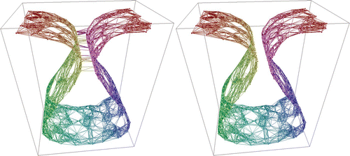
We sampled the manifold with 1000 random values for α and β, where and . Each point was connected with its 14-nearest Euclidean-distance neighbours. Sixty-three of these connections shortcut to geodesically distant regions of the manifold, as shown in Figure 8, left. These shortcut connections would significantly affect the results of most manifold learning algorithms in a negative manner. CycleCut correctly detected and removed all 63 shortcut connections (Figure 8, right). No other connections were cut. (This is an example of case 1 shown in Figure 3.)

Figure 8. Left: One thousand points that are connected with each of their 14-nearest neighbours. Sixty-three of the connections shortcut to geodesically distant regions of the manifold. Right: Removal of all these shortcut connections without removing any other connections by CycleCut.

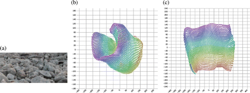
In another experiment, we sampled a manifold by uniformly drawing 50×50 pixel sub-images from a larger image of rocky terrain (Figure 9(a)). Because a certain region on one side of this image was made visually similar to a certain region on the other side, this manifold approaches very close to itself. Figure 9(b) shows results obtained using Isomap with 12 neighbours to reduce 4680 sample sub-images into two dimensions. These values are a poor estimate of the window position. In many cases, it ambiguously assigns similar window positions for very different sub-images. Much better results were obtained using the same algorithm and parameters when the neighbourhood graph was preprocessed with CycleCut (Figure 9(c)). CycleCut removed the connection between some of the images, even though they were very similar, because they created an atomic cycle in the graph. The results obtained with CycleCut are a better estimate of the window position and are sufficiently unambiguous that a model could easily be trained using the resulting data to map from the window position to the sub-image or from the sub-image to the window position.

Figure 9. (a) An image of rocky terrain. We uniformly took 4680 samples from the manifold of 50×50 pixel sub-images with three colour channels of this terrain. Because a certain region on one side of this image is visually similar to a certain region on the other side, this manifold approaches very close to itself. (b) Results obtained using the Isomap nonlinear dimensionality reduction (NLDR) algorithm with 12 neighbours to reduce these 4680 samples into two dimensions. These values are a poor estimate of the window position. In many cases, it ambiguously predicts similar window positions for very different sub-images. (c) Results obtained using the same algorithm and the same number of neighbours, but also using CycleCut to preprocess the neighbourhood graph. These results are a better estimate of the window position and are sufficiently unambiguous that a model could easily be trained using these data to map from the window position to the image or from the image to the window position.

4.4. Toroidal manifolds

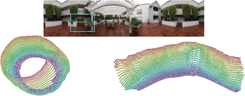
We sampled a panoramic image of a courtyard using a 40×30 pixel sliding window with three colour channels at 225×31 unique window positions (Figure 10). We then used Isomap with 12 neighbours to reduce these data from 3600 to 2 dimensions, both with and without CycleCut. (This is an example of case 2 shown in Figure 3.) In the case where CycleCut was not used, Isomap returned results that ambiguously represented multiple window positions in several regions of the reduced space. When CycleCut was used, it returned results that approximately corresponded to the yaw and pitch represented by the sliding window.

Figure 10. Top: A 40×30 pixel window that was sampled with three colour channels at 225×31 window positions within a panoramic image of a courtyard. (Image derived from a photo by Rich Niewiroski Jr. from the Wikimedia Commons.) Left: A projection of these data by Isomap (Tenenbaum, de Silva, and Langford 2000) with 12 neighbours into two dimensions. Each point is coloured according to the vertical position of the window. Right: A projection by the same algorithm after CycleCut was applied to the neighbourhood map. These values are more meaningful with respect to the yaw and pitch represented by the window.

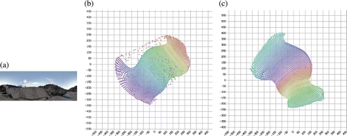
We repeated this experiment using a different panoramic base image. In this case, we used an image of Barrage de Malpasset, courtesy of Wikimedia Commons (Figure 11(a)). As in the previous experiment, each sub-image corresponds with the image that a camera would view from this location if pointed in a particular direction. We used Isomap to estimate the window position (or camera direction) by reducing the collection of sub-images to two dimensions. These results are plotted in Figure 11(b). In this case, Isomap made its projection by flattening most of the predicted positions, but stretching a certain region of the positions to connect to both ends. Unfortunately, this results in positions having a non-unique meaning. When CycleCut was used, however, it minimally severed the manifold such that it could be unfolded without ambiguity (Figure 11(c)). The ‘ripples’ that appear in these results are due to the assumption made by Isomap that distances in the observation space are proportional to distances in the state space. (CycleCut does not correct any assumptions made by NLDR algorithms. It only corrects topological issues in the manifold itself.)

Figure 11. (a) A panoramic image of Barrage de Malpasset, courtesy of Wikimedia Commons. We uniformly sampled a manifold by drawing sub-images from this panoramic image. Each sub-image corresponds with the image that a camera would view from this location if pointed in a particular direction. (b) Estimation of the window position (or camera direction) using Isomap. In this case, Isomap made its projection by flattening most of the predicted positions, but stretching a certain region of the positions to connect to both ends. Unfortunately, this results in positions having a non-unique meaning. (c) The manifold that was minimally severed by CycleCut such that it could be unfolded without ambiguity. (The ‘ripples’ that appear in these results are due to an assumption made by Isomap that distances in the observation space are proportional to distances in the state space. CycleCut does not\queryQ1 correct faulty assumptions made by the NLDR algorithms.)

4.4.1. When not to use CycleCut

In cases where intrinsic variables are torroidal, CycleCut reduces distortion with the cost of preserving continuity. Consequently, the choice of whether to use CycleCut when torroidal intrinsic variables exist depends on which is more important. In visualisation tasks, for example, it may be desirable to present results both with and without CycleCut. If the two visualisations differ, then the one produced with CycleCut is likely to represent a local structure more faithfully, while the one without CycleCut is likely to present a better global view of the continuity within the data. In tasks where it is desirable to separate intrinsic variables into meaningful attributes, such as the state estimation tasks that we demonstrate in this paper, CycleCut tends to lead to results that exhibit a more linear structure. In such cases, the original neighbourhood graph can be used to provide the continuity information that CycleCut rejects. Finally, as we demonstrate in Section 4.5, if it is known that all large atomic cycles in the graph are due to unsampled regions, then there is little value in using CycleCut.

4.5. Unsampled regions

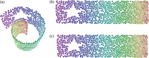
We sampled a Swiss Roll manifold, , with 2000 random points. A star-shaped region of this manifold was excluded from being sampled. We then used manifold sculpting (Gashler, Ventura, and Martinez 2011) to reduce the dimensionality of these points. Figure 12(a) shows the original points. Figure 12(b) shows the results obtained from reducing the dimensionality to 2, without using CycleCut. Figure 12(c) shows results that were obtained when CycleCut was used to preprocess neighbourhood connections. The results obtained with CycleCut were nearly identical to those obtained without it. This shows that CycleCut often has little adverse effects in cases where it is not needed. (This experiment is an example of case 3 shown in Figure 3.)

Figure 12. (a) Two thousand sample points on the surface of a Swiss Roll manifold with a star-shaped region excluded from sampling. (b) Results obtained by reducing this data set to two dimensions with manifold sculpting (Gashler et al. 2011). (c) Results obtained with manifold sculpting after CycleCut was applied. In this case, 28 neighbour connections were cut, but the results are nearly identical to those obtained without CycleCut. This shows that CycleCut has little adverse effect in cases where it is not needed.

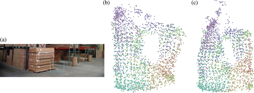
In another experiment, we simulated a robot navigating within a warehouse environment by sampling in a windowed region from an image of a warehouse (Figure 13(a)). We simulated the forward and reverse movements by changing the size of the window, and we simulated the lateral movement by moving the window horizontally. Linear interpolation was used to produce a uniform-sized view from the perspective of the simulated robot. We applied 4000 random actions from the set <texlscub>move forward (scale down the window size), move back (scale up the window size), move left, move right</texlscub> to this robot and collected the corresponding images from its view. We simulated a physical obstacle by preventing this robot from entering a rectangular region near the middle of its state space. We also injected Gaussian noise into both the transitions and the observations to simulate unreliable hardware. Specifically, we added a random value from a Gaussian distribution with a standard deviation of 5% of the channel range to each colour channel of each pixel in each observed sub-image. We also added Gaussian noise with a standard deviation of 5% of the step length to each state transition, such that the simulated robot would transition to a state only near to the one specified by the actions that it performed. After collecting 4000 observation images, we used the Temporal NLDR algorithm (Gashler and Martinez 2011) to reduce them to the corresponding estimates of the robot's position. These results are plotted in Figure 13(b). The ‘hole’ in the centre of these results indicates that the robot did not collect any observations in that region of its state space, as intended. We then repeated this experiment with the addition of CycleCut to preprocess the neighbourhood graph. The results that were obtained with CycleCut exhibited a similar overall structure, as shown in Figure 13(c). Some differences, however, appear in the upper region of this result. This occurred because that portion of the state space was poorly sampled, because the robot only wandered into that region one time, so the manifold learning algorithm had little structural information to preserve in that region.

Figure 13. (a) The image of a robot navigating within a warehouse environment that was simulated by sampling this image within a window. We simulated the forward and reverse movements by changing the size of the window and we simulated the lateral movement by moving the window horizontally. Linear interpolation was used to produce a uniform-sized view from the perspective of the simulated robot. We applied 4000 random actions from the set<texlscub>move forward, move back, move left, move right</texlscub>to this robot and collected the corresponding images. We simulated a physical obstacle by preventing this robot from entering a rectangular region near the middle of its state space. We also injected Gaussian noise into both the transitions and the observations. (b) Results obtained using Temporal NLDR to reduce these images to the estimates of the robot's position. (c) Results obtained after repeating this procedure with the addition of CycleCut. In this case, the ideal results would be unchanged. Although CycleCut did change the results somewhat, the overall structure of the state estimates is very similar whether or not CycleCut was used. The most significant difference occurs near the top region, where only a small number of samples were taken (because the robot only wandered into that region one time).

5. Conclusions

We presented an algorithm called CycleCut, which finds a minimal cut necessary to break the large atomic cycles in a graph. We demonstrated, both theoretically and empirically, that this algorithm is useful for preparing neighbourhood graphs for manifold learning. With many typical problems, neighbourhood graphs contain no large atomic cycles. In such cases, CycleCut has no effect on the results. When neighbourhood graphs do exhibit large atomic cycles, however, dimensionality reduction can be difficult. In these cases, CycleCut finds a minimal set of connections that must be cut to eliminate all large atomic cycles from the graph.

CycleCut makes existing NLDR algorithms robust to a wider range of problems. Using CycleCut to preprocess neighbourhood graphs incurs little cost because it scales well, it has little adverse effect on results in the case where large atomic cycles are expected in the neighbourhood graphs, and it guarantees never to break connectivity. When shortcut connections exist, CycleCut guarantees to remove them, and when the manifold connects back to itself, CycleCut has the beneficial effect of removing the minimal number of connections such that the manifold can be unfolded without introducing local distortions.

References

- Balasubramanian , M. and Schwartz , E. L. 2002 . The Isomap Algorithm and Topological Stability . Science , 295 ( 5552 ) 7a
- Brandes , U. 2001 . A Faster Algorithm for Betweenness Centrality . The Journal of Mathematical Sociology , 25 ( 2 ) : 163 – 177 .
- Cukierski , W. J. and Foran , D. J. Using Betweenness Centrality to Identify Manifold Shortcuts . IEEE International Conference on Data Mining Workshops . pp. 949 – 958 . 2008, ICDMW ’08
- Ford , L. and Fulkerson , D. 1962 . Flows in Networks , Princeton , NJ : Princeton University Press .
- Gashler , M. 2011 . Waffles: A Machine Learning Toolkit . Journal of Machine Learning Research , 12 ( July ) : 2383 – 2387 .
- Gashler , M. and Martinez , T. Temporal Nonlinear Dimensionality Reduction . Proceedings of the International Joint Conference on Neural Networks IJCNN’11 . pp. 1959 – 1966 . IEEE Press .
- Gashler , M. , Ventura , D. and Martinez , T. 2011 . Manifold Learning by Graduated Optimization . IEEE Transactions on Systems, Man, and Cybernetics, Part B: Cybernetics , 41 ( 6 ) : 1458 – 1470 .
- Hein , M. and Maier , M. 2006 . “ Manifold Denoising ” . In Advances in Neural Information Processing Systems , Edited by: Schölkopf , B. , Platt , J. C. and Hofmann , T. Vol. 19 , Cambridge , MA : MIT Press . http://people.kyb.tuebingen.mpg.de/mmaier/ManifoldDenoising.html.
- Nikolopoulos , S. D. and Palios , L. Hole and Antihole Detection in Graphs . SODA ’04: Proceedings of the Fifteenth Annual ACM-SIAM Symposium on Discrete Algorithms . pp. 850 – 859 . Philadelphia , PA : Society for Industrial and Applied Mathematics .
- Spinrad , J. P. 1991 . Finding Large Holes . Information Processing Letters , 39 ( 4 ) : 227 – 229 .
- Tenenbaum , J. B. , de Silva , V. and Langford , J. C. 2000 . A Global Geometric Framework for Nonlinear Dimensionality Reduction . Science , 290 : 2319 – 2323 .
- Varini , C. , Degenhard , A. and Nattkemper , T. W. 2006 . ISOLLE: LLE with Geodesic Distance . Neurocomputing , 69 ( 13–15 ) : 1768 – 1771 .
- Wei , J. , Peng , H. , Lin , Y. S. , Huang , Z. M. and Wang , J. B. Adaptive Neighborhood Selection for Manifold Learning . 2008 International Conference on Machine Learning and Cybernetics, . July . pp. 380 – 384 . Vol. 1