Genetic programming for detecting target motions

Abstract

This study presents a selective motion detection methodology which is based on genetic programming (GP), an evolutionary search strategy. By this approach, motion detection programs can be automatically evolved instead of manually coded. This study investigates the suitable GP representation for motion detection as well as explores the advantages of this method. Unlike conventional methods, this evolutionary approach can generate programs which are able to mark target motions. The stationary background and the uninteresting or irrelevant motions such as swaying trees, noises are all ignored. Furthermore, programs can be trained to detect target motions from a moving background. They are capable of distinguishing different kinds of motions. Such differentiation can be based on the type of motions as well, for example, fast moving targets are captured, while slow moving targets are ignored. One of the characteristics of this method is that no modification or additional process is required when different types of motions are introduced. Moreover, real-time performance can be achieved by this GP motion detection method.

Keywords:

• genetic programming
• motion detection
• noisy data
• machine learning
• machine vision
• evolutionary computation

1. Introduction

Detecting motions is one of the key aspects in many real-world machine vision systems as often the moving objects are more informative and more essential to understand the environment, for example, moving vehicles for traffic control systems, pedestrians for security surveillance systems and incoming objects for autonomous robots. There are a large number of motion detection methods available of which most are based on manually designed algorithms such as temporal difference and background modelling techniques (Hu, Tan, Wang, and Maybank 2004). Lipton, Fujiyoshi, and Patil (1998) used a temporal difference-based method with connected components and histogram analyses to detect moving vehicles and people. Stauffer, Eric, and Grimson used ‘N’ mixture of Gaussians to build the background model. Using this approach, they were able to ignore uninteresting motion of swaying tree branches and water ripples (Stauffer, Eric, and Grimson 2000). Haritaoglu, Harwood, and Davis used a simplistic approach in their background model, where the minimum, maximum and the maximum inter-frame difference pixel values for each pixel are captured over a training period. Any pixel that is beyond the background model by more than the threshold amount will be considered as foreground pixels (Haritaoglu, Harwood, and Davis 2000). These methods may be combined to form a motion detection module (Abdelkader and Zheng 2006), or work with other components such as object extraction module to accomplish motion detection (Huang 2011). There are also algorithms proposed based on Hue saturation value (HSV) colour space and statistics (Hu and Hu 2011). Nevertheless, these traditional methods are developed with hypotheses of how vision systems should work, such as motion being the change contrast to background. They all rely on manually designed features or modules. These features or modules not necessarily reflect the underlying mechanism of how our own biological vision system perceive and process motion information.

The approach we presented here on the contrary is based on machine learning, in particular genetic programming (GP), by which motion detection algorithms are automatically constructed based on a set of given examples. Through this method, different kinds of motion detection algorithms can be generated simply by providing different sets of given examples, without changing the methodology itself. The responsibility of this method is actually to find a suitable program to minimise the errors in detecting targets from non-targets. In the context of motion detection, the targets are moving objects. However, it is often the case that some movements are of no interest for a vision application, for example, waving trees and water ripples in security systems, pedestrians in vehicle traffic control, random motions introduced by noisy input. These motions need to be removed prior to the detection or after the detection in conventional approaches. This kind of extra process would not be required in our approach as uninteresting motions can be simply treated as the non-targets. Instead of establishing and validating a hypothesis, this approach focuses on solving the problem itself without any presumption on how a motion detection algorithm should look like. It explores possible paths to map the input, in our case the video frames, with the desired output which are areas either containing target motion or not. A successful detection program generated by GP is such a mapping function. It can generalise rules for detecting motions based on given examples. One important aspect is that the detection methods or programs or modules are not manually crafted, but automatically generated.

GP is an evolutionary machine learning algorithm inspired by the survival-of-the-fittest principle (Koza 1992). It has been proved as a powerful problem-solving paradigm in a large number of different areas (Poli, Langdon, and McPhee 2008), including image processing and machine vision. For example, Poli (2000) used GP to evolve programs for detecting blood vessels from X-ray coronarograms. Similarly, he evolved GP programs which could perform image segmentation on brain magnetic resonance graphs (Poli 2000). In Lin and Bhanu's (2005) work, GP programs were trained to identify various targets such as road, lake and field regions from synthetic aperture radar images. Zhang, Ciesielski, and Andreae (2003) were able to generate object detection programs by GP to classify haemorrhages and microaneurisms in retina images. Song and Ciesielski (2008) evolved GP classifier for texture classification and segmentation. Howard, Roberts, and Ryan (2006) applied GP for vehicle detection, which was to find vehicles in infrared line-scan images taken from various industrial, urban and rural environments. Trujillo and Olague (2008) and Olague and Trujillo (2011) generated image operators to detect interest points based on GP. Larres, Zhang, and Browne (2010) used GP to generate image classifiers and Liddle, Johnston, and Zhang (2010) used it to evolve object detection programs. Ebner (2010) also reported GP-generated object detectors. Most of these works have shown that the performances of these automatically generated solutions evolved by GP are at least comparable to the manually coded programs.

1.1. Goals of this study

The aim of this article is to present the framework of this motion detection method to study the advantages of this approach. The specific goals of this study are the followings:

•	how motion detection problems can be represented in GP so that effective detectors can be automatically generated by the evolution process without relying on manually crafted features or conventional image processing operators;
•	how this GP method would perform especially when unwanted motions are present;
•	how this GP method would distinguish objects travelling with different speeds.

This article is structured as follows: Section 2 describes the basics of GP. Section 3 gives an overview of the methodology. Section 4 discusses a few representations for motion detections along with the experiments on them. Section 6 reports the investigation on motion detection from unstable background. Section 7 presents the study on differentiating motions with various speeds. Following these experiments, Section 7 discusses this GP approach in more detail. Section 8 concludes this article.

2. Background of GP

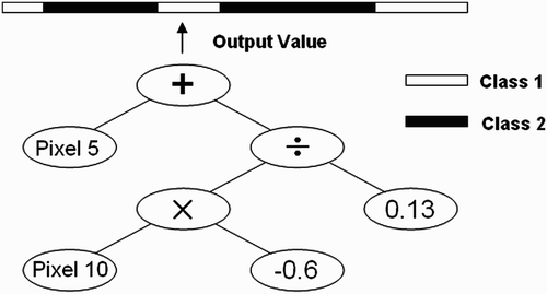
The basic representation of GP is tree structure programs as illustrated in Figure 1. The operators of the programs are those internal nodes on the tree such as + and −, while the operands are the leave nodes. In GP terminology, internal nodes and leave nodes are called functions and terminals, respectively.

Figure 1. A sample GP program tree.

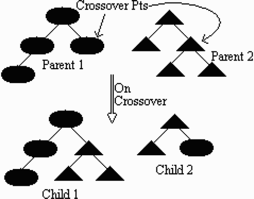
Similar to that in the biological world, a GP evolution process consists of many generations. The initial generation is a group of GP programs which are randomly generated. Each program will be evaluated in terms of the performance on solving a particular problem using the fitness measure/function. In our case, it is the performance on motion detection. Programs with a better fitness have a higher probability to be selected for reproducing the next generation. There are several ways to create a new generation from the chosen programs in the current generation. Crossover is one of them, a pair of selected programs exchanging their subtrees at random positions to result two new programs (as seen in Figure 2). Mutation is another, one selected program replacing its one subtree with a randomly generated subtree to result in a new program (as seen in Figure 3). In addition, a selected program may be directly cloned into the new generation. This is known as elitism. Programs in the new generation will be again evaluated with the same fitness measure. Fitter ones will survive for reproducing offspring in the next generation. Supposedly, the fitness of the best offspring in the next generation would be better than that of the previous generation. This evaluation–selection–reproduction process is iterative and will continue until one of the termination conditions is met, for example, a perfect program is found or the maximum number of generations is reached.

Figure 2. Crossover operation.

Figure 3. Mutation operation.

For the task of motion detection, a GP program is a detector which is effectively a classifier, classifying target motions from the negatives. A program is evaluated from the bottom of the tree to the top. The inputs are passed to the programs through terminals, the leave nodes, and consequently processed by the functions, the internal nodes. The final output from the root node at the top is a numeric value, which is then interpreted as the decision. One way of interpretation is treating values larger than zero as positives, meaning target motions, and other values as negatives. Another way is dynamically segmenting the numeric spectrum into multiple sections for both positive and negative classes as illustrated in Figure 1, for example, positives are values in the two ranges coloured in white and negatives are values fell into the black ranges. This method is called dynamic range selection (Loveard and Ciesielski 2001). Previous work on evolutionary motion detection can be found in Song and Fang (2008), Pinto and Song (2009), Song and Pinto (2010) and Shi and Song (2011).

3. Methodology

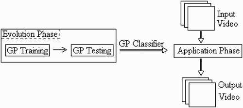
The overview of our methodology for motion detection is shown in Figure 4, which consists of two main components: the evolution phase and the application phase. The first one is to generate the detection program, while the second is to apply the best program evolved from the evolution phase to video streams. The evolution phase itself has two parts: ‘training’ and ‘test’.1 The former is basically the evolutionary process during which detection programs are generated and evolved on training instances. The latter is to evaluate individual detectors obtained from training against some unseen data. The detector which achieved the highest accuracy in the test will be deployed in the application phase. More details of each phase are given in the following subsections.

Figure 4. Methodology overview.

3.1. Evolution phase

As mentioned before, GP programs are evolved during this phase as classifiers, which can differentiate target motions from all negatives including stationary background and motions that are not interesting. To enable the evolutionary process, a data set is needed here which consists examples of input and the corresponding output. An input is a 20×20 two-dimensional (2D) array taken from video frames at different positions. If the majority of the pixels in that 20×20 input are labelled (by human) positive, then that is considered positive. Alternatively, it is considered negative. They are the correct answers that GP programs are trained to match with. The actual values stored in this 20×20 matrix depend on how the frames are represented. Different representations are discussed separately at the end of this section. The size of the matrix has no particular significance, but an empirical choice. Obviously, large sizes require more computational resource, while a small window size may not contain sufficient amount of information to enable accurate detection.

The labelled data collection is divided into two sets: the training set and the test set, one for the training part and the other for the evaluation of trained GP programs. The best achiever on the test set is selected for the application phase. Note that the training and test sets are sampled only from a small proportion of one video. The video data in the application phase are generally unseen during the evolution phase. Typically, we collect 900 positive and 1800 negative samples to form the data set. In general, there are many more negatives than positives as moving targets usually just occupy small parts of one frame. Most of the negatives are removed to avoid a largely unbalanced data set. From the data set, 300 positive and the equal number of negative examples are used for training and the rest for testing.

The fitness measure in the training and the performance indicator in test are the same, simply the classification accuracy on given input, as shown below:

where TP is true positive, the number of correctly identified positives, and TN, true negative, is the number of correctly classified negatives. The total number of examples in the data set is TOTAL. Obviously, a higher accuracy will result in a better fitness value.

Table 1 provides the runtime parameters for the training process presented in this study. The number of individuals in each generation, population size, is set to 30. The minimum depth of GP tree is 2 as a single-node program would not be any good. The maximum depth of tree is set as 9 to prevent over-sized programs. The percentages of individuals generated by mutation and by crossover are at 5% and 85%, respectively. The rest 10% of the individuals are copied from the last generation by elitism. This relatively low mutation rate is consistent with that in other image-related GP applications reported in the literature as higher mutation rates often resulted in lower fitness. The max generation is 300 in most of the experiments, but 150 in some experiments. These parameters by no mean are the best combination, but empirically suited for this particular problem.

Table 1. GP runtime parameters.

Population size	30
Maximum depth	9
Minimum depth	2
Mutation rate	5%
Crossover rate	85%
Elitism rate	10%

3.2. Application phase

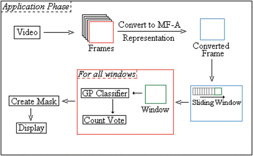
A program with the highest test accuracies from the evolution phase is ready to be applied onto videos. However, by itself, it is not directly suitable for performing motion detection tasks as it operates on a 20×20 input, which is too small to contain a video frame and too coarse to mark the contour of a moving target. Instead, the detector program is fed into a process as shown in Figure 5.

Figure 5. Overview of the application phase.

First, a video clip or live video stream is transformed into one of the multi-frame (MF) representations by functions, which are discussed in Section 4, to generate pseudo-frames or converted frames. Then, a sliding window of size 20×20 will sample sub-images from each pseudo-frame starting from the top-left corner to the bottom-right corner with a certain interval. At each window position on that frame, the GP program will take the 20×20 pixels under that position as the input and classify it as either containing a target motion or not. If the output of the program at that position is positive, then all the 400 pixels under that window position are marked as positive. The same applies for negatives.

The key part in the application phase is voting. Obviously, if the interval between consecutive window positions is smaller than 20, then there will be overlaps among them. Consequently, one pixel will appear in multiple window positions and classified multiple times. For each pixel, all its class labels generated by different windows over it are recorded. The final class of this pixel is determined by the votes. It would be marked as a part of the moving target if the majority of the sub-images containing this pixel are identified as positives. This interval is adjustable to suit the need of an application. A wide gap would result in fast execution, while a narrow gap would produce smoother contour of the output. The experiments presented here all used 8 as the shifting distance between two adjacent window positions.

From Figure 5, we can see that this approach does not require additional pre-processing or post-processing such as image sharpening and noise reduction, which are often required in conventional machine vision methods.

4. Representations

A suitable representation is critical for any search problems. There is no exception here as fundamentally GP is a search strategy to find a program which is expected to solve the problem. In the context of motion detection, there are two aspects of representations. One is how to define operators (functions) and operands (terminals) on a GP tree. The other is how to represent video frames so GP programs can process them. They are discussed and experimented in the following subsections.

4.1. Function sets

The operators listed in Table 2 show three function sets, separated by horizontal lines. Along each operator, the data type of its return value and the data type of its arguments are given in the table. ‘Double’ refers to double-precision floating-point numbers. ‘Boolean’ simply is a Boolean value, either true or false.

Table 2. Three function sets.

Function	Return type	Arguments
Basic
+	Double	Double, Double
−	Double	Double, Double
×	Double	Double, Double
/	Double	Double, Double
=	Boolean	Double, Double
<	Boolean	Double, Double
>	Boolean	Double, Double
if	Double	Boolean, Double, Double
AMM: Basic + the following three
AVG	Double	4× Doubles
MAX	Double	4× Doubles
MIN	Double	4× Doubles
sAMM: Basic + the following three
statAVG	Double	6× Doubles
statMAX	Double	6× Doubles
statMIN	Double	6× Doubles

The first set is named as the ‘Basic’ function set. It only contains simple arithmetic operators and logic operators such as addition, subtraction, multiplication and protected division (division by zero results in zero). The ‘if’ operator requires three arguments and returns the second argument if the first argument is true, or return the third argument if the first argument is false. The first argument of the ‘if’ operator requires Boolean operators ‘equal to’, ‘greater than’ or ‘less than’ to feed a true/false value.

The second set is named as ‘AMM’ because it contains three extra image operators ‘AVG’, ‘MAX’ and ‘MIN’. These functions sample an area out of the 20×20 input image and then calculate the average, minimum and maximum pixel values of that area. These functions have four arguments which are basically coordinates. Two of them define the top left position of the sampled area, while the other two indicate the bottom right corner of it. These four arguments will be modularised before sampling pixel values, so the coordinates will be in between [0, 19]. These functions are to capture localised features under the sampling window position, especially when the prominent motion information is in smaller local regions, rather than in the entire input. Additionally, calculating the average, max and min for the entire 20×20 window would be much more costly than doing that for a smaller area. It is expected that the optimal regions can be defined by the GP evolutionary process.

The third set (referred as the ‘sAMM’) includes three additional functions statAVG, statMAX and statMIN, which are the variation of the functions in set ‘AMM’. Instead of calculating the average, maximum and minimum values over a region, the calculation here is just based on six arguments of these functions. These arguments directly take pixel values as inputs. Compared with the operators in AMM function set, the computational costs of these functions are much less as they do not require all the pixels in the sampled area although it would be smaller than 20×20. Moreover, there are more flexibility in ‘sAMM’ functions as they can select pixels across the entire input image, rather than pixels confined in a specific region. Our earlier studies have shown that successful programs evolved by GP often only involve a handful of input variables to perform a particular task, including image-related classification problem (Zhang, Andreae, and Pritchard 2003). It is expected that GP can find a few key points which are sufficient to distinguish target motion from everything else. Hence, there is no need to include all pixels. In comparison, conventional image operators which are often not selective as they process all pixels on an input image. Note that it is possible to introduce more or less than six arguments for these functions. The choice of six here is based on early empirical study on the balance between performance and computational cost.

The function nodes in the above function sets are all simple operators such as arithmetic operators, logic operators and simple pixel aggregation operators. No complex or conventional image operators are used as the expectation is that the evolutionary process would be able to utilise these simple operators to form programs suitable for a particular problem, since complex image operators are just some combinations of simple operators. Moreover, complex operators are usually computationally expensive, hence not good for the real-time performance.

4.2. Terminal set

The choice of program operands for motion detection is straightforward. As given in Table 3, the terminal set only contains two types of operands. The first type generates random numbers between 0 and 1, which would behave like coefficients in formulae. The second type is input nodes which read data from the 20×20 pixels sampled from a pseudo-frame, which is discussed in the next subsection. The index [x] corresponds to the position of that pixel on the sub-image. An important aspect is that a 2D 20×20 sub-image is represented here as a one-dimensional (1D) array which contains 400 elements. In this study, all image pixels are converted into greyscale as that is the common practise although colour can be easily handled as well.

Table 3. Terminal set.

Terminal	Return type
Random	Double
Pixel[x]	Double

4.3. Frame representations

In tasks such as image classification, edge detection, texture classification, a static image can be directly fed into GP programs. However, one single image sampled from video sequences is not sufficient to capture motion information. Therefore, MFs should be represented in the input. Consecutive frames can be combined into a pseudo-frame, which retains pixel variations over this series of frames. Three different ways of generating pseudo-frames are proposed below, which are referred as ‘MFA’, ‘MFB’ and ‘MFC’, respectively.2

The first one, shown in Equation (2), keeps the temporal difference over a sequence of frames. In the equation, ‘n’ is the number of frames in the sequence, x is one pixel position using 1D index. Similar to input terminals given in Table 3, 2D images are viewed as 1D arrays. The function I(x, i) returns the intensity value of pixel x at ith previous frames. The output is the aggregated difference between pairs of consecutive frames over ‘n’ number of frames.

Equation (3) is the second representation, MFB(x). This is a simpler form of calculating variations between frames, without using absolute differences. It only compares the latest one and the earliest one in a series of frames, and ignores the frames in between as (A−B)+(B−C) is equivalent to A−C. This representation is expected to be more efficient as the computational cost is low. Since the difference could be a negative value, so this representation is expected to somehow capture the direction of movement. Negative values are not in MFA (Equation (2)).

The third one is MFC(x), by which a pseudo-frame is represented in Equation (4). There is a weight component, n−i, in the formula to indicate the ‘age’ of a frame. More recent frames result in higher weights. The frame immediately precedent to the current one receives a weight n−0=n, while the oldest frame in the sequence only receives a weight n−(n−1)=1. Similar to MFB(x), there is no absolute value in this formula.

In the following investigation, the size ‘n’ used by all representations is consistently 3.

4.4. Experiments

This section shows all the experiments with the presented methodology. All videos are taken with non-professional camera under arbitrary conditions. All the videos are unprocessed. Such an approach is to remove the possible human control factors as in the real-world application, the method should not tie to a particular setting, but be general.

4.4.1. Frame representations

To study the suitability of each frame representation MFA, MFB and MFC, we tested them on a real-world scenario, which is to detect moving vehicles on streets. The results are presented in Figure 6. The X-axis of these figures is the number of generations and the Y-axis is the detection accuracy. The solid lines illustrate the best training accuracies achieved during these GP runs, while the dashed lines on the same graph are the corresponding test accuracies. Each experiment is repeated at least 10 times, the results shown here are the averages.

Figure 6. Comparing three MF representations in the evolution phase.

The results clearly show that MFA outperforms both MFB and MFC, in training and in test. When applied in the application phase, detectors using the MFB and MFC representations generate less true detection but more false positives, compared with those in the MFA representation. Such results indicate that absolute difference used in MFA is beneficial. The investigation discussed in the later sections uses the MFA representation.

4.4.2. Function sets

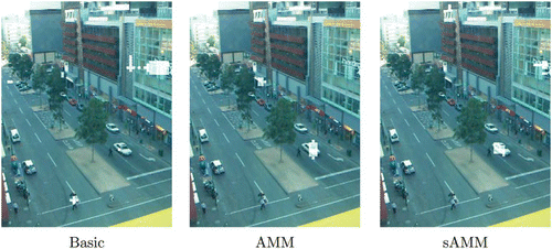
The second part is to determine the suitable function set, either Basic or AMM or sAMM. Figure 7 shows the average training and test accuracies over 10 runs on a moving vehicle detection problem. Instead of setting the maximum generation at 150 as shown in Figure 6, the maximum here is 300. Although the maximum generation is doubled, the difference of training performance between Basic, AMM and sAMM is not very obvious. The training and test accuracies of Basic is slightly lower, while those of AMM and sAMM are quite comparable, as shown in Figure 7. However, the difference between them in the application phase is much clearer as shown in Figure 8. The task itself is to identify moving vehicles while ignoring background such as parked vehicles as well as other moving targets such as pedestrians. The targets detected by the GP programs are marked with a white mask. The three images in the figure are the results from the three classifiers on the same video frame. Classifiers in AMM and sAMM detected the moving white car while ignoring the parked vehicles and pedestrians. However, the classifier using Basic function set did not mark that white car, but gave false positives on one pedestrian and on a building. Applying these three function sets onto other scenarios results in similar outcomes. In the investigation discussed later, sAMM is used since it is computationally more cost effective compared to AMM.

Figure 7. Comparing three function sets in the evolution phase.

Figure 8. Comparing three function sets in the application phase. Source: Photograph by the author.

5. Environment with non-stationary background

The focus of this section is to show how well this GP method could handle applications with non-stationary background, as that often occurs in real-world scenarios. The first problem is to detect cruising boats on a river. The motion from the ripples and the waves behind a moving boat should be ignored as the only interesting targets are the boats. The second problem is to detect moving vehicles on streets while ignoring pedestrians and swaying trees. The third one is still to detect vehicles but from a moving camera. The motion introduced by the camera movement should not affect the detection. Furthermore, raining condition and artificial noise are introduced to further complicate the situation. Additionally, a traditional method, background modelling, is applied on the same videos for comparison.

5.1. Boat detection

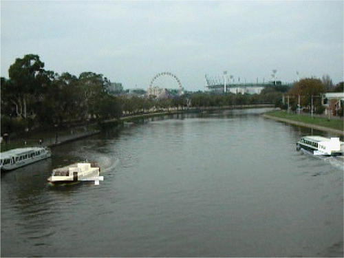
Table 4 lists the training and test accuracies with the corresponding TP and TN rates from the evolution phase. The GP classifiers here are evolved specifically for this scenario, but tested on unseen video frames. Figure 9 shows a sample output frame from the application phase. The uninteresting motions on rivers surface are not marked and only the moving boats are correctly highlighted.

Figure 9. Detecting moving boats. Source: Photograph by the author.

Table 4. Training and test results for detecting moving boats.

	Accuracy (%)	TP (%)	TN (%)
Training	94.18	98.67	89.70
Test	88.51	93.91	83.11

5.2. Vehicles detection

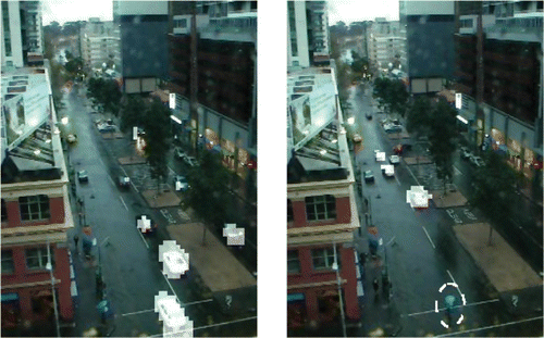
Similar to Table 4, Table 5 lists the accuracies obtained from the evolution phase in a vehicle detection problem. Figure 10 illustrates the outcome from the application phase in which the program with the highest test accuracy is applied onto two unseen video frames. It can be seen that the background contains waving trees and pedestrians (circled in the graph). Despite the un-stationary background, thorough and consistent detection is achieved by the GP program. Only the moving cars are marked by the GP program. Car parked along the streets and cars stopped on the road are not marked by the GP program. The vehicle located at the right bottom of the left figure is partially marked as it just starts to move forward.

Figure 10. Two sample output frames from the moving vehicle detection scenario (sunny day). Source: Photograph by the author.

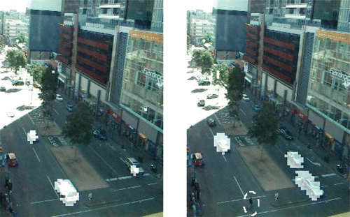
Table 5. Training and test results for detecting moving vehicles.

	Accuracy (%)	TP (%)	TN (%)
Training	99.83	100	99.67
Test	99.09	99.56	98.63

5.3. Moving camera

The videos, here, are taken from a moving camera just like that in some surveillance systems, which pan the camera through one corner to another to cover a wide area. Every pixel, either in the background or in the foreground, changes over frames. We have tried by directly applying the best classifier trained previously in Section 5.2 on these videos. Unsurprisingly, the performance is very poor as the training data there do not contain examples of camera movement. To handle this new situation, new classifiers are trained specifically. The results from the evolution phase are listed in Table 6 and sample outputs from the application phase are shown in Figure 11. Clearly, the motion from camera did not affect the overall performance. The pedestrians and parked cars are also correctly ignored in this case. Compared with previous experiments, the methodology remains unchanged. The only difference is just the training data.

Figure 11. Two sample output frames from the moving camera scenario. Source: Photograph by the author.

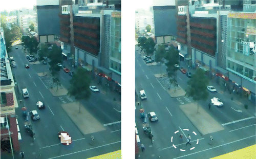
Table 6. Training and test results for moving camera scenario.

	Accuracy (%)	TP (%)	TN (%)
Training	100	100	100
Test	99.33	99.29	99.37

The moving camera did not only introduce wholesome movement on the frames, but also brought an additional complication, the variation in illumination conditions. It can be seen from Figure 11 that the left frame is darker than the right frame due to different camera angles. However, that variation did not affect the performance of GP programs.

5.4. Raining condition

Raining condition often occurs in outdoor applications. A reliable system should be able to handle the complications caused by rain. One approach in our GP method is to re-train a GP program for raining condition similar to what was done for the scenario of moving camera. However, camera movement is controllable, but not the weather conditions. If we have multiple programs trained for different weather conditions, then an additional weather detection process is required to allow switching between programs. It would be ideal to have one program which can handle multiple conditions. Therefore, we directly tested the program trained for moving vehicle detection presented in Section 5.2 on a rainy day. The training data for this program were collected on a sunny day.

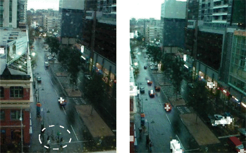
The results are shown in Figure 12 of which the images are very different from that in Figure 10, Section 5.2. The images are much darker overall but with brighter road surface caused by reflection. Rain drops constantly blend in the scene to blur the images. However, no obvious detrimental effect can be observed as the moving cars are all marked and the pedestrian is ignored. The headlights of the coming cars actually made the detected areas much larger than the vehicle itself as the lights and the reflection were considered positive as well by the GP program.

Figure 12. Two sample output frames: vehicle detection under raining condition. Source: Photograph by the author.

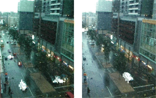
Similarly, the program evolved for the moving camera scenario in Section 5.3 is directly applied on a rainy day video as well. The results are shown in Figure 13, which presents similar outcome to that in Figure 12. This GP program is able to directly handle the rainy input without compromising the performance too much despite of the difficulties such as motions introduced by rain drops, darker environment and reflection from the wet road surface. A group of pedestrians crossing the road (circled) are again not marked.

Figure 13. Two sample output frames: moving camera scenario under raining condition. Source: Photograph by the author.

5.5. Noises

Noise is another potential problem for real-world vision applications. They may be caused by various unpredictable reasons such as faults in the sensor itself or fluctuation in power supply. Therefore, noise is also included in this investigation. First, the program trained for the moving camera scenario presented in Section 5.3 is again directly applied to noisy videos. The first video is taken from a moving camera on a sunny day, same as that in the training. However, Gaussian noise of variance 30 is added into this video. The second video is also taken from a moving camera, but on a rainy day. Gaussian noise of variance 30 is also added. Note that these noises are randomly injected into each frame. No pair of consecutive frames contains the same noise, so these noises do cause large variations in pixel values.

The results from these two videos are illustrated in Figures 14 and 15. Note that this detector was trained only for a sunny day without any artificial noises. However, this GP program is able to perform reliably and consistently. It seems capable of handling a rainy condition, additive noises and the combination of these two. Neither adjustment on the methodology nor the re-training process is needed.

Figure 14. Two sample output frames: moving camera scenario with additive noise of variance 30. Source: Photograph by the author.

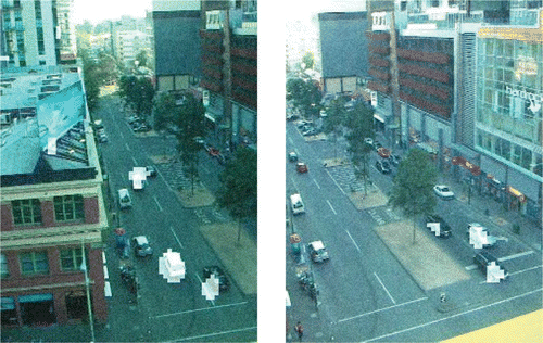
Figure 15. Two sample output frames: moving camera in rainy conditions with additive noise of variance 30. Source: Photograph by the author.

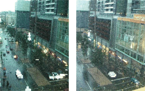
This program does have a limitation. Its performance drops dramatically when the noise level is increased beyond a variance of 30, resulting in a significant increase in false positives. This is not unexpected since no noisy data were introduced in its training data. By providing noisy data for training, GP program can handle the noise level as high as variance 50. Figure 16 shows output frames on applying a program trained with noisy data (variance 50) on a video taken by a moving camera in a rainy day, and with noise of variance 50 added. This detector is still able to perform reliably. As illustrated in the figure, the image quality is rather poor with this high level of noise.

Figure 16. Two sample output frames: moving camera in rainy conditions with additive noise of variance 50. Source: Photograph by the author.

If we further push the noise to a level beyond variance 50, then the amount of false positives increases exponentially. Such outcome suggests that, although a detector can be trained at high noise levels to handle noisy videos, the tolerance of this method to noise is not unlimited. The accuracy diminishes rapidly. Even for human eyes, videos with noise level higher than 50 are not easily recognisable.

5.6. Comparison

The previous results show that the GP method is able to generate reliable detection programs, which can cope up with different environments without re-training. In this part, the background modelling approach is applied onto the same data for comparison purpose. As suggested by Haritaoglu et al. (2000), that is, this approach uses the minimum, maximum and maximum inter-frame difference of pixels to model the background.

5.6.1. On handling uninteresting motions

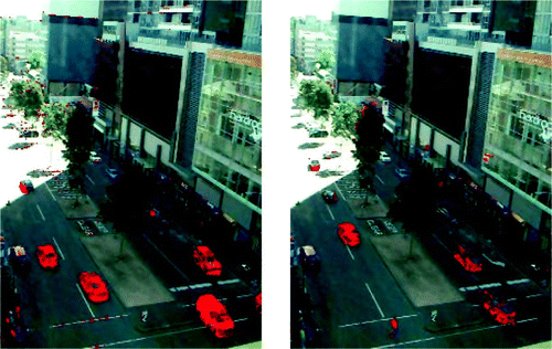
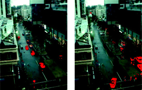
Figure 17 shows the output resulted by the background model on a fixed camera under a bright sunny condition. Figure 18 shows the results of the same method, for videos taken from a fixed camera under a rainy condition. The detected area is marked in solid red colour to make it easier to compare with the results from the GP method. From the figures, we can see that, although most of the moving objects are detected, the uninteresting movements such as the pedestrians are also highlighted. Such outcome is not a surprise because the background modelling method cannot establish a suitable model to differentiate various motions in the foreground.

Figure 17. Output frames by background modelling, on a fixed camera, trained and applied on a bright sunny condition. Source: Photograph by the author.

Figure 18. Output frames by background modelling, on a fixed camera, trained and applied on a rainy condition. Source: Photograph by the author.

5.6.2. On handling noises

As seen previously in Figures 14–16, GP motion detectors are able to handle additive noise of variance 30 without seeing noisy data in the training. However, that is difficult for the background modelling. Figure 19 illustrates that point. The left figure shows the result of applying a model trained on no-noise data on videos with noise (variance 30). The model generates a large number of false positives. If the model is trained on the video with the same amount of noise, then this approach can achieve reasonable detection as shown at the right of Figure 19. A Gaussian noise level at 30 is applied to both of the training and the test data there.

Figure 19. Comparison between models trained on (a) no-noise data and (b) on noisy data. Source: Photograph by the author.

5.6.3. On handling unseen background

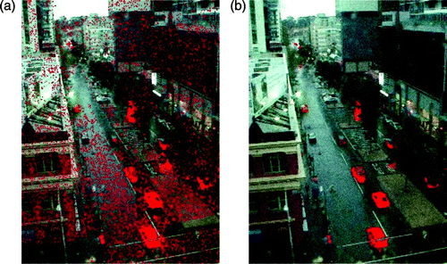
Background modelling methods train and test based on the same background. This is the case for results shown in Figures 17–19. Because these models are background specific, they would fail completely if they are applied onto a unseen environment even there is only a slight different between the new background and the background in training. Figure 20 illustrates that effect. The left image is the result of applying a model trained on a sunny condition to a video taken at a rainy condition. The right one is what happens when applying that model onto a video taken under the same lighting condition as the training video but from a slightly different angle. The false positives in both cases are simply too great to make the result of any use. Note that the camera position is fixed in these experiments. A moving camera would make the result even worse as there are no two frames having the same background in a moving camera scenario.

Figure 20. Applying background models on unseen environments: (a) unseen rainy conditions and (b) changed camera angle. Source: Photograph by the author.

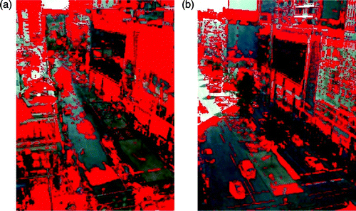
The problem of changing background (as illustrated in Figure 20) could be addressed by an appropriate image registration algorithm or SDG models suggested by Ren, Chua, and Ho (2001). However, these algorithms would require extra processing and additional computational costs. Furthermore, the performance of the model based on such registration algorithms would greatly depend on the performance of the image registration algorithm. The overall methodology would be much less generalisable. In contrast, the evolutionary motion detection method does not require any additional component to deal with these kinds of variations.

6. Differentiating targets based on speed

The previous section demonstrates the capability of GP programs in differentiating moving targets from other types of motions. In this section, we extend the study a little further to distinguishing the same type of targets but with a different speed. We like to see whether GP is able to capture object moving at a relatively high speed but ignore the same object travelling relatively slowly. A typical application scenario would be monitoring systems where fast moving objects such as a running person, a speeding car should receive more attention. The only way to differentiate target and non-target motions in this kind of applications is the speed. With the GP approach, an extra step of measuring speed would not be necessary.

6.1. Detecting faster objects

The first set of experiments is illustrated in Figure 21, which is an indoor setup, two ping-pong balls rolling from left to right. These two balls are identical in size and colour. The ball further away from the camera slides from a less steep slope on the left, hence is slower. The results from the application phase are presented in Figure 21. The detection in this section is marked in light green.

Figure 21. Sample output of detecting fast moving objects – ping-pong balls. Source: Photograph by the author.

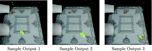
The slow moving ball is completely ignored when the fast moving ball is consistently marked as positive. There are a few tiny positive areas in ‘Sample Output 1’ at the upper left corner. They are not false positives, but genuine fast motions introduced by the operator's hand. It should be pointed out that these balls are NOT moving at a predefined speed, both in training and application. The fast ball in different videos actually travel at a slightly different speed. That is the case for the slow ball as well. The speed is even not consistent on a same video. Naturally, the balls slow down towards the end of the table. However, the important thing is that the difference in travelling speed, between ‘fast’ and ‘slow’, remains obvious to human observers who will also label the training data. So, we know GP is not based on ‘measuring’ the speed, but based on the difference in speed of positives and that of negative targets. The recognition is not specific to one speed, but a ballpark of it. This feature is important and desirable in real-world applications because pre-defining the exact speed of a moving target as the decision boundary is difficult if that is not totally impractical.

To further test the evolved detectors, they are directly applied on an outdoor scenario where cars are travelling at different speed (Figure 22). The GP detector here is not trained on cars but on ping-pong balls discussed previously. From the results, we can see the white minibus which is faster is consistently marked as green on every frame. The red sedan which is slower is ignored across the entire video. There are no other moving objects.

Figure 22. Sample output of detecting fast moving objects – vehicles. Source: Photograph by the author.

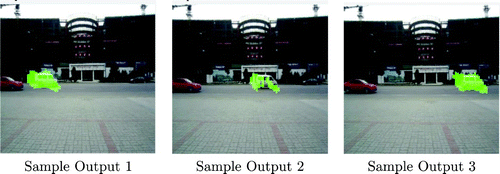
The accuracies in the evolution phase of training this detector is always 100% which triggers earlier termination. It seems that differentiating motions based on speed can be easily handled by GP.

6.2. From a moving camera

Differentiating targets based on speed is also tested on moving camera scenarios. The previous experiments involving a moving camera actually use a tripod on which the camera can pan from side to side. So only does the view angle change. However, the camera in this set of experiments is handled with no tripod. It swings from one corner to another with a small degree of free up-and-down movement. We deliberately introduce this complication, so the movement of camera would not be predictable. The combination of view angle change and position change in the camera makes the problem more difficult compared with the two previous experiments. Similar to them, the positives here in the training data are fast moving vehicles and everything else is negative.

The best classifier evolved for the ping-pong ball has been directly used on the video here. Unsurprisingly, the performance was not comparable to those shown in Figures 21 and 22. There was no TPs reported at all but with a few false ones. It seems that a new detector should be trained for this scenario to handle the higher complexity of this task.

The results of the newly trained detector from the evolution phase are listed in Table 7. That from the application phase is shown in Figure 23. In this scenario, there is a traffic light (not appeared in the video) at the right end of the frame. Vehicles slow down when they approach towards the right, for example, the bright red car. When this red car enters the scene, it is detected. However, no positive is reported on this car when it reduces its speed for the red light. There is a dark red car showing in ‘Sample Output 3’. It is ignored by the detector because it moves very slowly towards the traffic light. However, a white van (on Output 2 and 3) is consistently detected because it did not slow down, but tried to make a right turn at the corner.

Figure 23. Sample output of detecting target from a moving cameras. Source: Photograph by the author.

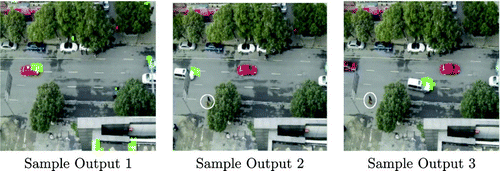
Table 7. Training results for detecting target from a moving cameras.

	Accuracy (%)	TP (%)	TN (%)
Training	92.37	96.95	87.79

All the positives, for example, the fast moving vehicles are correctly marked by the detector. Meanwhile, the negatives including the background, the parked cars and the slow moving cars are correctly ignored. Interestingly, there are two pedestrians entered the scene as well (circled in Outputs 2 and 3). The GP detector correctly considered them as negatives. This scenario can be considered as the combination of previous tasks: detecting different types of targets, distinguishing the same target with different speeds, and handling camera movement.

The results shown in Figure 23 are good but apparently not perfect. Some false positives marked on the edge are noticeable (for example, in Output 1). A possible cause is the changing perspective of the camera. For example, the left side of a cubic would not appear on camera if the camera facing the cubic is on the right side, but it will show when the camera shifts towards the left. The gradual appearance of this surface might be considered as motion by the detector. We will investigate that effect in our further work.

7. Further discussions

Through the previous sections, we illustrate how well the evolved GP programs can perform motion detection under various situations. The discussion here is on other aspects of our approach.

7.1. Execution speed

First, these evolved programs are not very big. Two example classifiers for detecting moving vehicles are shown in Figures 24 and 25, one for a fixed camera view point as in Figure 11 and one for moving camera as in Figure 13. The size of these two programs are 112 nodes and 58 nodes, respectively, including all the operators and operands. As they do not contain any loops, the computational complexity of them is as low as linear. That is important for applications which requires real-time execution and applications on devices with limited computing power. The program size is quite typical in our experiments. There are hardly any programs larger than 200 nodes.

Figure 24. An evolved classifier for detecting moving vehicles.

Figure 25. An evolved classifier for detecting moving vehicles from a moving camera.

The size of evolved program size seems to have no direct correlation with the difficulty of the task or with the detection accuracy of the program. A larger program is not necessarily superior. The detector in Figure 24 is bigger than that in Figure 25, but incapable of handling camera movement. One cause is the well-known phenomena in GP, bloat problem. Programs tend to be bigger than what is necessary due to the existence of redundant components on the tree (Kinzett, Johnston, and Zhang 2009). In this study, the focus is not on size control. So no bloat combat method is applied.

Due to the small program size and low complexity, the evolved detectors can achieve fast execution. Table 8 lists a summary of typical frame rates for two frame sizes achieved in the application phase. All the three function sets ‘sAMM’, ‘Basic’ and ‘AMM’ discussed in Section 4 are included in the table. The second column ‘Nodes’ of the table lists the size of the corresponding GP classifier. The fourth column ‘frames per second’ (FPS) is their processing speed, measured on a machine with 2.67 GHz Celeron CPU and 1 GB RAM. The raw input frame rate is the PAL/SECAM 25 FPS.

Table 8. Typical frame rates of different motion detectors.

Function set	Nodes	Frame size	FPS
sAMM	58		26
			15
Basic	28		30
			18
AMM	30		8
			13

As suggested in Table 8, these GP programs can achieve the real-time performance. Using an individual evolved with ‘sAMM’ function set (the same program with 58 node shown in Figure 25), detection could be made at 26 FPS on sized frames. In comparison, program using the ‘AMM’ function set is much slower because the operators such as AVG calculate all pixels in the sub-regions, while the operators in ‘sAMM’ only take six pixels. So, the computational cost required by ‘AMM’ is higher. In comparison, the function set ‘Basic’ provides fast execution but compromises detection performance. Therefore, ‘sAMM’ is a more suitable choice. Nevertheless, all three function sets are not computational expensive. It should be mentioned that the real-time performance does not necessarily mean a FPS higher than 25. Often, there is no need to process every single frames. A lower FPS detector could still produce the real-time output.

7.2. Program comprehensibility

One issue embedded in GP is the understandability of these evolved programs. Two examples are shown in Figures 24 and 25; however, it is difficult to reveal the underlying algorithms expressed in them. How does the program in Figure 24 ignore pedestrians? How does the program in Figure 25 compensate camera movement and noises? These are very interesting, but unanswered questions. In our future work, we would like to use simplified or synthetic problems to analyse the behaviour of the evolved motion detectors.

7.3. Differentiating types of motions

As illustrated in Section 6, GP programs can be trained to distinguish fast moving targets from slow ones and the background. However, the possibility of what kind of detectors can be evolved is not unlimited by the current methodology. For example, if we separate objects into three categories: stationary, slow and fast, then train GP programs to only pick up the slow ones, then GP cannot generate satisfactory results. This task is actually a multi-class classification problem, rather than a binary classification problem for which our current GP method is designed.

Additionally, directions cannot be used as a deciding factor. Differentiating objects moving horizontally and objects moving vertically cannot generate a satisfactory result. In our investigation, we find that direction is irrelevant to these GP motion detectors. Although generally a motion detection method is not required to be sensitive to the direction of the motion, in reality there might be situations that one direction is more interesting than others, such as incoming traffic towards a security gate is more important than outgoing traffic. To handle the directional information, we investigate a different representation scheme as the current MFA representation does not generate values below zero. So, it does not give directional information. In the meantime, other representations not using absolute values (MFB and MFC) do not produce good detectors. Furthermore, a frame is regarded as a long 1D array, rather than a 2D matrix in our representation, so the spatial relationships between pixels are somewhat lost.

8. Conclusions

In summary, a methodology of automatically constructing motion detection programs is presented in this article. This method is based on GP which is an evolutionary search strategy. In addition to describing the overall framework, various representations including function sets and MF schemes are investigated. A suitable set of representations are suggested and tested in various scenarios where unwanted motions also appear in the same scene, such as detecting moving boats where ripples exist; detecting moving vehicles where pedestrians and swaying trees exist; detecting genuine target where the camera itself is in motion. In addition, the method is tested on scenarios where speed is the indicator. Programs are evolved to recognise fast moving target and ignore the background and the same target which moves in a much lower speed. This article also discusses the execution time of these evolved programs and other aspects of the methodology.

In conclusion, the method of evolving motion detection program by GP is general and can be applied onto various applications without modification on the methodology, but providing suitable data set for program evolution. It is able to generate programs that cannot only ignore background but also differentiate target motion from other types of motion, being a different moving object or the same object moving slowly, if examples of the positive and the negative are given for training. The trained programs by the GP approach are quite reliable. They are able to handle difficult situations such as inconsistency in illumination conditions, raining weather conditions and random noises within a certain limit, in spite of the fact that these programs are not trained specifically for those complications. This characteristic makes it suitable for real-world applications as unexpected situations do arise after system deployment.

The main benefit of this GP approach is that the manual algorithm development process can be avoided or at least significantly reduced. This approach is less dependent on hypotheses and models from traditional vision and image processing methods. Manually crafted image features or conventional image processing operators are not required by this approach. Instead, a search process is performed to construct the best possible program to match the training examples with desired outcomes. With this method, one can directly use unprocessed video data as the conventional pre-processing is not required. Additionally, when the new situation is too difficult for a program to handle, for example, too much noise or the camera is moving, one could re-train a new program on the new data set to achieve reasonable performance. In short, the motion detection method is easy to use, fast in development, and at the same time can produce reliable detection programs for a wide range of scenarios. It is a good alternative to the traditional methods.

In the near future, we expand the methodology so it would be suitable for differentiating more types of motions such as directions, patterns of motions and multi-class of motions. Extension can also be built on how to use the output from these evolved programs to make high level decisions such as priori probability of motions, tracking and movement predication. To support our further study, we make the ground truth of the test videos available so the data set can be used as a benchmark for qualitative studies. Another important but challenging future work is the study of these evolved programs to reveal their behaviours and the detection mechanism underneath, and to see what kind of motion characteristics have been captured by these programs. This will improve our understanding on motion detection and evolution of GP in general.

Notes

The ‘training’ part is the evolution. Such name is to follow the common terms in Machine Learning. That is ‘training and test’.

MFA, MFB, MFC means MF method A, B and C, respectively.

References

- Abdelkader , M. F. and Zheng , Q. Integrated Motion Detection and Tracking for Visual Surveillance . Proceedings of the IEEE International Conference on Computer Vision Systems . pp. 28
- Ebner , M. Evolving Object Detectors with a GPU Accelerated Vision System . Proceedings of the 9th International Conference Evolvable Systems: From Biology to Hardware, ICES 2010 . Vol. 6274 of Lecture Notes in Computer Science, eds. G. Tempesti, A.M. Tyrrell, and J.F. Miller, 6–8 September. New York: Springer, pp. 109–120.
- Haritaoglu , I. , Harwood , D. and Davis , L. S. 2000 . W4: Real-Time Surveillance of People and their Activities . IEEE Transactions on Pattern Analysis and Machine Intelligence , 22 ( 8 ) : 809 – 830 . (doi:10.1109/34.868683)
- Howard , D. , Roberts , S. C. and Ryan , C. 2006 . Pragmatic Genetic Programming Strategy for the Problem of Vehicle Detection in Airborne Reconnaissance . Evolutionary Computer Vision and Image Understanding , 27 ( 11 ) : 1161 – 1306 .
- Hu , X. and Hu , W. Motion Objects Detection Based on Higher Order Statistics and HSV Color Space . 2011 International Conference on Information Technology, Computer Engineering and Management Sciences (ICM) . Vol. 3 , pp. 71 74
- Hu , W. , Tan , R. , Wang , L. and Maybank , S. 2004 . A Survey on Visual Surveillance of Object Motion and Behaviors . IEEE Transactions on Systems, Man and Cybernetics , 34 : 334 – 352 .
- Huang , S.-C. 2011 . An Advanced Motion Detection Algorithm with Video Quality Analysis for Video Surveillance Systems . IEEE Transactions on Circuits and Systems for Video Technology , 21 ( 1 ) : 1 – 14 . (doi:10.1109/TCSVT.2010.2087812)
- Kinzett , D. , Johnston , M. and Zhang , M. 2009 . Numerical Simplification for Bloat Control and Analysis of Building Blocks in Genetic Programming . Evolutionary Intelligence , 2 ( 4 ) : 151 – 168 . special issue. (doi:10.1007/s12065-009-0029-9)
- Koza , J. R. 1992 . Genetic Programming: On the Programming of Computers by Means of Natural Selection , Cambridge , MA : MIT Press .
- Larres , J. , Zhang , M. and Browne , W. N. Using Unrestricted Loops in Genetic Programming for Image Classification . IEEE Congress on Evolutionary Computation (CEC 2010) . July 18–23 . pp. 4600 – 4607 . Barcelona , , Spain : IEEE Press .
- Liddle , T. , Johnston , M. and Zhang , M. Multi-Objective Genetic Programming for Object Detection . IEEE Congress on Evolutionary Computation (CEC 2010) . July 18–23 . pp. 3345 – 3352 . Barcelona , , Spain : IEEE Press .
- Lin , Y. and Bhanu , B. 2005 . Object Detection via Feature Synthesis Using MDL-Based Genetic Programming . IEEE Transactions on Systems, Man and Cybernetics, Part B , 35 ( 3 ) : 538 – 547 . (doi:10.1109/TSMCB.2005.846656)
- Lipton , A. J. , Fujiyoshi , H. and Patil , R. S. Moving Target Classification and Tracking from Real-Time Video . Fourth IEEE Workshop on Applications of Computer Vision WACV ’98 . October 19–21 . pp. 8 – 14 . Princeton , NJ : IEEE Workshop on Applications of Computer Vision .
- Loveard , T. and Ciesielski , V. 2001 . Representing Classification Problems in Genetic Programming . Congress on Evolutionary Computation , 2 : 1070 – 1077 .
- Olague , G. and Trujillo , L. 2011 . Evolutionary-Computer-Assisted Design of Image Operators that Detect Interest Points Using Genetic Programming . Image and Vision Computing , 29 ( 7 ) : 484 – 498 . (doi:10.1016/j.imavis.2011.03.004)
- Pinto , B. and Song , A. Detecting Motion From Noisy Scenes Using Genetic Programming . Proceedings of the 24th International Conference Image and Vision Computing New Zealand, IVCNZ ’09 . November 23–25 . pp. 322 – 327 . Wellington : IEEE .
- Poli , R. 2000 . “ Genetic Programming for Feature Detection and Image Segmentation ” . Technical Report, The University of Birmingham, School of Computer Science, Edgbaston, Birmingham B 15 2TT, UK.
- Poli , R. , Langdon , W. B. and McPhee , N. F. 2008 . A Field Guide to Genetic Programming Published via http://lulu.com and freely available at http://www.gp-field-guide.org.uk, 2008 (with contributions by J.R. Koza).
- Ren , Y. , Chua , C.-S. and Ho , Y.-K. Motion Detection with Non-Stationary Background . 11th International Conference on Image Analysis and Processing . pp. 78 – 83 .
- Shi , Q. and Song , A. Selective Motion Detection by Genetic Programming . Proceedings of the 2011 IEEE Congress on Evolutionary Computation . June 5–8 . Edited by: Smith , A. E. pp. 496 – 503 . New Orleans : IEEE Computational Intelligence Society, IEEE Press .
- Song , A. and Ciesielski , V. 2008 . Texture Segmentation by Genetic Programming . Evolutionary Computation , 16 ( 4 ) : 461 – 481 . (doi:10.1162/evco.2008.16.4.461)
- Song , A. and Fang , D. Robust Method of Detecting Moving Objects in Videos Evolved by Genetic Programming . Proceedings of the 10th annual conference on Genetic and evolutionary computation (GECCO ’08) . July 12–16 . pp. 1649 – 1656 . Atlanta , GA : ACM .
- Song , A. and Pinto , B. Study of GP Representations for Motion Detection with Unstable Background . IEEE Congress on Evolutionary Computation (CEC 2010) . July 18–23 . pp. 4188 – 4195 . Barcelona , , Spain : IEEE Press .
- Stauffer , C. , Eric , W. and Grimson , L. 2000 . Learning Patterns of Activity Using Real-Time Tracking . IEEE Transactions on Pattern Analysis and Machine Intelligence , 22 ( 8 ) : 747 – 757 . (doi:10.1109/34.868677)
- Trujillo , L. and Olague , G. 2008 . Automated Design of Image Operators that Detect Interest Points . Evolutionary Computation , 16 ( 4 ) : 483 – 507 . (doi:10.1162/evco.2008.16.4.483)
- Zhang , M. , Andreae , P. and Pritchard , M. Pixel Statistics and False Alarm Area in Genetic Programming for Object Detection . Applications of Evolutionary Computing, EvoWorkshops2003: EvoBIO, EvoCOP, EvoIASP, EvoMUSART, EvoROB, EvoSTIM . Edited by: Raidl , G. R. , Cagnoni , S. , Cardalda , J. J.R. , Corne , D. W. , Gottlieb , J. , Guillot , A. , Hart , E. , Johnson , C. G. , Marchiori , E. , Meyer , J.-A. and Middendorf , M. Vol. 2611 of LNCS, 14–16 April, University of Essex, Springer, Berlin, Heidelberg, pp. 455–466.
- Zhang , M. , Ciesielski , V. B. and Andreae , P. 2003 . A Domain Independent Window Approach to Multiclass Object Detection Using Genetic Programming . EURASIP Journal on Applied Signal Processing , 8 : 841 – 859 .