Distributed learning and multi-objectivity in traffic light control

Abstract

Traffic jams and suboptimal traffic flows are ubiquitous in modern societies, and they create enormous economic losses each year. Delays at traffic lights alone account for roughly 10% of all delays in US traffic. As most traffic light scheduling systems currently in use are static, set up by human experts rather than being adaptive, the interest in machine learning approaches to this problem has increased in recent years. Reinforcement learning (RL) approaches are often used in these studies, as they require little pre-existing knowledge about traffic flows. Distributed constraint optimisation approaches (DCOP) have also been shown to be successful, but are limited to cases where the traffic flows are known. The distributed coordination of exploration and exploitation (DCEE) framework was recently proposed to introduce learning in the DCOP framework. In this paper, we present a study of DCEE and RL techniques in a complex simulator, illustrating the particular advantages of each, comparing them against standard isolated traffic actuated signals. We analyse how learning and coordination behave under different traffic conditions, and discuss the multi-objective nature of the problem. Finally we evaluate several alternative reward signals in the best performing approach, some of these taking advantage of the correlation between the problem-inherent objectives to improve performance.

Keywords:

• traffic control
• reinforcement learning
• DCEE
• multi-objective optimisation

1. Introduction

In recent years, multi-agent systems have been gaining traction as a credible platform for tackling real-world problems. Distributed problem solving often allows handling of an exponential amount of information and variables that might otherwise cripple a centralised approach. Indeed, the need for this flexibility and robustness is no longer theoretical: the increase in human population in the biggest metropolitan areas has led to tremendous stresses on infrastructure, which must either increase in quantity or improve in quality to simply maintain the current level of traffic. The motivation for further development of multi-agent techniques is twofold: to manage the rising complexity in handling electronic infrastructure, and to improve performance by replacing or enhancing existing solutions.

In recent years, interest in applying various computational techniques to the problem of improving traffic signal operation has been on the rise. According to recent surveys (NationalTransportation Operations Coalition, 2012), delays at traffic signals account for up to 10% of all traffic delays in the US. Increasing numbers of traffic lights are being built to handle growing vehicle and pedestrian traffic; this problem domain is rich in terms of the number of potential autonomous agents sharing the same finite resources, influencing other agents and the efficiency of the human traffic flow.

Recent artificial intelligence (AI) approaches to traffic engineering include applying distributed constraint optimisation (DCOP) algorithms to this domain (Junges & Bazzan, 2008). However, the DCOP framework requires that the reward of every action combination be known a priori, making it difficult to handle non-stationary traffic distributions. In contrast, our previous work has extended the DCOP framework to the distributed coordination of exploration and exploitation (DCEE) (Taylor, Jain, Tandon, Yokoo, & Tambe, 2011) framework. In order to address the importance of dynamic and unknown rewards, DCEE algorithms take a multi-agent approach towards balancing exploiting known good configurations with exploration of novel action combinations to attempt to find better rewards.

Another popular AI approach to traffic problems is reinforcement learning (RL) (Sutton & Barto,1998). Several RL algorithms have previously been applied to the control of traffic lights (Liu, 2007), such as Q-learning (Shoufeng, Ying, & Bao, 2002; El-Tantawy, Abdulhai, & Abdelgawad, 2013), SARSA (Thorpe & Andersson, 1997), and Sparse Cooperative Q-learning (Kuyer, Whiteson, Bakker, & Vlassis, 2008).

In this paper, we evaluate the behaviour of DCEE and RL approaches in Manhattan traffic grids on a version of the microscopic traffic simulator from UT-Austin (Dresner & Stone, 2008). Our objective metrics are the average delay vehicles experience over time, and the rate of vehicles passing through the grid, i.e. the throughput. The aim of this study is not to decide which of the DCEE or RL algorithms is best per se, but rather to study their behaviour and the nature of the traffic problem. An important aspect of the traffic problem is its multi-objectivity, which is not often addressed in other studies. We analyse the correlation between the two objectives used (delay and throughput), and demonstrate how this can be exploited to improve performance on both objectives.

The remainder of the paper is organised as follows: we provide the necessary background information on traffic optimisation, DCEE, and RL in the following sections. In Section 3, we provide detailed information on the set-up of the simulator and the two classes of algorithms. Section 4 contains the experimental results, divided between Sections 4.1 and 4.2, concerning the effect of light versus heavy traffic, and the evaluation of alternative reward signals, including an analysis of the multi-objective nature of the traffic problem. We conclude and provide ideas for future work in Section 5.

2. Background

This section provides background on the traffic optimisation problem, as well as the two learning approaches used in this paper's experiments.

2.1 Traffic optimisation

It comes as no surprise that a significant amount of research has gone into improving traffic signal performance, given the problem domain's affinity to an exponential growth in complexity (in terms of the number of possible configurations and eventualities that the agents – traffic lights, commuters – can give rise to). The 1970s saw the development of split, cycle and offset optimisation technique (SCOOT) in the UK (Robertson & Bretherton, 1991). This system features a central computer system to monitor a series of intersections, attempting to minimise the sum of the average queues (cars waiting at an intersection) and the number of vehicle stops (the number of stops a car is forced to make during a trip through the traffic system). Notably, SCOOT makes use of a model of the traffic flow based on cyclic flow profiles (average one-way flow of vehicles past a fixed point on the road) measured via real-time using sensors. While the system has been observed to register a 12% improvement over fixed-time systems, it is not readily amendable to scaling due to the need for centralised control. Another related system is Sydney Coordinated Adaptive Traffic System, which uses multiple levels of control, segregated by scale: from local, regional, to central. However, grouping signals into subsystems to be managed by higher levels is not done automatically, and thus incurs large set-up costs for expansion and modifications.

In addition to these well-known responsive control systems, there also exist adaptive systems such as Real-time Hierarchical Optimising Distributed Effective System (RHODES) (Mirchandani & Wang, 2005), which features more involved sensor systems and models, allowing them to do away with explicit cycle length definitions. RHODES also has a hierarchical architecture, with the lowest level control making immediate second-by-second decisions on signal phase and durations. The middle and highest level form a feedback loop with this lowest level to predict demands and flows over longer period of time. Despite this sophistication, the system still requires heavy use of models, which can take time to perfect, as well as requiring a human to manually define the hierarchy.

In the last decade, a new wave of research into adaptive traffic control has begun, and, while in most cases still limited to simulation, great advances have been made, and some systems are close to deployment in the real world (e.g. multi-agent reinforcement learning for integrated network of adaptive traffic signal controllers El-Tantawy et al. 2013). For a good review of traffic optimisation, see the recent paper by Bazzan and Klügl (2013).

When selecting a traffic optimisation system to deploy, it is always important to consider what sensors (inputs) are required, what knowledge must be built into the system, how adaptive the system is, and what metrics (outputs) will be optimised. As AI researchers, we are most interested in methods which use low-cost sensors, have minimal knowledge requirements, can quickly adapt to changes in traffic patterns, and can work to optimise many different metrics.

2.2 Distributed coordination of exploration and exploitation

When formulating multi-agent problems, there is a spectrum from centralised (one agent gathers all of the information, makes a decision, and distributes this decision) to decentralised (all agents have their own local state and do not coordinate with others) decision making. The DCEE framework strikes a balance between these two extremes by allowing agents to form ‘neighbourhoods’; each agent shares information and coordinates with only a limited set of agents. Such shared coordination should improve the total reward relative to each agent disregarding the state of all other agents, while requiring many fewer messages and computational resources than full centralisation.

Formally, a DCEE problem (Taylor et al., 2011) consists of:

• (1) a set of variables, , where x_i∈D_i, and D_i the variable's domain,

• (2) a set of agents, each controlling a variable from V (in the general case, one agent could control multiple variables),

• (3) an (initially unknown) reward function , which gives the cost of a binary constraint , where ,

• (4) a set time horizon ,

• (5) a set of assignments of values to variables to be processed sequentially by the agents. Each assignment A_t is a tuple .

The goal is to maximise the total reward during the time horizon

The simplest cases of DCEE problems make use of binary constraints between pairs of agents (see Figure 1 for an example). As mentioned earlier, the reward function f is initially unknown and must be empirically estimated by sampling different variable assignments with an agent's neighbours. Communication among agents in a neighbourhood is essential so that each agent can build up its mapping of binary constraints to (approximate) rewards for each of its neighbours.

Figure 1. This figure shows an example three-agent DCEE. Each agent controls one variable and the settings of these three variables determine the reward of the two constraints (and thus the total team reward).

An experiment is discretised into T rounds, where agents can communicate and then decide to modify their variables once per round. An important factor that shapes coordination among neighbouring agents is the concept of k-movement, where at most k agents can change their variables simultaneously in a neighbourhood every round. Larger k values allows for more joint moves. This often, but not always, increases the total team performance (Taylor et al., 2011).

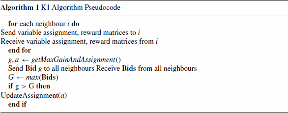
This paper focuses on the class of static estimation (SE) DCEE algorithms. The k=1 SE-optimistic algorithm, K1 from now on, allows a single agent to change variable(s) per neighbourhood. For instance, in Figure 1, if agent 2 changes its variable setting, agents 1 and 3 must remain fixed. Alternatively, if agent 1 changes its variable, agent 2 must remain fixed, but agent 3 could choose to change. The algorithm is optimistic in the sense that it estimates that it will receive the maximum reward on every constraint if it picks an unexplored configuration. This results in the behaviour that (1) every agent wishes to change configurations on every round, (2) the algorithm will always be exploring the environment (practically speaking, since our domain premise is that there are too many configurations to exhaustively cover during the given time frame), and (3) agents with the worst performance per neighbourhood will be allowed to explore. On every round, every agent will measure the reward between itself and all of its neighbours. It will then use Algorithm 1 to decide which agent (per neighbourhood) can choose a new assignment.

getMaxGainAndAssignment is a function that returns a variable assignment that maximises the difference between total expected reward across all binary constraints of the agent and its current reward. For the case of SE-optimistic algorithms, this will always be an unexplored position, because the agents are optimistic that such positions will have a very high potential reward. In this manner, for each neighbourhood, the agent with the worst performance across its binary constraints with neighbours will get to change its variable.

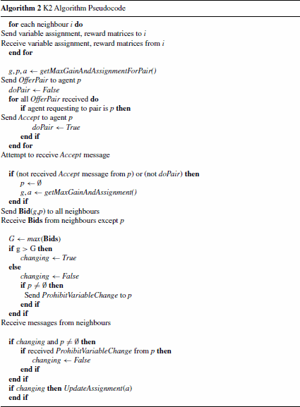
For the k=2 SE-optimistic algorithm, K2 from now on, each neighbourhood can allow up to two agents performing joint movement to change configurations (see Algorithm 2). Being an optimistic algorithm, it again assumes that any unexplored binary constraint will yield the maximum reward. Communication is more involved as the agents must first consider with whom they will likely form the pair with the most to gain (by assuming that the neighbour's neighbours would not change while evaluating the combined rewards). Each agent then sends an OfferPair message to their prospective partner, and those pairs that successfully match each other as the best in their vicinity will use that projected gain to compete with their respective neighbours’ bids. Should an agent not get a reply from the desired partner, though, it would evaluate the potential reward as would an agent in the k=1 scenario, and then bid using that value.

2.3 Reinforcement learning

The second approach we investigate in this paper is RL. RL (Sutton & Barto, 1998) is a machine learning paradigm that is aimed at learning (near-)optimal agent behaviour through interactions with an environment. This environment is typically formulated as a Markov decision process, which is a tuple , where S is the set of possible states of the environment, A the possible actions, T the dynamics of the environment (specified as state transition probabilities), and R the reward function (which attributes a utility to state transitions).

2.3.1 SARSA

One popular RL algorithm is SARSA (Rummery & Niranjan, 1994). It is a model-free method that estimates an action-value function, Q(s, a), measuring the expected return of taking action a in state s from experience. After each state transition, it updates its estimates according to where r_t represents the reward at time t for transitioning from state s_t to s_t+1, a_t is the action that caused that transition, and a_t+1 is the action that will be taken in state s_t+1. Under certain conditions (Singh, Jaakkola, Littman, & Szepesváari, 2000), these Q-value estimates converge to the true Q-values in the limit, and an optimal policy can be followed by taking the action with the largest Q-value in every state.

The problem considered in this paper is a multi-agent system, and thus the agents will be learning in the presence of other agents. This renders the problem non-stationary for learning agents that do not coordinate or take other's actions into account, and proofs guaranteeing convergence to the optimal policy of single-agent algorithms are invalidated. Still, independent learners often perform well, notwithstanding their lack of coordination (Busoniu, Babuska, & De Schutter, 2008), and therefore we will take this approach, keeping the algorithm as simple as possible.

2.3.2 Eligibility traces

Eligibility traces (Klopf, 1972) are records of past occurrences of state-action pairs. These traces can be used to speed up learning, by not only updating the Q-value of the current state–action pair, but also past state–action pairs, rewarding these inversely proportional to the time since they were experienced. A replacing eligibility trace (Singh & Sutton, 1996) e_t(s, a) for state s and action a is updated as follows:

It is set to 1 if (s, a) is the current state–action pair (s_t, a_t), and otherwise it is decayed by , with γ the standard RL discounting factor and λ the specific eligibility trace decay. This update is performed after every action, and thus traces decay over time. The trace is then included in the Q update rule

Instead of only updating Q(s_t, a_t), we update the Q-value of every state–action pair where the eligibility trace is non-zero. This effectively allows us to immediately propagate reward into the past, rewarding actions that lead to the current reward, significantly reducing the learning time. Otherwise, this reward propagates only by means of the part in the update-rule.

2.3.3 Tile coding

SARSA and other temporal difference methods are often implemented with look-up tables for the Q-values. However, when applying these algorithms to problems with large state and action spaces, or even continuous ones, memory requirements become an issue. Furthermore, an agent would need to visit every state–action pair multiple times to account for a potentially stochastic environment. Therefore, generalisation techniques are a necessity. Tile coding (Albus, 1981; Sutton & Barto, 1998) is one form of function approximation where the state-space is partitioned multiple times, i.e. into multiple tilings. Each tiling divides the space into a number of disjoint sets, or tiles. When a state is visited, it is mapped to exactly one tile in each tiling. Instead of directly estimating the Q-value of each state s and action a, the Q-function is decomposed into a sum of weights for each tile where n is the number of tiles and b_i is 1 or 0, depending on whether the tile is activated by state s and action a. Whenever a regular Q-value update would be executed, the weight of each activated tile is updated instead. Mapping states to different tilings and decomposing the Q-function into a linear combination of tilings allows the generalisation of experience between states that are similar. The more tiles two states share, the more generalisation will occur.

3. Experimental set-up

This section introduces the traffic simulator used in experiments, and a standard traffic benchmark algorithm. It also details the set-up used for DCEE and SARSA experiments.

3.1 The autonomous intersection management simulator

The autonomous intersection management (AIM) simulator is developed by the Learning Agents Research Group at the University of Texas at Austin. A microscopic traffic simulator, AIM supports a Manhattan topology of North–South and East–West multi-lane roads joined by a number of intersections. The primary vision of this project is to investigate a future where autonomous vehicles and intelligent traffic intersections would eliminate the need for traffic lights altogether. As part of their benchmark, however, the team has also implemented ordinary traffic lights into the system. For the purpose of our study, we made exclusive use of this benchmark feature as the backdrop against which traffic lights will be tested. Even though the traffic light system in AIM is implemented using the same message-passing foundation, the inherited efficiency in which vehicles navigate an intersection, accelerate, and decelerate, as well as subtle details including variable vehicle sizes, have convinced us that this is an attractive simulator for our purposes.

Our set-up involves single-lane two-way streets forming a 2×2 matrix of four intersections. Each road has two spawn points where new vehicles can enter the system. Each spawn point uses a Poisson process to determine the spawn time for the next vehicles; all spawn points share the same rate parameter, λ. Because each direction has one lane, a newly spawned vehicle will not pass other cars, nor does it perform U-turns. Upon creation, each vehicle is assigned a destination, uniformly chosen among the seven possible exit points of the system; the vehicle then follows the shortest path to reach its designated exit point, determined by applying A*.

3.2 Isolated actuated traffic signal benchmark

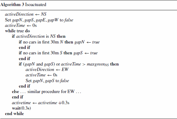
To have a reasonable upper bound on performance in our experiments, we implement a static benchmark algorithm (Minnesota Department Of Transportation, 2011; Pham, Tawfik, & Taylor,2013) that assumes knowledge of the distribution of traffic arriving at the intersection whose lights it is controlling. It follows the procedures described in Algorithm 3. The procedure is executed every 0.3 s, changing the direction of its lights (e.g. from North–South to East–West) only when the current direction (North-South) has been active for longer than maxgreen_NS, or when it has observed that there have been no cars within the first 30 m from both the N and S directions. The variable is crucial for the optimal working of this algorithm. To set maxgreen_NS and maxgreen_EW, one must first measure the proportion of cars taking left turns, right turns, and those going straight for each incoming direction at an intersection. Using this information, the maxgreen variables for these traffic distributions can be optimised using the software package PASSER^™ (Texas Transportation Institute, 2011). Note that this algorithm needs to know the traffic distribution in advance, and is non-adaptive; performance is not robust against changes in the traffic distribution.

3.3 DCEE experiments

In the set-up for the DCEE experiments, we make use of a special traffic light signal scheme that relies on the AIM simulator's definition of an ‘active phase’. Two parameters specify precisely such an active phase: the green offset and green duration in seconds (see Figure 2). For simplicity, our experiments will have the active phase length fixed at 60 s. We then associate each intersection with a DCEE agent, letting each agent control exactly one variable – its Signal Scheme Index. This index enumerates all possible traffic signal configurations, running from 0 to 65 (see Figure 3). Thus, index 0 maps to the tuple (0, 5), which is an active phase with no leading red, and 5 s of green time (followed by 2 s of yellow and 53 s of red). To translate the next index, we attempt to increase green time by a 5-s interval, while keeping the total active phase length. Should this not be possible, we instead increase the offset by 5 s, and reset green time to 5 s. This results in a triangular translation table, stopping at (55,5), for a total of 66 possible combinations. This discretisation of time is required as DCEE can only handle discrete actions. This is an inherent limitation of DCEE, although a fine-grained discretisation can be chosen as DCEE algorithms are specifically built to efficiently explore huge action spaces.

Figure 2. An example traffic light configuration that makes up an ‘active phase’ in the simulator.

Figure 3. The signal scheme index for each DCEE agent, and its corresponding (green_offset, green_time) value, defining an active phase of 60 s. Note that green_offset and green_time increase at 5-s intervals, a necessary discretisation.

Once the ‘active phase’ has been determined, the entire signal layout for each direction (North–South, East–West) will be specified as shown in Figure 4. Note that at any moment, only one direction is considered to be active (running the active phase signal scheme), and the other direction is inactive, running the complementary signal scheme.

Figure 4. The full signal scheme for an intersection, given a specific active phase. Time flows from left to right: the calculated active phase is active for North–South in the first 60 s, before switching to East–West in the next 60 s. The whole signal scheme repeats after 120 s total.

Agents evaluate the rewards of binary constraints with a neighbour by measuring the average travel time of the first 100 cars travelling on the stretch of road connecting the two agents. The total team reward at each round is then a weighted average of this average travel time. For our SE agents, we set the unexplored reward to be 0 s, an unattainable value for travel time. Since the DCEE algorithms are defined as maximisers, we negate the reward signal. Average travel time serves as a reasonable metric to optimise, as it correlates with other commonly used metrics that gauge traffic light performance, such as queue length and throughput, as we shall see in Section {4.2.1}. Thus, by letting the agents optimise for higher rewards in this context, we are letting the intersections work toward lower average travel time along the lanes between them, thus improving traffic light performance. After the agents have changed their signal schemes, we allocate a cool-down period of 600 s to allow the new signal schemes to have an impact on the traffic condition. Only after this cool-down period do the agents begin to evaluate rewards.

3.4 SARSA experiments

We apply SARSA with tile coding to the traffic light problem by giving control of each intersection to a SARSA agent. The SARSA set-up is as follows:

Every 2 s, the agents are presented with only two possible actions:

• (1) Do nothing or

• (2) change the green light to the other direction (e.g. from North–South to East–West).

Note that when changing the lights, a short period of yellow occurs, stopping traffic in all directions.

The state space is defined by three state variables:

• (1) The number of seconds since the most recent light change.

• (2) The number of seconds since the second-to-last light change.

• (3) The ratio between the queue lengths in both directions.

The first variable ensures that the agents will be able to learn a repeated schedule of fixed length. The inclusion of the second state variable allows the agents to learn asymmetrical schedules, which are useful when the traffic load is heavier in one direction than in the other. The third state variable allows the agent to adapt to the slight variations that occur in the general traffic pattern, by conditioning learning on the traffic load in each direction. Technically, the variable is a bit more than a simple ratio. We define to be the queue length in the green direction, and the queue length in the red direction. Now a simple ratio has an inherent asymmetry around 1, which would result in overgeneralisation of the states where the queue in the red direction is longer than the one in the green direction (for : ; for : ). Therefore, we encode the ratio as shown in Equation (1).

If we ensure that and are at least one, then var₃ will be 0 when queue lengths in both directions are exactly the same, and positive or negative when the queue is longer in the green or red direction, respectively. This ensures that, as opposed to using a simple ratio, this variable is symmetric around 0 and allows easy generalisation around 0 with linear tile coding. Furthermore, due to the logarithm, small differences in traffic are captured when the load is very similar in both directions, while the differences when the traffic is asymmetric are compressed. Tile size is 5 for the first two variables, and 1 for the third variable; 32 tilings are used over the three variables.

The reward that agents receive is the negation of the total accumulated waiting time for all cars approaching their intersection. Maximising this reward will reduce the average waiting time. Although the aim in the traffic problem is to optimise the whole traffic system, the reward agents receive is only local. Calculating the global reward by broadcasting the local rewards is costly, and furthermore, employing global reward introduces a credit assignment problem, which may hinder learning (Chang, Ho, & Kaelbling, 2004).

Note that including information on waiting times and queue lengths is not unrealistic. Modern road infrastructures include cameras and other sensors that are able to keep track of the traffic. Furthermore, the use of floating car data is increasing. This is a method used to calculate traffic speed based on signals from cellular and global positioning system devices in cars, providing real-time information on traffic.

The action-selection strategy used is ε-greedy: when an action must be selected in state s, the action with the highest estimated Q-value is selected with probability 1−ε, and with probability ε a different action is randomly selected. Furthermore, ε is decreased over time (, t the tth decision step, which occurs every 2 s), to increase exploitation of the acquired knowledge. The discounting factor γ, as well as the replacing eligibility traces’ decay λ, is set to 0.9.

3.5 Differences in set-up

As already remarked, the set-ups of the DCEE and RL algorithms have significant differences. First, their action spaces are different. Second, RL incorporates state which DCEE does not. Third, the RL approach involves decisions every 2 s, while the DCEE algorithms operate over much longer periods (at least 120 s). Direct comparisons between the approaches’ action selection will be inexact. However, it is not our purpose to evaluate these algorithms in that respect, but rather, for each approach we chose the most fitting set-up for the traffic problem, and illustrate their behaviour on this traffic problem. The DCEE set-up is built to quickly learn good policies matching the general traffic pattern, while the RL set-up is built to allow the SARSA agents to learn both the general traffic pattern, as well as the short-term variations in the pattern as it incorporates the current traffic distribution in its state.

4. Experiments

This section is split into two parts, with the first subsection discussing the effect of the traffic load on the DCEE and RL algorithms, and how they compare against the static benchmark algorithm. In the second section, we discuss the multi-objective nature of the traffic light control problem, and experimentally show how the asymptotic performance of the RL approach can be improved using alternative reward signals, including the combination of different reward signals.

4.1 Light versus heavy traffic

First we examine the impact of the level of traffic on algorithm performance. We run the simulator with a 2×2 grid for 90,000 s, in which we measure the agents’ performance in terms of the average delay per car and the total throughput. These metrics are the two most important measures used by engineers to compare control policies. While throughput indicates how many cars a system can process in a given time period, average delay gives an indication of how the system's performance affects individual cars’ travel time. Before the agents are allowed to learn, i.e. before the 90,000 s, we implemented a 7500 s warm-up period, in which the agents are forced to select random actions, to allow the system to fill with cars and reach an equilibrium. This warm-up period is not graphed in the figures.

We evaluate two settings with different traffic loads. The first experiment is parametrised to generate an average of 10 cars per minute, per entry link. In the second experiment, an average of 30 cars is generated each minute per entry location, a much heavier traffic level. For these traffic distributions, we optimised the variables in the isoactuated benchmark. For the heavy traffic, we set it to and for agents 1 and 3, and the reverse for agents 2 and 4.¹ For light traffic, for all agents.

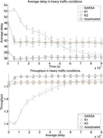
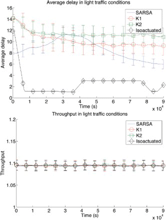
Figure 5 shows the performance of SARSA, K1 and K2, and the isoactuated benchmark on the light traffic setting. Experiments are averaged over 100 runs for statistical significance, and error bars show one standard deviation. Each datapoint is a running average over 100 min. The first notable observation we make is that with so little traffic, it is not possible to improve the throughput of cars. On the other hand, the algorithms can clearly improve the average delay. Notably, SARSA performs much better than K1 and K2, as it is not limited to the (too long for light traffic) 60 s schedules, but incorporates the actual traffic situation in its state, and adapts to that. K2 performs worse than K1, even though it involves more coordination between the agents. This apparent discrepancy is due to a phenomenon coined the team uncertainty penalty (Taylor et al., 2011), in which agents with few neighbours actually achieve higher performance with lower levels of coordination (e.g. K1), while agents with many neighbours can achieve higher performance with higher levels of coordination (e.g. K2). Finally, we note that the static benchmark algorithm performs significantly better than the adaptive approaches in terms of average delay, as it knows the actual traffic distribution in advance.

Figure 5. Average delay and throughput for a light traffic level (10 cars spawned per minute at each entrance). Error bars show one standard deviation.

Let us now consider the heavier traffic setting experiment, shown in Figure 6. Both throughput and average delay can be greatly improved upon in this setting. SARSA starts with very poor performance for both measures compared to DCEE algorithms, due to the inherent bias in the action selection given the definition of the DCEE action space. However, SARSA is able to learn a great deal (approaching the performance of the isoactuated benchmark), and in the end it outperforms both DCEE algorithms as these are stateless and cannot adapt to the local, ephemeral fluctuations in the traffic pattern. The power of the DCEE framework is demonstrated by the fast improvement of K1 and K2 as measured by average delay. Between two adjacent changes in signal schemes, the agents spend 600 s for the cool-down period, and about 600 s for collecting data to measure average travel times. Thus, both K1 and K2 are able to significantly optimise the traffic flow of the system in only eight decision steps (around the 10,000 s mark), with possible schedule combinations to choose from. Furthermore, throughput is only slightly improved as it already is at a near-optimal level for any possible schedule. SARSA needs much longer to achieve that level of performance, because it must learn to extend the length of its green periods, while the DCEE algorithms are limited to 60 s schedules and automatically have long periods of green. From this we can conclude that to optimise throughput in a traffic system, a major factor is to have green periods that are long enough. For delay, performance also depends on having long enough green periods, but even more on balancing between the different directions (it is possible to maximise throughput by only changing the lights when the queue in the current green direction is cleared, while this is not an optimal policy for delay). Lastly, it is interesting to note that in both experiments, SARSA first decreases its performance as compared to random, before it is able to improve again.

Figure 6. Average delay and throughput for a heavy traffic level (30 cars spawned per minute at each entrance). Error bars show one standard deviation.

4.2 Alternative reward signals

In this section we evaluate several alternative reward signals for SARSA.² In the first subsection, we give a brief analysis of the multi-objective nature of the traffic optimisation problem, and go on to show how the objectives can be combined to improve performance. In the second subsection, we look at delay squared, a reward signal that heavily punishes large delays, while neglecting small differences in short delays.

4.2.1 Traffic optimisation: a multi-objective problem

Traffic optimisation is inherently a multi-objective problem. In this work, we measure an algorithm's performance by both looking at average delay and throughput, i.e. the two objectives we want to optimise. In the previous section, we have only considered one of the two objectives as a feedback signal for our learning agents, yet they were able to improve performance on both metrics. This leads us to assume that these two objectives are correlated. To confirm this hypothesis, we show the observed measurements of both metrics during a single RL run with delay as reward signal in Figure 7(a). A brief visual inspection indicates the objectives are correlated, and calculating the Pearson product–moment correlation coefficient yields a ρ-value of −0.7952. This shows that the objectives are highly correlated; the ρ-value is negative since delay must be minimised, while throughput must be maximised. Note that the optimisation process can also be observed in the figure, as measurements early in the experiment (blue) are dominated by the measurements near the end of the experiment (red).

Figure 7. The reward samples observed during a single run with a heavy traffic level and either delay (a) or throughput (b) as a reward signal. Colour indicates the timing of the sample, with blue early in the run, and red at the end of the run. The objectives (minimising delay on x-axis and maximising throughput on y-axis) are observed to be correlated.

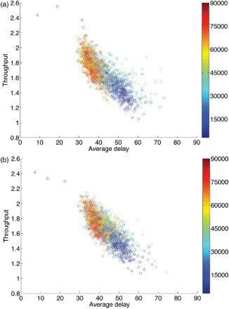
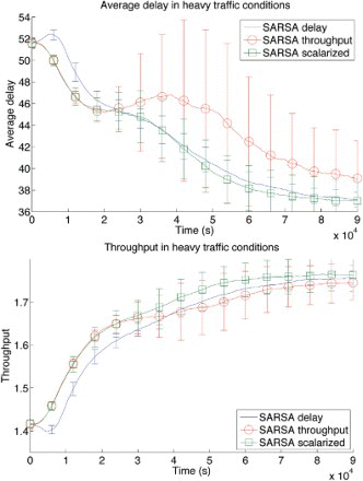
Replacing delay with throughput³ as a reward signal yields similar correlated measurements as shown in Figure 7(b), and a Pearson product–moment correlation coefficient of −0.7821. In Figures 8 and 9, we show the performance for each objective when using throughput as a reward signal. Note that we no longer plot the throughput measurements for the light traffic setting, as none of our experiments show improvements for throughput in that setting. We observe that the throughput signal is better suited for optimisation than delay in light traffic conditions, while the reverse is true in heavy traffic conditions.

Figure 8. Average delay for a light traffic level (10 cars spawned per minute at each entrance). Comparison of two single-objective approaches and linear scalarisation. Error bars show one standard deviation.

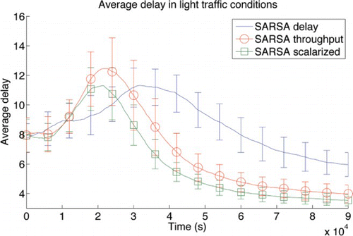
Figure 9. Average delay and throughput for a heavy traffic level (30 cars spawned per minute at each entrance). Comparison of two single-objective approaches and linear scalarisation. Error bars show one standard deviation.

Ideally, we would combine the objectives in such a way that we can have the best of both in any situation. Therefore, we replace the single-objective reward signal by a scalarised signal (VanMoffaert, Drugan, & Nowé, 2013), combining both objectives using a weighted sum Figures 8 and 9 show the results using SARSA learning with this scalarised reward signal with finely tuned weights. Weight tuning was initially guided by the differences in scaling of both objectives (delay approximately ∈[0, 50], throughput approximately ∈[0, 2]). The first weights tested were for throughput and delay, respectively: and . Subsequent rounds of tuning showed that w_d should be even smaller, and the final selected weights are: w_t=0.991 and w_d=0.009. We see that using this linear scalarisation, we can actually get the best of both objectives, and more. In the setting with a light traffic level, this scalarisation helps converge faster to a better asymptotic level of performance than both single objective signals. Looking at delay in the setting with a heavy traffic level, learning with the scalarised signal first follows the same curve as using only throughput, and when single-objective throughput's performance degrades, the scalarised learning curve starts following the delay curve, basically taking the best parts of both curves. For the throughput metric, scalarised SARSA again improves asymptotic performance.

The reason why we can achieve such good results using a simple weighted sum is as follows. By tuning the weights, we are basically aligning the objectives, so that similar differences in performance are reflected as reward differences of similar magnitude (a form of normalisation). Having aligned the objectives well enough, we are basically reducing noise by combining two signals that point roughly in the same direction (since they are highly correlated). The scalarised signal will therefore be more reliable than either single objective alone, and learning proceeds faster.

4.2.2 Delay squared

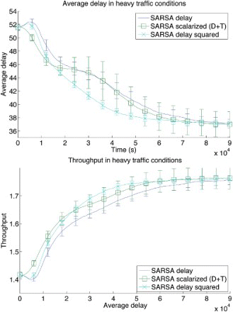
Another possible reward signal is delay-squared, i.e. the delay signal raised to the power of 2. This reward formulation allows us to punish large delays much more than small delays, making the agents more sensitive to variations in very large delays. Figure 10 shows the comparison among using delay, delay-squared, scalarisations of delay and throughput, and scalarisations of delay-squared and throughput (using the same weights as before) in light traffic. Throughput is again not plotted because no improvements are observed with any algorithm. For the heavy traffic (Figure 11), the latter scalarisation is not shown as it performs the same as delay-squared alone. This makes sense, as we have already shown that throughput is not the best reward signal in that setting. Additionally, we can see that delay-squared results in even faster learning in both traffic settings, although with worse asymptotic performance in the light traffic setting. Combining it with throughput resolves this problem, at the cost of slower initial learning. Notice also the small standard deviations, indicating that using delay-squared as a reward signal results in more reliable learning.

Figure 10. Average delay for a light traffic level (10 cars spawned per minute at each entrance). Comparison of delay, scalarised (delay and throughput), delay-squared and a different scalarised (delay squared and throughput) reward signal. Error bars show one standard deviation.

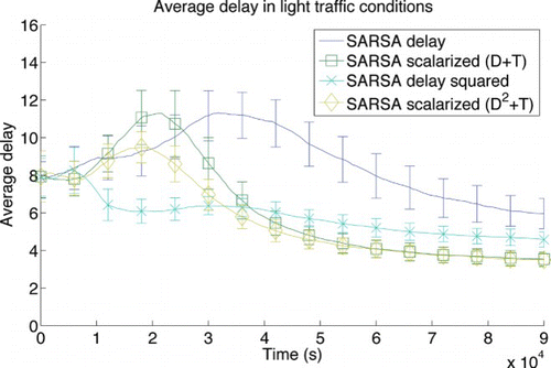
Figure 11. Average delay and throughput for a heavy traffic level (30 cars spawned per minute at each entrance). Comparison of delay, scalarised (delay and throughput) and delay-squared reward signals. Scalarised with delay-squared and throughput yields the same performance as delay-squared alone. Error bars show one standard deviation.

5. Conclusions and future work

In this study we analysed the traffic light control problem, looking at the behaviour of two classes of learning algorithms in the context of different traffic loads, and the multi-objective nature of the problem itself. We observed that with light traffic loads, only the delay metric can be significantly optimised, as throughput is near-optimal for most reasonable schedules. Furthermore, it is clear that incorporating the current state of the traffic in the decision making process allows for much finer control and response to fluctuations in the general traffic pattern. Also, applying algorithms from the DCEE framework, our previous results concerning the team uncertainty penalty are confirmed in this setting (Taylor et al., 2011), showing again that more coordination among agents is not necessarily beneficial.

In the second part of the experimental study, we considered the multi-objective nature of the traffic problem. We show how the two metrics that are most commonly used to measure performance, i.e. delay and throughput, are correlated. This explains why optimising based on a feedback signal of measurements of either metric alone yields improved performance on both metrics. When combining these signals in a naive way using a weighted sum, we showed that significant improvements in performance can be achieved, the sum being greater than the parts. Furthermore, using delay-squared, alone or combined with throughput, yields further improvements in performance.

One significant disadvantage attached to the scalarisation approach is that in order to achieve good performance, the weights need to be tuned very carefully. This weight tuning can be expensive in settings such as this, requiring many hours or days of simulation to find good parameters. Future work includes formulating an approach that can take optimal advantage of these correlated weights, without requiring parameters to be set, and importantly, without depending on the scaling of the objectives, which is one reason why weight tuning is necessary in the first place.

Acknowledgements

We thank the reviewers for their helpful suggestions and comments. Tim Brys is funded by a PhD grant of the Research Foundation-Flanders (FWO), and performed a research visit to Prof. Matthew E. Taylor at Lafayette College, funded by a Short Stay Abroad grant also from the FWO. This work was supported in part by NSF IIS-1149917.

Notes

1. Agents are ordered in a 2×2 grid, with numbering starting top-left and ending bottom-right.

2. We continue only with RL as it produced better asymptotic performance in the previous experiments (i.e. Figures 5 and 6).

3. Local throughput is measured by counting the number of cars that cross the intersection, and dividing by the time period measured. This time period is the time between two actions, i.e. 2 s for a ‘stay’ action, and 4 s for a change action (accounting for the 2 s yellow light). We divide by the time period to account for actions of different duration.

References

- Albus, J. (1981). Brains, behavior and robotics. New York, NY: McGraw-Hill, Inc.
- Bazzan, A. L. C., & Klügl, F. (2013). A review on agent-based technology for traffic and transportation. The Knowledge Engineering Review. FirstView. 10.1017/S0269888913000118. Retrieved from http://journals.cambridge.org/action/displayAbstract?fromPage=online&aid=8907641.
- Busoniu, L., Babuska, R., & De Schutter, B. (2008). A comprehensive survey of multiagent reinforcement learning. IEEE Transactions on Systems, Man, and Cybernetics, Part C: Applications and Reviews, 38(2), 156–172. doi: 10.1109/TSMCC.2007.913919
- Chang, Y.-H., Ho, T., & Kaelbling, L. P. (2004). All learning is local: Multi-agent learning in global reward games. In S. Thrun, L. Saul, & B. Schoelkopf (Eds.), Advances in neural information processing systems 16. Cambridge, MA: MIT Press.
- Dresner, K., & Stone, P. (2008). A multiagent approach to autonomous intersection management. Journal of Artificial Intelligence Research, 31, 591–656.
- El-Tantawy, S., Abdulhai, B., & Abdelgawad, H. (2013). Multiagent reinforcement learning for integrated network of adaptive traffic signal controllers (MARLIN-ATSC): Methodology and large-scale application on downtown Toronto. IEEE Transactions on Early Access Intelligent Transportation Systems, 14(3), 1140–1150. doi: 10.1109/TITS.2013.2255286
- Junges, R., & Bazzan, A. (2008). Evaluating the performance of dcop algorithms in a real world, dynamic problem. Proceedings of the 7th international joint conference on autonomous agents and multiagent systems, International Foundation for Autonomous Agents and Multiagent Systems, Richland, SC, pp. 599–606.
- Klopf, A. H. (1972). Brain function and adaptive systems: A heterostatic theory (Technical Report AFCRL-72-0164). Bedford, MA: Air Force Cambridge Research Laboratories.
- Kuyer, L., Whiteson, S., Bakker, B., & Vlassis, N. (2008). Multiagent reinforcement learning for urban traffic control using coordination graphs. Machine Learning and Knowledge Discovery in Databases, 5211, 656–671. doi: 10.1007/978-3-540-87479-9_61
- Liu, Z. (2007). A survey of intelligence methods in urban traffic signal control. IJCSNS International Journal of Computer Science and Network Security, 7(7), 105–112.
- Minnesota Department of Transportation. (2011). Traffic signal timing and coordination manual. Minnesota Department of Transportation.
- Mirchandani, P., & Wang, F.-Y. (2005). Rhodes to intelligent transportation systems. IEEE Intelligent Systems, 20(1), 10–15. doi: 10.1109/MIS.2005.15
- National Transportation Operations Coalition. (2012). National traffic signal report card, executive summary. Retrieved from http://www.ite.org/reportcard/ExecSummary.pdf.
- Pham, T. T., Tawfik, A., & Taylor, M. E. (2013). A simple, naive agent-based model for the optimization of a system of traffic lights: Insights from an exploratory experiment. Proceedings of the conference on agent-based modeling in transportation planning and operations, Blacksburg, VA.
- Robertson, D., & Bretherton, R. (1991). Optimizing networks of traffic signals in real time-the scoot method. IEEE Transactions on Vehicular Technology, 40(1), 11–15. doi: 10.1109/25.69966
- Rummery, G., & Niranjan, M. (1994). On-line Q-learning using connectionist systems. Cambridge: Department of Engineering, University of Cambridge.
- Shoufeng, M., Ying, L., & Bao, L. (2002). Agent-based learning control method for urban traffic signal of single intersection. Journal of Systems Engineering, 17(6), 526–530.
- Singh, S. P., Jaakkola, T., Littman, M. L., & Szepesvári, C. (2000). Convergence results for single-step on-policy reinforcement-learning algorithms. Machine Learning, 38(3), 287–308. doi: 10.1023/A:1007678930559
- Singh, S. P., & Sutton, R. S. (1996). Reinforcement learning with replacing eligibility traces. Machine Learning, 22(1–3), 123–158. doi: 10.1007/BF00114726
- Sutton, R., & Barto, A. (1998). Reinforcement learning: An introduction. Cambridge: Cambridge University Press.
- Taylor, M. E., Jain, M., Tandon, P., Yokoo, M., & Tambe, M. (2011). Distributed on-line multi-agent optimization under uncertainty: Balancing exploration and exploitation. Advances in Complex Systems (ACS), 14(03), 471–528. doi: 10.1142/S0219525911003104
- Texas Transportation Institute. (2011). Passer (tm) v-09. Retrieved from http://ttisoftware.tamu.edu/
- Thorpe, T., & Andersson, C. (1997). Vehicle traffic light control using SARSA (Master's thesis). Department of Computer Science, Colorado State University, Fort Collins.
- Van Moffaert, K., Drugan, M. M., & Nowé, A. (2013). Scalarized multi-objective reinforcement learning: Novel design techniques. Proceedings of the IEEE symposium on adaptive dynamic programming and reinforcement learning, Singapore, pp. 94–103.