Anticipation by multi-modal association through an artificial mental imagery process

Abstract

Mental imagery has become a central issue in research laboratories seeking to emulate basic cognitive abilities in artificial agents. In this work, we propose a computational model to produce an anticipatory behaviour by means of a multi-modal off-line hebbian association. Unlike the current state of the art, we propose to apply hebbian learning during an internal sensorimotor simulation, emulating a process of mental imagery. We associate visual and tactile stimuli re-enacted by a long-term predictive simulation chain motivated by covert actions. As a result, we obtain a neural network which provides a robot with a mechanism to produce a visually conditioned obstacle avoidance behaviour. We developed our system in a physical Pioneer 3-DX robot and realised two experiments. In the first experiment we test our model on one individual navigating in two different mazes. In the second experiment we assess the robustness of the model by testing in a single environment five individuals trained under different conditions. We believe that our work offers an underpinning mechanism in cognitive robotics for the study of motor control strategies based on internal simulations. These strategies can be seen analogous to the mental imagery process known in humans, opening thus interesting pathways to the construction of upper-level grounded cognitive abilities.

Keywords:

• mental imagery
• cognitive robotics
• anticipation
• multi-modal association

1. Introduction

Over the last two decades a new school of thought has taken shape in artificial intelligence laboratories. As in other areas, the ideas of grounded cognition (Barsalou, 2008) have taken central stage. In this framework, sensorimotor associations, occurring during the active interaction of an agent with its environment, are central for the development of cognition. Current research in cognitive developmental robotics (Asada et al., 2009) aims at developing basic cognitive skills in robots drawing inspiration from knowledge, studies and experiments on human development (see Tikhanoff et al., 2011 for a thorough review).

A long history of research in cognitive sciences converges in that anticipation is an ability of the utmost importance for animals and humans (Butz et al., 2002). Even though, for the advocates of motor-based theories of cognition, the underlying mechanisms of anticipation remain an open question (Pezzulo, 2008); i.e. those non-representational mechanisms underlying a time-scaled organisation of action accounting for long-term behaviour.

The hypothesis we aim at validating experimentally in this work is that an anticipatory behaviour emerges from a multi-modal association process, taking place during the internal simulation of sensorimotor cycles. Internal simulations, regarded as recreations of perceptual, motor and introspective states, are thought to be in play in a wide variety of mental phenomena and are considered to lie at the heart of the off-line characteristics of cognition (Wilson, 2002). In particular, we are concerned with the internal simulation phenomenon known as mental imagery (Barsalou, 2008; Kosslyn, 1994), considered by many researchers as a basic cognitive capability and supported by neural evidence (e.g. see Kosslyn et al., 2006).

Mental imagery is an internal process that re-enacts a physical experience in the absence of actual appropriate stimulus; its primary function is the generation of specific predictions based upon the past experience (Moulton & Kosslyn, 2009). In recent times, the formal investigation of imagery in robotics has gained momentum (e.g. Di Nuovo et al., 2013; Frank et al., 2012; Kaiser et al., 2010; Schenck et al., 2012). The aim is ‘to understand the role of mental imagery and its mechanisms in human cognition and how it can be used to enhance motor control in autonomous robots’ (Di Nuovo et al., 2012, p. 1).

Research in imagery has been undertaken for long in most of the cognitive sciences. Among the findings that have been reported in the literature, our work considers three functional properties of mental imagery.

First, there are structural constraints in the architecture supporting this process, for in humans, the same neural machinery used to imagine the future is used to remember the past (Schacter et al., 2007). This concern is relevant from the perspective of the computational mechanism underpinning internal simulations.

Second, Driskell et al. (1994) observed that mental practice, defined as a cognitive rehearsal of a task prior to its execution, increases performance in athletes. This could be viewed as a reinforcement scheme of sensorimotor coordination through a reiterative off-line process, an aspect we incorporate in our model.¹

Last but not least, Dadds et al. (1997) report experiments with humans that account for classical conditioning through imagery. Their evidence suggests that off-line visual representations can create a new link between a conditioning stimulus and an unconditioned reflex in some forms of conditioning in humans. This conditioning feature of imagery is the third aspect we investigate in our work.

We propose a new motor control scheme based on a visual conditioned response synthesised by means of an off-line association of multi-modal stimuli. This occurs during an internally simulated chain of predictions, thus emulating a mental imagery process. To the best of our knowledge, this control scheme, obtained from the hebbian association of a covert chain of sensorimotor predictions, has not been reported in the literature. We investigate how this off-line association process accounts for an anticipatory response in obstacle avoidance behaviour, allowing the agent to cope with future undesirable situations with no explicit representation of the undesired stimulus. We implemented the system in a physical robot and report experiments for navigation tasks in static environments.

The structure of the paper is as follows. Section 2 describes the lower level of our architecture based on a forward model predicting visual and tactile sensory patterns. In Section 3 we introduce our computational model and the off-line association process leading to the anticipatory functionality. We then show and discuss the experimental results in Section 4 and conclude the paper in Section 5.

2. Sensorimotor predictions and internal simulations

In this section we introduce the predictive model we used and the internal simulation process. We also discuss functional properties of the system that are relevant to set down the basis of the present work.

2.1. Forward model for visual and tactile predictions

In the quest of a basic simulation mechanism, forward and inverse models have been proposed (e.g. Grush, 2004; Miall & Wolpert, 1996; Wolpert et al., 2001). These pairings have been studied and implemented for control and planning purposes in different applications.²

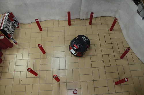
We have reported in Escobar et al. (2012) an artificial agent (shown in Figure 1) capable of predicting the position of obstacles in its environment, by re-enacting visuo-motor cycles to detect collisions from visual data. To this end, we used a forward model to learn sensorimotor associations from the visual, tactile and motor modalities. These associations allowed the agent to predict distances to objects in terms of its own body characteristics; i.e. we are not aiming at computing a distance in metric units. We recall now the main features of this model.

Figure 1. Artificial agent: Robot Pioneer 3-DX with an array of 8 sonars and a stereo camera at front.

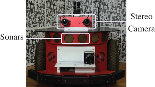
The visual modality is a maximum disparity vector (MDV) extracted from the disparity map (DM). We use the DM as a visual sensor reading that provides an implicit measure of distance to objects and a reduced input space.

From the difference between right and left images coming from the stereo camera the DM is computed, out of which a 228×6 region of interest (ROI) is extracted (see Figure 2). The upper limit of the ROI is located at line 152 of the image, which in a scene without obstacles is located at 2.15 m from the robot. This is the maximum distance for which a disparity value can be calculated. In the horizontal axis 228 pixels are taken, as they constitute the effective processed area of the image given the size of the masks used for computing the disparity. The MDV is formed by taking the maximum disparity value in each column of the ROI and represents the closest obstacles in the last 57.3° of the field of view.

Figure 2. Visual processing to obtain the MDV. For a detailed explanation of the system refer to Escobar et al. (2012).

The second modality is tactile and is formed by a bumper vector (BV) of 228 values to keep correspondence with the size of the MDV for associative purposes. This vector represents a single binary bumper, activated as a whole when there is a collision, irrespective of where this occurred in the body of the agent. The aim is to relate a collision state with the visual disparity information. The bumper states are constituted by the readings of the two frontal sonar sensors after being trimmed to a threshold value. All BV values are set to one when a collision is detected by either frontal sensor, and to zero otherwise.

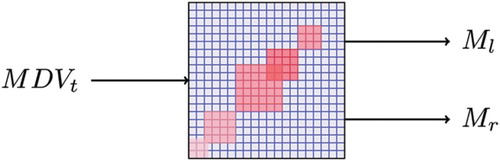
The implemented forward model is shown schematically in Figure 3. It takes as input the 228 values of the MDV vector and a motor command at time t: and M_t, respectively. The output is constituted by and , the visual and tactile modalities at time t+1, respectively. The model is coded using local predictors imitating the biological structure of visual sensors and thus reducing the numerical complexity of the task. Each of the local predictors takes as input a 14-value window from the MDV vector at time t, and predicts four central values of each output vector at time t+1. This results in 57 multilayer perceptron networks which are trained using resilient back propagation (Riedmiller & Braun, 1993).

Figure 3. Schematic view of the implemented forward model showing the input at time t and predicted output at time t+1. The visual sensory input together with the motor command triggers a prediction of visual and tactile sensory situations.

For training purposes, we used a constant motor command. However, it is important to stress that the predicted sensory situation at time t+1 is a consequence of the particular action executed at time t. Hence, the motor command is coded in the structure of sensory data: if the control changes output data would change accordingly. The networks were trained with data collected while the agent performed forward motions in an environment surrounded by obstacles. To account for the embodied character of our approach, the motion is quantified in robot steps corresponding to approximately 15 cm of displacement in the frontal direction. We used standard procedures for training and testing, using 2259 patterns coming from distinct environment settings (80% of which were used for the training phase).

2.2. Embodied internal simulation process

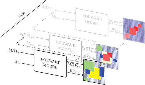
The internal simulation process is made of what we call long-term prediction (LTP). To build an LTP, we use the output of the forward model as input again and repeat this process for a defined number of steps. Figure 4 shows a number of actual MDVs compared with predictions coming from an LTP for a typical run of five steps. The first column shows the actual MDV at each step, where the initial state is the top row of the image. Dark regions indicate the absence of obstacles, while grey to bright regions report obstacles that are increasingly closer. The next column on the right shows the resulting predictions when an LTP is launched at the same initial state for an equal number of steps.

Figure 4. LTP of the MDV for five steps, ending in a collision on the right-hand side of the robot. (a) Evolution of the actual MDV vector (a row of 228 values) each time the robot moves ahead (5 steps shown). The brightness of the regions indicates increasing proximity of an obstacle, therefore two obstacles on the right-hand side of the robot get closer as the agent moves. (b) 5-step prediction of the same vector starting at the same initial time.

This LTP represents an internal simulation of what would happen in case the agent executed a number of motor commands; this process is akin to the off-line character of embodied cognition.

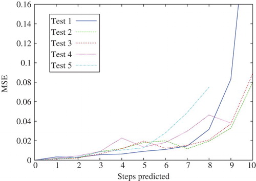
To evaluate the accuracy of the simulation process, we let the agent perform an LTP and then computed the mean-squared error (MSE) over the MDVs on five different scenarios. This is depicted in Figure 5, where the results of each scenario are labelled as Tests 1–5.

Figure 5. MSE over the 228 values of the MDV during an LTP of 10 steps.

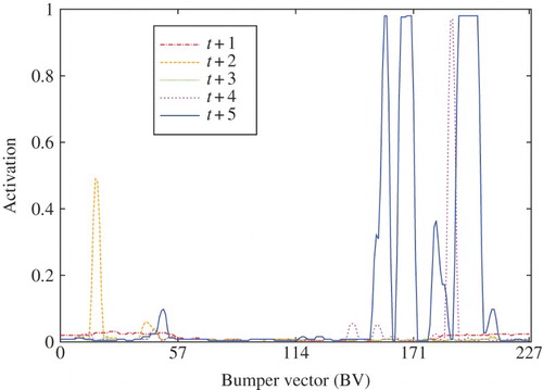
It is important to highlight the characteristics of the BV activation values. In Figure 6 predicted tactile values are plotted for five steps of an LTP. For training purposes, BV values were set to zero or one. However, during testing we observed that predicted values are continuous in the range [0, 1]. Moreover, the activated values correspond with the position of obstacles in the field of view of the agent; i.e. the activated neurons coding bumper states topologically correspond to the spatial distribution of obstacles in the MDV space (see Figure 4).

Figure 6. Five cycles of LTP for neurons coding bumper states.

In order to prove that the BV activation was neither a mere artefact of network connections nor a direct correlation of visual data, several control experiments were realised.

First, the same system was trained with a BV filled with only zeros. The resulting system showed no BV activation in the presence of obstacles in the MDV space. Second, the next outward pair of sonar sensors was used to obtain BV data for training. In this case, the BV activation continues to be correlated with the distribution of obstacles in the environment. The difference is now that the activation changes according to the new position of the sensors. During an LTP, obstacles ahead of the robot produce an activation one or two steps later than when using the frontal sensors. When obstacles are at the sides of the robot the opposite is true, obstacles are detected a step or two earlier than when frontal sensors were used. In other words, the tactile prediction exhibited by the BV activation accounts for the structure of the environment, and reflects the fact that activation is correlated with the physical distribution of the actual bumpers used during training.

This embodied character of the predictive process is instrumental in the association of both modalities as will be explained in the next section.

3. Learning by means of an artificial imagery process

3.1. Off-line learning process

The forward model provides means to predict visual situations; it allows the robot to know the consequences, in terms of a tactile modality, of moving overtly in one single direction. Yet, the robot does not make use of its motor capabilities to safely avoid obstacles. The agent lacks the notion of a collision emerging from the association of visual information, bumper states and motor commands.

We propose to provide the agent with means to imagine future situations, based on the current scenario, and to associate the corresponding off-line multi-modal flows, so as to develop an anticipatory motor control strategy to avoid obstacles. The obtained behaviour would not be a mere reaction to a bumper (tactile) activation, but the result of the visual anticipation of future occurrence of that activation.

To synthesise our grounded controller, we suggest an off-line learning technique, based on the association of two sensory modalities during LTP. To achieve this, we use a neural network configuration where the synaptic weights are subject to a hebbian learning process (Hebb, 1949).

In contrast to the current work found in the literature, we apply hebbian learning to system connections during internal simulations of predicted sensorimotor flows. The system can be seen as performing an off-line association process, through the simulation of sensorimotor cycles. This process relates motor and different sorts of sensory modalities, resembling the introspective feature of grounded and embedded cognition (Barsalou, 2008).

To the best of our knowledge this is a novel form of exploiting sensory predictions in order to create an anticipatory sensorimotor mechanism.

3.2. Computational model

3.2.1. Model concept

The original motivation of Donald Hebb was to find reasons behind different behaviours in subjects. He discovered that adjacent neurons that were active at the same time tended to reinforce their mutual connection: ‘what fires together wires together’ in cells of the central nervous system.

In a mathematical form, this rule can be expressed by

where w_ij represents the strength of the connection between neuron i and neuron j, and x and y are their respective outputs. Equation (1) represents the update of the synaptic weights and Equation (2) the magnitude of this change.

This learning process accounts for correlated neuron activity, based on the fact that synaptic weights are modified only when pre-synaptic and post-synaptic signals are active at the same time. In addition, it is an iterative mechanism as every time the neural network is active its synaptic weights are updated.³

In our case, we profit from the simultaneous firing of visual and tactile modalities provided by the forward model so as to emulate the pre-synaptic and post-synaptic signals.

A well-known implementation of Hebb's rule in robotics is known as DAC – distributed adaptive control (Verschure et al., 1992). Inspired by classical conditioning (Pavlov & Anrep, 2003), the goal of this architecture is to provide an autonomous agent with the ability to move safely in an environment amongst obstacles. The model assumes that an organism has a basic set of unconditioned stimuli (US), which automatically triggers an unconditioned response (UR). This US–UR reflex is genetically predefined to allow survival. A conditioned stimulus (CS) could then, by means of a learning process, be linked to the US and potentially trigger the UR. In other words, this process creates a new connection CS-UR, based on the relationship US–UR.

In the system we propose (see Figure 7(a)), the US is represented by bumper values, as these can be directly related to a collision and therefore drive the motor response (UR). By its very nature, the MDV does not contain any tactile information, thus the hebbian association of visual and tactile modalities can be used to mediate a CS. This CS would then drive an obstacle avoidance response (CR), in the presence of an obstacle in the current visual field. The computational architecture can be divided into two phases: a training phase and an execution phase (see Figure 7(b)).

Figure 7. Conceptualisation of the intended association mechanism. (a) Intended association by means of hebbian learning. (b) Computational architecture divided into two phases: (b.1) Off-line training phase. Motor commands are covertly executed. The forward model described in Section 2 enacts sensorimotor cycles producing visual and tactile predictions MDV_t+1 and BV_t+1. These in turn are fed to the association network where the hebbian learning process occurs. No motor commands are sent to the effectors as this process runs off-line (internal simulation); (b.2) Testing phase. The current visual situation MDV_t is fed into the association network which becomes a controlling network. Actual left (M_l) and right (M_r) motor commands are overtly executed.

Our assumptions are as follows:

1. The implemented forward model is capable of performing a reliable LTP of sensory states for both the MDV (CS) and the BV (US).

2. By hebbian learning, an association between MDV (CS) and motor output (UR) can be constructed in terms of a matrix of weights; this association is modulated by the BV (US).

3. The result of this association should code for desired behaviour, namely obstacle avoidance.

We describe now the learning process in detail. In Figure 8, we represent the execution of an LTP by re-enacting a number of intended forward movements (simulation chain). Visual and tactile sensory predictions of the trained forward model enter an association network where the hebbian learning process occurs.

Figure 8. Off-line association process. During the learning phase, the output of the forward model is fed again as input in what we call a process of long-term prediction (LTP). For every cycle in LTP, the weights in the association network (coloured squares) are modified through hebbian learning.

Starting at time t, actual and M_t values are used to predict and , which modulate the hebbian network. Next, the output is sent as the input to the next link of the simulation chain to obtain the next sensory situation and . This process is re-enacted to complete an LTP for a number of steps. During training, three to five steps of LTP are possible before the forward model reports a collision.⁴

Once trained, this network couples the current MDV or CS with the necessary motor command to deal with obstacles in the environment. Hence, motor commands are overtly executed, based only on visual information provided by the MDV as shown in Figure 9.

Figure 9. Once trained, the system becomes a controlling network with only visual input. M_l and M_r are left and right motor controls, respectively.

3.2.2. Model formalisation

The association network (Figure 10) consists of a 3-layer architecture. In order to further reduce the dimensionality of input space, we computed new vectors for both MDV and BV: we call D the new disparity vector and B the new BV. Each element of either new vector is the average value of four consecutive elements of the original vector (recall that both MDV and BV vectors have 228 elements). Hence, D and B are vectors of size 57.

Figure 10. Association network topology for mathematical formalisation. See the text for explanation.

Accordingly, each of the first two layers of the architecture contains 57 neurons. Each neuron of layer I receives an element of D, and is fully connected to layer II. Layer III has two neurons controlling left and right motors. The first 29 neurons of layer II are connected to the first neuron of layer III and the last 29 neurons to the second neuron (see Figure 10).

Let X be the output of layer I, produced by a linear function activation delivering the same received D. Let W be the 57×57 square matrix of all synaptic weights connecting layer I to layer II. We call U the input to layer II corresponding to a 1×57 vector that represents the weighted sum of the product X· W:

Let Y be the 1 × 57 activation vector of layer II which is a function of U. Each value y_i of Y is calculated through a sigmoid function and is given by

where the offset value δ is determined experimentally in order to achieve a minimum activation threshold in layer II during the learning process.

During the learning phase, the hebbian modulation is performed under the influence of B. The synaptic weights update follows the hebbian rule:

where is the synaptic weight change; η is the learning rate; B_d is a 57×57 diagonal matrix, where each element of the diagonal corresponds to each element of B; ε(t) is the forgetting factor varying in time; and is the average of the output of all neurons in layer II.

We let the outputs of layer II have an equal contribution to neurons in layer III, therefore connections from layer II to layer III have constant weights set to 1; the activation Z corresponds to the output of the two neurons in layer III: where z₁ and z₂ correspond to the activation of left and right motors, respectively.

4. Experimental results and discussion

The system was assessed by means of two experiments. In the first experiment one individual is trained and then tested in two different mazes. In the second experiment five individuals are trained with slight variations on the positions of obstacles in the learning arena. Performance of these individuals is then assessed in a navigation behaviour test.

In both experiments, the training aims at obtaining a modulation of the associative network apt to the task at hand.

4.1. One individual, two mazes

4.1.1. Training phase

The experimental setting during the learning phase is shown in Figure 11. Placed in the centre of the arena, the agent performs LTP until a crash with an obstacle is detected. Then the robot turns randomly (motor babbling), facing a different set of obstacles, and again performs LTP. Owing to the configuration of obstacles and the diversity of starting orientations, collisions were reported after three to five steps of LTP. For every step in all LTP, the weights of the associative system were modulated as shown by Equation (4).

Figure 11. Training environment for experiment 1.

In order to build and preserve the structure during the learning process, the forgetting rate ε is decremented dynamically in each LTP cycle. We chose a weighted inverted sigmoid function for its smooth characteristics: where p₁ is the final forgetting rate and p₂ the diminishing factor.

All the parameters were tuned empirically once the learning rate η was fixed. As the matrix weights start with a random value, it is important to diminish the effects of this randomness as it can give rise to incorrect associations during the learning process. Therefore, we sought a trade-off between η and ε. The criterion to fix η was the observation of a stable cluster of strong weights around the main diagonal of the synaptic matrix as η was decremented from 1 to 0. We observed that the clustering phenomenon of strong synaptic weights started to occur near η=0.4. Values of η higher than this threshold resulted in regions of reinforced weights sitting off the main diagonal; below this threshold, sparse clusters of weights formed around the main diagonal. The parameters concerning ε were then tuned so as to maintain the structure of the association matrix following the same criterion.

The parameters were set to the following values: ; ; ; and μ=8. The learning rate in Equation (4) was set to . The offset value in Equation (3) was set to δ=3.

We observed the association process between the first and second layers in order to verify the construction of matrix W (see Figure 12). Initially, this matrix contained random values as shown in Figure 12(a). Early in the learning process, differentiated weight values started to appear in the matrix (Figure 12(b)). We identified red-coloured regions corresponding to heavier weights distributing along the matrix diagonal. Later in the process, the synaptic weights extended along the diagonal (Figure 12(c)). Finally, the strongest synaptic weights lay along the diagonal, while the others lessen their initial strength value (Figure 12(d)).

Figure 12. Synaptic weights (matrix W) of the association network during the learning phase. (a) Random initial weights. (b) Weights after 40 LTP. (c) Weights after 80 LTP. (d) Weights at the end of the training phase (160 LTP).

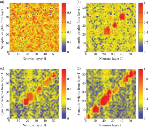
The emergence of this diagonal in the synaptic weight matrix is a phenomenon of note. Even though the initial values of all connections were randomly set, during the LTP learning process it was possible to observe how the weights reinforced in a consistent way, shown by the red-colour activity. We discuss this later in Section 4.2. It is worth noting though that the diagonal is formed as a result of the topological correspondence of the two different sensory modalities. As pointed out in Section 2, this correspondence is an emergent phenomenon of the forward model predictions.

4.1.2. Testing phase

To test the performance and robustness of the system, two navigation tasks were performed in two different mazes as shown in Figure 13. In both situations the agent moves towards the end of the corridor. In the first task (Figure 13(a)), the robot navigates through a narrow ‘S-shaped’ corridor. In the second task (Figure 13(b)) the robot undertakes an avoiding behaviour as obstacles appear in its visual field.

Figure 13. Experimental settings showing two different environments. (a) Maze 1: S-shaped corridor. (b) Maze 2: corridor with obstacles on both sides.

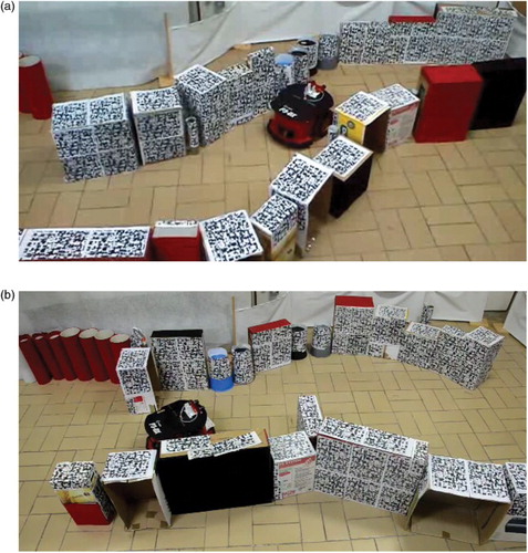
The behaviour observed in both tasks is undertaken using only the visual modality in an anticipatory way; i.e. only the visual input (MDV) produces a motor change so as to navigate safely by remaining away from obstacles. This change is due to neural activations in the controlling network according to incoming visual patterns. Our claim is that the behaviour is anticipatory in that the current stimulus represents a visual pattern that, during the learning phase, was associated with a future bumper state which implied a possible collision. Videos showing experiments can be found in http://youtu.be/M96uVu5CPlU and in http://youtu.be/wrRg1LQcoOA.

4.2. Discussion of the first experiment

In order to give a quantitative measure of the behaviour of the system in different stages of the learning process, we plotted the power signal of the difference between left (M_l) and right (M_r) motor values. This gives an account of the performance of the robot in terms of its manoeuvres and their timely application during the execution as will be explained later. A non-zero or increasing power implies a change in direction (rotational motions), whereas zero or decreasing behaviour means movements in the same direction.

This power is computed by where N is the total number of steps executed by the robot.

Figure 14 shows this signal for both mazes. In Figure 14(a) it can be observed that curves (a) and (b) (corresponding to the weight matrices in Figure 12(a) and (b), respectively) stop at about step 15, showing that the robot crashes around mid-way through the corridor. In contrast, the behaviour described by curves (c) and (d) (corresponding to weight matrices in Figure 12(c) and (d), respectively) shows that the robot reaches the end of the corridor. The situation is similar for the second maze. However, when using the weight matrix in Figure 12(a), the presence of an obstacle directly in front causes the robot to crash much earlier in the maze. In this situation, only the fully trained network is capable of travelling the whole corridor, as shown by curve (d).

Figure 14. Power signals of robot direction change corresponding to maze 1 (left plots) and maze 2 (right plots) for one individual. Curves labelled (a) correspond to the case where the individual uses an association matrix with random weights (see Figure 12(a)), in both cases the agent fails to reach the end of the maze. In contrast, curves labelled (d) correspond to the case where the individual uses an association matrix with strong weights around the main diagonal (see Figure 12(d)). Curves (b) and (c) correspond to individuals using an association matrix configuration corresponding to Figure 12(b) and (c), respectively. Therefore, it can be seen that the individual only copes with both mazes provided that the association matrix has stable weights around the main diagonal.

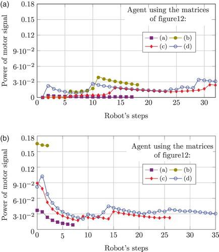
Regarding the anticipation process acquired during the learning phase, a telling example is the behaviour observed in Figure 14(a), referring to the event at about step 10. Using the matrix of Figure 12(b), the agent reacts with a high power early in the maze. However, this anticipatory behaviour results in a future collision at step 18. As the learning process develops, the robot undertakes the same turn but this time one step earlier and with less power, as shown by curve (d) in Figure 14(a). For both mazes, a fine tuning of the control is evident, and it can be observed that only a fully trained matrix allows one to perform collision-free trajectories.

Configuration and topology of the mazes are captured neatly in both plots in Figure 14. In maze 1, presenting soft corners and curves, the fully trained network performs soft changes in the direction as necessary to avoid crashing. However, in maze 2, that presents fully frontal obstacles and sharp curves, the robot requires stronger motor signals, meaning sharp changes in the direction.

In order to appreciate the constraints that the environment imposed to the robot and its performance under those conditions, Figure 15 shows two pairs of plots representing sonar readings in two distinct ways.

Figure 15. Experimental data of one individual using the fully trained association matrix. (a) and (b) Sonar topography for mazes 1 and 2, respectively. At each step, the maps represent the configuration of obstacles around the robot within an 800-mm region, which corresponds to the distance covered by an LTP. The blue valley means no obstacle within this region. Obstructions in the frontal zone (sonars 3 and 4) may appear at each step whenever obstacles ahead fall into this region. (c) Performance metrics for Maze 1 (S-shaped). The maze width curve describes the absolute free-space aperture, showing that the first half is wider than the second. As the robot reaches the end of the maze, the distance to obstacles is shorter, correlated with a narrower gap. (d) Performance metrics for Maze 2 (Corridor). The maze width curve describes the aperture and the presence of obstacles along the corridor. Between steps 9 and 17 the first obstacle appears, and the second one shows up between steps 24 and 29.

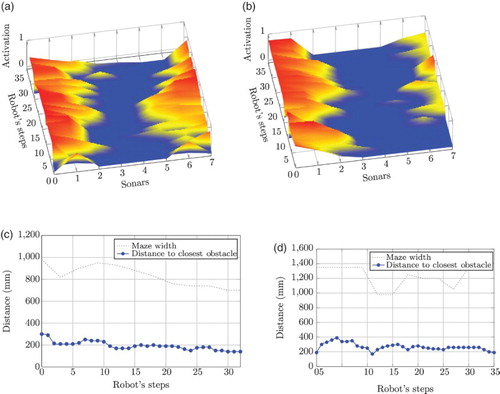
On one hand, Figure 15(a) and (b) depicts topography maps of sonar readings. These maps show sonar values of the eight sensors as the robot moves throughout the mazes using the fully trained weight matrix. The readings were normalised in the range [0, 1], where 1 represents a collision state (red-coloured area) and 0 no presence of obstacles in a radius of 800 mm around the robot (blue-coloured area). This threshold value corresponds to 5 robot steps which is the maximum number of steps executed during LTP in the training phase.

Figure 15(a) depicts the sonar activation map while navigating through the S-shaped maze. The topography of the map reveals the spatial characteristics of the environment. We can see a shallow valley centred at the front of the robot (represented by sensors 3 and 4). The robot makes the necessary turns to keep that valley in the centre, as that ensures a collision-free trajectory. For maze 2, Figure 15(b) shows a wider valley accounting for a wider corridor. The structure of the corridors can be seen from the variation of the outward sensor readings. It is important to keep in mind that these maps are robot-centred and therefore do not directly reflect the shape of the mazes as seen in world coordinates. Still, the centre valley in both figures shows that the robot copes well with obstacles.

On the other hand, Figure 15(c) and (d) shows a performance metric obtained from sonar readings. In these figures we plotted, at every step, the distance to the closest obstacle together with the edge profile of the corresponding maze. The size of the gap at every step corresponds approximately to the width of the path along the maze. As can be seen the first maze is narrower than the second. The plots show that the agent kept a similar average distance from obstacles.

4.3. Different individuals

4.3.1. Training phase

Another test of the system was performed using different individuals. The idea is to obtain five different individuals, equipped with the same machinery but learning under different conditions. Therefore, they all were trained using the same architecture, but each one faced small variations on the distribution of obstacles in the training arena. The obstacles were placed at different distances from the centre of the setting, allowing for different lengths of LTP.

All individuals started with different random weights and distinct random initial positions. The variation on the obstacles distribution, the random initial position and the different number of steps of LTP have a direct effect on the final configuration of association weights (e.g. Figure 16 depicts these weights for two different individuals namely 1 and 5 who exhibited the most contrasting behaviour in the testing phase).

Figure 16. Synaptic weights (matrix W) after 300 steps of LTP for individual 1 (a) and 100 steps for individual 5 (b).

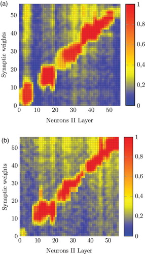
These small variations are sufficient to produce differences in behaviour during a navigation task; the results are discussed in the next section.

4.3.2. Testing phase

Figure 17 depicts the behaviour of five different individuals after being trained. During the test phase they all travelled through the same maze, similar to the one shown in Figure 13(b). All agents started with the same initial conditions.

Figure 17. The behaviour of five individuals during the test phase of experiment 2. (a) The maximum value of the MDV is highlighted for individuals 1 and 5. This signal codes the presence of obstacles in the visual field, closer obstacles imply a higher value. All signals are correlated as the individuals travelled along the same maze with same initial conditions. (b) Corresponding motor power signals. Individuals 1 and 5 show a neat difference starting halfway through the maze.

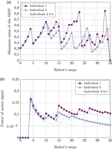
Figure 17(a) shows, for each step, the maximum MDV value when the agents travelled through the maze. Two typical individuals are shown in solid lines, the rest are plotted in grey. These plots sketch the characteristics of the path followed by all members: the higher the MDV value, the closer the robot came to an obstacle.

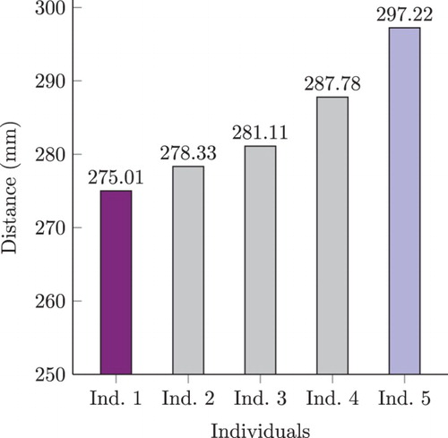
Figure 17(b) shows computations of the corresponding motor-difference power signal. In general, the behaviour of the MDV is correlated to power fluctuations. However, the power signals of members 1 and 5 show a neat difference starting halfway through the maze. It would appear that, by a smoother and timely manoeuvre, individual 5 sorted out the constraints of the environment better than the rest of the group. This was corroborated, the performance of all agents was analysed by computing their average closest proximity to obstacles. This is depicted in Figure 18. Individual 5 actually performs better than any other one under this metric. Although very intriguing, the research of the causal implications of this performance is out of the scope of this work. Still, all individuals were capable of safely navigating through the full corridor, showing the robustness of the model.

Figure 18. Maximum proximity for test 2. Average closest proximity for the five individuals in the test phase of experiment 2. It is the average of the closest distance to an obstacle as reported by sonar sensors during all steps in the trajectory. Individual 5 performed the best as it remained the most distant from obstacles during its trajectory. Coloured bars correspond to the same individuals highlighted in Figure 17.

5. Discussion and conclusions

Cognitive mechanisms in humans, involving the motor control system, are far from being completely understood. Our work constitutes an attempt to validate the concept of mental imagery in a computational implementation.

We propose an artificial anticipatory mechanism built upon an off-line multi-modal sensory association process. We took into consideration architectural constraints and mental imagery features such as the reinforcement of sensorimotor coordination and a motor control conditioning function. Extensive work found in the literature about mental training and its relation to the motor system supports our proposal (e.g. see Di Nuovo et al., 2013; Jeannerod, 1995; Jeannerod, 2001).

Our work is related to those initiatives aiming at modelling brain functions. Herreros & Verschure (2013), for instance, provide a computational model of the cerebellum function involved in Avoidance Learning, by coupling a reactive and adaptive layers of control. This model acts similar to the CS–US association of classical conditioning, by adding a conditioned response (CR) coming from the adaptive layer to the reactive response. To cope with time constraints, Brandi et al. (2013) proposed to extend this cerebellum model by chaining several associations, using one CR as the CS for the learning of the next action. They hypothesise that this recurrence might be established through the Nucleo-Pontine Projections (NPPs), a set of connections linking the input and output structures of the cerebellum.

Also, many predictive architectures found in the literature are used in similar experimental contexts with mobile robots. Contrary to other work, where metric or world position coordinates are used (e.g. Hoffmann, 2007), we take the disparity map as an implicit visual (distance) sensor. The idea is to provide the agent with cognitive tools allowing it to acquire a physical embodied notion of distance (in this case a dangerous distance to obstacles).

Moreover, in cognitive robotics, the biologically inspired hebbian learning process has been used as a mechanism to relate perception and action in robots, in order to obtain complex behaviours in navigational tasks or goal-directed actions (Verschure et al., 1992; Wang et al., 2009). Also, biologically inspired computational models have been proposed in the literature to achieve predictive mechanisms (Ruesch et al., 2012). In a work closely related to ours, McKinstry et al. (2006) present an association mechanism to replace reflexes with a predictive controller. The learning process occurs while executing overt actions during a navigation task. In this and similar applications, agents, learn every time an action is overtly executed.

However, none of these approaches use internal simulations. Likewise, research on implementations of forward models for navigation (e.g. Kaiser et al., 2010; Lara et al., 2007b, and others) has not presented a further control strategy. Our method does not seek to improve the prediction or the forward model. We aim at fusing, in a computational way, internal simulations via forward models and off-line hebbian learning, in what we describe as an artificial mental imagery process. This is precisely what we believe to be the most interesting part of our work and our main contribution.

In order to reach our goal, we use a system of neural networks coding a forward model acting as a predictor. This model provides the system with visual and tactile stimuli predictions during forward motions. Then we apply hebbian learning to the system connections during internal simulations of the predicted sensorimotor flows.

As a result of consecutive iterations of this process, the association between two distinct modalities yields a structured topology even without overt actions. This topology improved during learning, endowing the robot with a controlling mechanism triggering an UR through a CS.

The mechanism is anticipatory in that current stimuli represent a visual pattern that, during the learning phase, was associated with a future bumper state which implied a possible collision.

We do not want to delve into a discussion about the non-representational character of this model. The controller allows the robot to enact a collision avoidance behaviour only from visual information, but no future representation of that collision in the visual field takes place at any time. In any case, the representation is modal in as much as the controlling network constitutes in itself a grounded mechanism.

We tested our model in a physical Pioneer 3-DX robot, by letting it navigate in two different mazes, imposing different constraints to the robot in order to perform collision-free trajectories. Once the off-line learning process has reached a stability state, the robot is capable of coping with environmental challenges.

The experiments showed that the avoiding behaviour is controlled by anticipation of tactile consequences previously coded together with the visual modality. In this respect, a new control strategy showing an anticipatory feature emerges from a multi-modal association process taking place during the internal simulation of sensorimotor cycles.

We believe that our work represents a proof of concept and an important piece in the paradigm of computational grounded cognition (Pezzulo et al., 2012). Hopefully, our work offers an underpinning mechanism in cognitive robotics for the study of motor control strategies based on internal simulations. These may be akin to the mental imagery process known in humans, opening thus interesting pathways to the construction of upper-level grounded cognitive abilities.

Notes

1. The idea of off-line training via simulated ‘experience’ is not new and can be traced back to DYNA (Sutton, 1991), under the classical framework of reinforcement learning. However, computational modelling of human motor cognition, in non-representational frameworks (i.e. where sensory input readings are not mediated by state space representations), is still an open research vein.

2. These include the study of learning through imitation (Dearden & Demiris, 2005), action recognition and execution (Akgun et al., 2010; Schillaci et al., 2012), and navigation (Lara et al., 2007a; Möller & Schenck, 2008; Ziemke et al., 2005).

3. This weight update iterative process is analogous to the reinforcement effect we have mentioned, which should not be mistakenly associated with reinforcement learning techniques commonly used in robotics for planning and control.

4. This variation in the number of steps will be explained in Section 4.1.

References

- Akgun, B., Tunaoglu, D., & Sahin, E. (2010, November 5–7). Action recognition through an action generation mechanism. International conference on epigenetic robotics (EPIROB), Örenäs Slott, Sweden.
- Asada, M., Hosoda, K., Kuniyoshi, Y., Ishiguro, H., Inui, T., Yoshikawa, Y., … Yoshida, C. (2009). Cognitive developmental robotics: A survey. IEEE Transactions on Autonomous Mental Development, 1(1), 12–34. doi: 10.1109/TAMD.2009.2021702
- Barsalou, L. W. (2008). Grounded cognition. Annual Review of Physiology, 59, 617–645.
- Brandi, S., Herreros, I., Sánchez-Fibla, M., & Verschure, P. (2013). Learning of motor sequences based on a computational model of the cerebellum. In N. Lepora, A. Mura, H. Krapp, P. Verschure & T. Prescott (Eds.), Biomimetic and biohybrid systems (Vol. 8064, pp. 356–358). Berlin: Springer.
- Butz, M. V., Sigaud, O., & Gerard, P. (2002). Internal models and anticipations in adaptive learning systems. In P. Gerard, M. V. Butz & O. Sigaud (Eds.), Adaptive behaviour in anticipatory learning systems (abials’02) (pp. 282–301), Heidelberg: Springer.
- Dadds, M. R., Bovbjerg, D. H., Redd, W. H., & Cutmore, T. R. H. (1997). Imagery in human classical conditioning. Psychonomic Bulletin, 122(1), 89–103. doi: 10.1037/0033-2909.122.1.89
- Dearden, A., & Demiris, Y. (2005). Learning forward models for robots. International joint conferences on artificial intelligence (p. 1440), Edinburgh.
- Di Nuovo, A. G., De La Cruz, V. M., & Marocco, D. (2012). Mental imagery for performance improvement in humans and humanoids. In A. G. Di Nuovo, V. M. De La Cruz & D. Marocco (Eds.), Proceedings of the SAB workshop on artificial mental imagery in cognitive systems and robotics, Odense, Denmark (pp. 1–5). Plymouth: Plymouth University.
- Di Nuovo, A. G., Marocco, D., Di Nuovo, S., & Cangelosi, A. (2013). Autonomous learning in humanoid robotics through mental imagery. Neural Networks, 41, 147–155. doi: 10.1016/j.neunet.2012.09.019
- Driskell, J. E., Cooper, C., & Moran, A. (1994). Does mental practice enhance performance? Journal of Applied Psychology, 79(4), 481–492. doi: 10.1037/0021-9010.79.4.481
- Escobar, E., Hermosillo, J., & Lara, B. (2012). Self body mapping in mobile robots using vision and forward models. CERMA 2012, Cuernavaca. IEEE Computer Society.
- Frank, C., Vogel, L., & Schack, T. (2012). Mental imagery and mental representation – how to use biological data on technical platforms. In A. G. Di Nuovo, V. M. Di De La Cruz & D. Marocco (Eds.), Proceedings of the SAB workshop on artificial mental imagery in cognitive systems and robotics, Odense, Denmark (pp. 15–18). Plymouth: Plymouth University.
- Grush, R. (2004). The emulation theory of representation: Motor control, imagery, and perception. Behavioral and Brain Sciences, 27, 377–342.
- Hebb, D. (1949). The organization of behavior A neuropsychological theory. Lawrence Erlbaum Associates.
- Herreros, I., & Verschure, P. F. M. J. (2013). Nucleo-Olivary inhibition balances the interaction between the reactive and adaptive layers in motor control. Neural Networks, 47, 64–71. Retrieved from http://dx.doi.org/10.1016/j.neunet.2013.01.026 (Special Issue). doi: 10.1016/j.neunet.2013.01.026
- Hoffmann, H. (2007). Perception through visuomotor anticipation in a mobile robot. Neural Networks, 20, 22–33. doi: 10.1016/j.neunet.2006.07.003
- Jeannerod, M. (1995). Mental imagery in the motor context. Neuropsychologia, 33(11), 1419–1432. Retrieved from http://www.sciencedirect.com/science/article/pii/002839329500073C (The Neuropsychology of Mental Imagery). doi: 10.1016/0028-3932(95)00073-C
- Jeannerod, M. (2001). Neural simulation of action: A unifying mechanism for motor cognition. Neuroimage, 14(1), S103–S109. doi: 10.1006/nimg.2001.0832
- Kaiser, A., Schenck, W., & Möller, R. (2010, September 9). Mental imagery in artificial agents. Workshop new challenges in neural computation 2010, Bielefeld, Germany, pp. 25–32.
- Kosslyn, S. M. (1994). Image and brain. Cambridge, MA: MIT Press.
- Kosslyn, S. M., Thompson, W. L., & Ganis, G. (2006). The case for mental imagery. New York, NY: Oxford University Press.
- Lara, B., Rendon, J. M., & Capistran, M. (2007a, November 8–9). Prediction of multi-modal sensory situations, a forward model approach. Proceedings of the fourth IEEE Latin America robotics symposium (Vol. 1), Monterrey, Mexico.
- Lara, B., Rendon, J. M., & Capistran, M. (2007b). Prediction of multi-modal sensory situations, a forward model approach. Adaptive Behaviour, 8, 9.
- McKinstry, J. L., Edelman, G. M., & Krichmar, J. L. (2006). A cerebellar model for predictive motor control tested in a brain-based device. Proceedings of the National Academy of Sciences of the United States of America, 103(9), 3387–3392. doi: 10.1073/pnas.0511281103
- Miall, R. C., & Wolpert, D. M. (1996). Forward models for physiological motor control. Neural Networks, 9, 1265–1279. doi: 10.1016/S0893-6080(96)00035-4
- Möller, R., & Schenck, W. (2008). Bootstrapping cognition from behaviour – a computerized thought experiment. Cognitive Science, 32(3), 504–542. doi: 10.1080/03640210802035241
- Moulton, S. T., & Kosslyn, S. M. (2009). Imagining predictions: Mental imagery as mental emulation. Philosophical Transactions of the Royal Society of London. Series B: Biological Sciences, 364, 1273–1280.
- Pavlov, I., & Anrep, G. (2003). Conditioned reflexes. Mineola, NY: Dover Publications. (Original work published 1927)
- Pezzulo, G. (2008, June). Coordinating with the future: The anticipatory nature of representation. Minds and Machines, 18(2), 179–225. doi: 10.1007/s11023-008-9095-5
- Pezzulo, G., Barsalou, L. W., Cangelosi, A., Fischer, M. H., McRae, K., Spivey, M. J., et al. (2012). Computational grounded cognition: A new alliance between grounded cognition and computational modeling. Frontiers in Psychology, 3, 612. doi: 10.3389/fpsyg.2012.00478
- Riedmiller, M., & Braun, H. (1993, March 28–April 1). A direct adaptive method for faster backpropagation learning: The RPROP algorithm. IEEE international conference on neural networks, San Francisco, CA, Vol. 1, pp. 586–591.
- Ruesch, J., Ferreira, R., & Bernardino, A. (2012). Predicting visual stimuli from self-induced actions: An adaptive model of a corollary discharge circuit. IEEE Transactions on Autonomous Mental Development, 4(4), 290–304. doi: 10.1109/TAMD.2012.2199989
- Schacter, D. L., Addis, D. R., & Buckner, R. L. (2007). Remembering the past to imagine the future: The prospective brain. Nature Reviews Neuroscience, 8, 657–661. doi: 10.1038/nrn2213
- Schenck, W., Hasenbein, H., & Möller, R. (2012). Detecting affordances by mental imagery. In A. G. Di Nuovo, V. M. De La Cruz, & D. Marocco (Eds.), Proceedings of the SAB workshop on artificial mental imagery in cognitive systems and robotics (pp. 15–18). Plymouth: Plymouth University.
- Schillaci, G., Lara, B., & Hafner, V. (2012). Internal simulations for behaviour selection and recognition. In A. Salah, J. Ruiz-del Solar, C. Meriçli, & P.-Y. Oudeyer (Eds.), Human behavior understanding (Vol. 7559, pp. 148–160). Berlin: Springer.
- Sutton, R. S. (1991). Dyna, an integrated architecture for learning, planning, and reacting. SIGART Bulletin, 2(4), 160–163. doi: 10.1145/122344.122377
- Tikhanoff, V., Cangelosi, A., & Metta, G. (2011). Integration of speech and action in humanoid robots: Icub simulation experiments. IEEE Transactions on Autonomous Mental Development, 3(1), 17–29. doi: 10.1109/TAMD.2010.2100390
- Verschure, P. F., Kröse, B. J., & Pfeifer, R. (1992). Distributed adaptive control: The self-organization of structured behavior. Robotics and Autonomous Systems, 9(3), 181–196. doi: 10.1016/0921-8890(92)90054-3
- Wang, Y., Wu, T., Orchad, G., Dudek, P., Rucci, M., & Shi, B. E. (2009). Hebbian learning of visually directed reaching by a robot arm. Biomedical circuits and systems conference, 2009, BioCAS 2009, Beijing. IEEE, 205–208.
- Wilson, M. (2002). Six views of embodied cognition. Psychonomic Bulletin and Review, 9, 625–636. doi: 10.3758/BF03196322
- Wolpert, D. M., Ghahramani, Z., & Flanagan, J. R. (2001). Perspectives and problems in motor learning. Trends in Cognitive Sciences, 5(11), 487–494. doi: 10.1016/S1364-6613(00)01773-3
- Ziemke, T., Jirenhed, D.-A., & Hesslow, G. (2005). Internal simulation of perception: A minimal neuro-robotic model. Neurocomputing, 68, 85–104. doi: 10.1016/j.neucom.2004.12.005