Semantic segmentation of high-resolution remote sensing images using fully convolutional network with adaptive threshold

ABSTRACT

Semantic segmentation is an important method to implement fine-grained semantically understand for high-resolution remote sensing images by dividing images into pixel groupings which can then be labelled and classified. In the field of computer vision (CV), the methods based on fully convolutional network (FCN) are the hotspot and have achieved state-of-the-art results. Compared with popular datasets in CV such as PASCAL and COCO, class imbalance is a problem for multiclass semantic segmentation in remote sensing datasets. In this paper, an FCN-based model is proposed to implement pixel-wise classifications for remote sensing image in an end-to-end way, and an adaptive threshold algorithm is proposed to adjust the threshold of Jaccard index in each class. Experiments on DSTL dataset show that the proposed method produces accurate classifications in an end-to-end way. Results show that the adaptive threshold algorithm can increase the score of average Jaccard index from 0.614 to 0.636 and achieve better segmentation results.

KEYWORDS:

• Semantic segmentation
• remote sensing images
• fully convolutional network
• class imbalance
• adaptive threshold

1. Introduction

Semantic segmentation (also named image classification in remote sensing) is the pixel-wise classification of an image and is an important task for numerous applications of object recognition (Forestier et al., 2012). With the rapid development of Remote Sensing (RS) technology, the RS imagery produced by high-resolution remote sensing satellites (such as IKONOS, SPOT-5, WorldView and Quickbird) have more abundant information to extract features and recognition ground object than the low-resolution remote sensing imagery. Many artificial objects that are difficult to be recognised in the past are now available to be detected (Cheng & Han, 2016). Semantic segmentation has been widely studied in computer vision (CV) and remote sensing, mainly using shallow features that were hand-engineered by skilled people who have experience in the field and also often required domain-expertise (Girshick et al., 2014). This also means that if the conditions change even slightly, a framework which works well in a given task may fail in another task and the whole feature extractor might have to be rewritten from scratch, which is very time-consuming and expensive. These disadvantages led researchers in the field looking for a more robust and effective approach.

In recent years, convolutional neural networks (CNNs) are widely used in various image recognition problem and achieve state-of-the-art results (Simonyan & Zisserman, 2014). In 2012, Krizhevsky, Sutskever, and Hinton (2012) won the ILSVRC competition by a model with 7-layer CNN named AlexNet, and that result opened the floodgates to new research in the field with the name “deep learning”. Concept of convolutional layer introduced from CNN uses two methods to greatly reduce the number of parameters: local receptive field and parameter sharing. Local receptive field is a principle learned from human visual that the pixels in an image have more relevant with the adjacent pixels. Instead of having each neuron receive connections from all neurons in the previous layer, CNNs use a receptive field-like layout in which each neuron receives connections only from a subset of neurons in the previous (lower) layer. The use of receptive fields in this fashion is thought to give CNNs an advantage in recognising visual patterns when compared to other types of neural networks. Parameter sharing scheme is used in Convolutional Layers to control the number of parameters. Generally, the statistical features of part of the image are considered same with the other parts. So that the convolution kernel is used as a feature extraction method regardless of the position, pool layer (Boureau, Ponce, & LeCun, 2010) is used to represent the implied invariance from transformation of the image.

A preliminary set of experiments fusing CNNs obtains state-of-the-art results for the well-known UCMerced dataset (Marmanis et al., 2016a; Penatti, Nogueira, & Santos, 2015; Zhong et al., 2017). The results of these researches show that the CNNs can be generalised to the field of remote sensing imagery and obtain better results than the traditional methods. Recently CNNs have emerged as the leading modeling tools for semantic segmentation in general and have had an increasing impact in remote sensing (Garcia-Garcia et al., 2017). In ISPRS semantic segmentation challenge (Semantic Labeling Contest[EB/OL], 2018), CNNs are dominating and are shown to provide the best performing model (Marmanis et al., 2016b). Fully convolutional network (FCN) (Shelhamer, Long, & Darrell, 2017) directly learn a mapping from image pixels to class labels by replacing the fully connected layer of CNNs with a convolutional layer.

In this paper, we employ a framework to perform semantic segmentation for HRRS image based on FCN. Our paper makes three major contributions: (1) an FCN model is applied for semantic segmentation of remote sensing images; (2) an adaptive threshold algorithm is proposed to get better result for class with no enough training data; (3) we experiment with DSTL dataset and obtain outstanding performance.

2. Related work

2.1. Simple classification-based methods

As early as 1989, researchers tried to apply machine learning methods to solve pixel-level classification of remote sensing images (Decatur, 1989). Early approaches use directly the values at different spectral bands as features. Then hand-crafted features extracted from local spectral and textural such as Colour Histograms, HOG, SIFT (Zhang, Zhang, & Du, 2016) are used. The Bayes’ classifier is one of simplest and most popular methods to image classification (Bischof, Schneider, & Pinz A, 1992). Due to the need to learn such highly nonlinear decision boundaries, applications of machine learning to high-resolution imagery have relied on more sophisticated classifiers such as SVMs (Mountrakis, Im, & Ogole, 2011), random forests (Pal, 2005) and various types of boosting (Atkinson & Lewis, 2000). With the improvement of resolution, the approaches of using the values of multiple bands and hand-crafted features (such as local spectral and textural features) cannot provide enough information to classifier. Many unsupervised and supervised feature learning methods such as sparse coding, Restricted Boltzmann Machines (Han et al., 2015) and CNN are used in recent researches that show significantly improve both precision and recall.

2.2. CNN-based methods

Traditional CNNs are usually used for classification task, and the output of classification is discrete class label. Patch-based classification algorithm proposed by Volodymyr Mnih (2013) is a traditional CNN-based framework to implement semantic segmentation. It extracts the image patch near each pixel and takes the patch as input image of a CNN model to train the model or predict the label of the pixel. A sliding window is used to extract patches around all pixels in the input image. CNNs implemented on modern GPUs can be used to efficiently learn highly discriminative image features. Patch-based classification algorithm achieves higher classification accuracy than simple classification (Sharma et al., 2017). The disadvantages of this method are large memory requirement, long processing times, and limitation of the size of the receptive field.

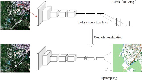
As is shown in Figure 1, there are several fully connected layers in a classic CNN after the convolutional layers, mapping the feature map generated by the convolutional layer into a fixed-length feature vector. The final classification probabilities are computed by applying a sigmoid function or softmax function to the output of the last layer. Unlike classic CNNs, which use connected layers to obtain a fixed-length feature vector for classification after a convolutional layer (fully connected layer and softmax output), FCN replaces the last fully connected layers of CNN with a convolutional layer (Shelhamer et al., 2017). In this method, a transposed convolutional layer is employed to perform up-sampling the feature map. This operation is essential in order to produce outputs of the same spatial dimensions as the inputs. The output of FCN is a picture that has already been labelled.

Figure 1. Difference between patch-based CNN and FCN (Top: patch-based CNN, down: FCN model).

2.3. FCN-based methods

In view of problems of patch-based classification algorithm, Jonathan Long (Shelhamer et al., 2017) proposed a framework based on FCN for image segmentation. FCN removes the fully connected layer in CNNs and tries to recover the specific classification of each pixel from abstract features. FCN is an end-to-end model, input and output of it are both images. In FCN, the shallow layers with high-resolution are used to solve the problem of pixel positioning, the deep layers with low-resolution are used to solve the problem of pixel classification. Due to its ability of fitting any input and output size of segmentation map and its more effective compared to the traditional methods, FCN model becomes the research hotspot in the field of semantic segmentation. Many FCN-based models such as SegNet (Badrinarayanan, Kendall, & Cipolla, 2017), U-Net (Ronneberger, Fischer, & Brox, 2015), DeconvNet (Noh, Hong, & Han, 2015), Deeplab (Chen et al., 2018) and so on have been proposed to improve the segmentation performance by introducing the principles of atrous convolution, atrous spatial pyramid pooling, conditional random field. Increasing benchmark datasets (such as PASCAL VOC2012, MSCOCO, ADE20K, Cityscapes) help researches develop better machine learning system for semantic segmentation (Garcia-Garcia et al., 2017).

Recently, more and more researches have been focused on designing and applying FCN model for semantic segmentation tasks in remote sensing (Zhao, Feng, Wu, & Yan, 2017). Muruganandham (Muruganandham, 2016), (Wei, Wang, & Xu, 2017), (Kaiser, 2016) proposed FCN-based model for road and building extraction. Kampffmeyer M (Kampffmeyer, Salberg, & Jenssen, 2016) combine patch-based and pixel-to-pixel approaches to segmentation small objects. Kemker R (Kemker & Kanan, 2017) train models initialised with synthetic imagery to avoid over-fitting. Some researches focus on developing FCN-based model and post-processing method to improve segmentation (Fu et al., 2017; Liu et al., 2017; Maggiori et al., 2016; Saito, Yamashita, & Aoki, 2016). Benchmark datasets (such as Mass Building and Mass Roads (Mnih, 2013), Inria Aerial Image Labeling dataset (Maggiori et al., 2017), IEEE GRSS Data Fusion Contest dataset (Tuia et al., 2017), DSTL Satellite Imagery Feature Detection dataset (DSTL Satellite Imagery Feature Detection, 2017), ISPRS benchmark datasets (Semantic Labeling Contest[EB/OL], 2018), RIT-18 (Kemker & Kanan, 2017) and SIRI-WHU (Ma, Zhong, & Zhang, 2015)) provided by research institutes all over the world greatly support future study.

3. Proposed FCN-based method with adaptive threshold

3.1. Architecture

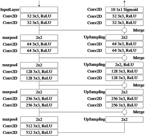
The U-NET model which won the EM image segmentation competition in ISBI 2015 is currently the most easily scalable/sizeable FCN architecture for semantic segmentation. The network works well with very few training images and yields more precise segmentations, has shown the potential in various fields. Because of the advantages as above, U-NET model is used to be foundation framework in this paper. U-Net is regarded as a typical model with encoder-decoder structure. The encoder reduces the spatial dimension of by pooling layer and the decoder gradually restores the detail and spatial dimension of the object by upsampling layer. The architecture of Modified U-Net used in this paper is shown in Figure 2. It is a symmetrical structure consists of contraction path in the left part and extension path in the right part. The contraction path is similar to the traditional convolutional network, in which the maxpool layer double the number of feature channel after two convolutional layers with 3 × 3 convolution kernel. To do upsampling operators, feature map in the extension path merge with the corresponding feature map in the contraction path. Process of upsampling is an up-convolution with 2 × 2 convolution kernel. Following by two convolutional layers with 3 × 3 convolution kernel to make up for the lack of location information lost by the maxpool layers. The normalisation (batch-normalisation) operation is completed during downsampling path, following by dropout operation. In this model, ReLU (Rectified Linear Units) is activation function used in all of the convolutional layer, Adam (Adaptive Moment Estimation) is optimiser, cross entropy function is the loss function, Average Jaccard Index (also known in literature as Intersection-over-Union) is the evaluation metric.

Figure 2. The architecture of our model.

3.2. Data pre-processing

3.2.1. Data standardisation

The remote sensing image data is an integer, the parameters of the neural network and the output of activation function are usually initialised to a random number between (0,1). The data standardisation method is used to avoid the abnormal gradient. In this paper, z-score normalisation algorithm is used to adjust the pixel value of the input image to approximate Normal distribution is conducive to activation and gradient descent process. μ and σ represent the mean and standard deviation of X/Max, the normalisation formula is shown as below. (1) $X_{\mathrm{out}}=\frac{\left(X/\text{Max}\right)-\mu }{\sigma }.$(1)

3.2.2. Data augmentation

The purpose of data augmentation is to generate new sample instances, and when the training samples are few, data augmentation is very useful for improving the robustness of the network. It is no need to do data augmentation for the validation set and the test set. For remote sensing imagery, there are many popularly used methods of data augmentation such as colour jittering, principal component analysis (PCA) jittering, random resize, horizontal/vertical flip, shift, rotation/reflection, noise, cutting, switching frequency band and so on. Since most remote sensing image are orthophoto images, the changes mainly reflect in direction and scale. However, the images in data set used in this paper are the same resolution, there is no big scale change, so only three common augmentation methods are used: horizontal/vertical flip, rotation, and random crop. The image patches are extracted with size 160 × 160 from the original images with 50% of overlap and flipped horizontally and vertically. After data augmentation, the dataset is augmented by 14 times.

3.3 Model training

3.3.1. Optimisation

Stochastic Gradient Descen is the most common optimiser in CNNs, but it has some problems in finding the appropriate learning rate and easily converging to local optimum. In this paper, Adam (Kingma & Ba, 2014) (Adaptive Moment Estimation) optimiser is used as learning strategy to calculate the adaptive learning rate of each parameter. Adam optimiser adjusts the learning rate of each parameter according to the first moment estimation and the second moment estimation of its gradient function of loss function. Adam optimiser runs fast and can correct the problems of learning rate disappears, slow convergence speed and great fluctuation of the loss function. Adam optimiser is shown as below formulas. (2) ${\hat{m}}_t=m_t/1-{\beta }_1^t,$(2) (3) ${\hat{v}}_t=v_t/1-{\beta }_2^t,$(3) (4) ${\theta }_{t+1}={\theta }_t-\frac{\eta }{\sqrt{{\hat{v}}_t}+\epsilon }{\hat{m}}_t.$(4) Formula (2) represents first moment deviation, formula (3) represents second moment deviation. $\eta$ is step, $\epsilon$ is a little constant (default value is ${10}^{-8}$).

3.3.2. Loss function

In mathematical optimisation, statistics, econometrics, decision theory, machine learning and computational neuroscience, a loss function or cost function is a function that maps an event or values of one or more variables onto a real number intuitively representing some “cost” associated with the event. An optimisation problem seeks to minimise a loss function. An objective function is either a loss function or its negative (in specific domains, variously called a reward function, a profit function, a utility function, a fitness function, etc.), in which case it is to be maximised. The energy function is computed by a cross entropy loss function. Formula of it is shown as below. (5) $-\sum (y_{\mathrm{true}}\log y_{\mathrm{pred}}+(1-y_{\mathrm{true}})\log (1-y_{\mathrm{pred}}\left)\right).$(5)

3.3.3. Evaluation metric

In order to evaluate the performance of the algorithm, results of the model should be compared to the ground truth. In this paper, Average Jaccard Index is used to predict the value and the true value. The Jaccard index, also known as Intersection over Union and the Jaccard similarity coefficient, is a statistic used for comparing the similarity and diversity of sample sets. The Jaccard coefficient measures similarity between finite sample sets and is defined as the size of the intersection divided by the size of the union of the sample sets. (6) $\text{score}=\frac{1}{N}\sum _{i=1}^N\text{jaccar}{\text{d}}_i=\frac{1}{N}\sum _{i=1}^N\frac{\text{T}{\text{P}}_i}{\text{T}{\text{P}}_i+\text{F}{\text{P}}_i+\text{F}{\text{N}}_i},$(6) $N$ is the number of classes, $\text{TP}$ is true positive, $\text{FP}$ is false positive, $\text{FN}$ is false negative.

3.3.4. Fine-tuning

Transfer learning strategies depend on various factors, but the two most important ones are the size of the new dataset, and its similarity to the original dataset. Fine-tuning (Hentschel, Wiradarma, & Sack, 2016) allows us to bring the power of state-of-the-art DCNN models to new domains where insufficient data and time/cost constraints might otherwise prevent their use. This approach achieves a significant improvement of average accuracy and improves the state-of-the-art of image-based medical classification.

3.4 Adaptive threshold

Output of FCN is a 4-d tensor, includes probabilities of every pixels in m input images with size $x\times y$ belong into n classes. After training finished, a threshold $t$ should be set up to decide whether a pixel falls in the predefined category. If $p>t$ the pixel can be classified into corresponding class. Problem of class imbalance in training dataset lead to less prediction accuracy in the class with less training data. Adaptive threshold (Amin, Deabes, & Bouazza, 2017) means that threshold of each class needs to be adjusted to a value that have best classification accuracy using validation set. For every pixel P and every class X the model estimates the probability. For the prediction, it is needed to be determined what is the threshold above P is considered to actually be of class X In this paper, we define a threshold set $T=\left\{t_1,t_2,\dots ,t_n\right\}$ for n classes, $J^i\left(t\right)$ is the jaccard similarity score function of class i, computed by prediction and ground truth of validation set. Threshold of class i can be defined as below. (7) $t_i=\text{argmax}\left(J^i\right(t\left)\right).$(7)

4. Experiments

4.1. Hardware and software environment

The model was implemented by Keras with Tensorflow backend. Keras is a high-level neural networks API, written in Python and capable of running on top of TensorFlow, CNTK, or Theano (Parvat et al., 2017). Tensorflow developed by the Google Brain team is an open-source software library for dataflow programming across a range of tasks. Many 3rd party libraries are required such as Tifffle for reading remote sensing imagery, OpenCV for basic image processing, Shapely for handling polygon data, Matplotlib for data visualisation, scikit-learn for basic machine learning functions. The experiments were conducted on a Sugon W560-G20 Server with E5-2650 v3 CPU, 32 GB memory, and Nvidia GTX 1080 Ti GPU.

4.2. Dataset

The train dataset of the model is DSTL Satellite Imagery Feature Detection dataset published by the DSTL (Defense Science and Technology Laboratory), which contains 10 types of labelled sample data. DSTL dataset provides 25 1 km × 1 km satellite images in both 3-band and 16-band formats. The dataset come from the WorldView-3 satellite, contains 25 images and covers 25 square kilometres. The 3-band images are traditional RGB natural colour images. The 16-band images contain spectral information by capturing wider wavelength channels. The description of data band is shown in Table 1.

Table 1. Description of DSTL dataset.

Wavebands	Dynamic range	Sensor resolution	Size
RGB+P (450–690 nm)	11-bits	0.31 m	3348 × 3392
M band (400–1040 nm)	11-bits	1.24 m	837 × 848
A band (1195–2365 nm)	14-bits	7.5 m	134 × 136

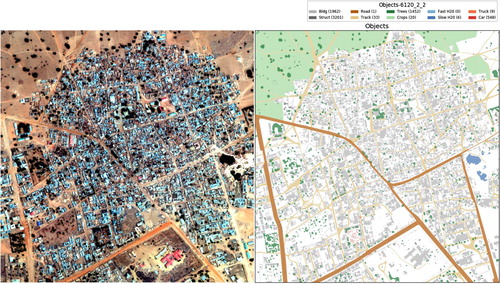
In a satellite image, there are lots of different objects like roads, buildings, vehicles, farms, trees, water ways, etc. DSTL has labelled 10 different classes: (1) Buildings – large building, residential, non-residential, fuel storage facility, fortified building; (2) Misc. Manmade structures; (3) Road; (4)Track – poor/dirt/cart track, footpath/trail; (5) Trees – woodland, hedgerows, groups of trees, standalone trees; (6) Crops - contour ploughing/cropland, grain (wheat) crops, row (potatoes, turnips) crops; (7) Waterway; (8) Standing water; (9) Vehicle Large – large vehicle (e.g. lorry, truck, bus), logistics vehicle; (10) Vehicle Small – small vehicle (car, van), motorbike. Figure 3 shows the distribution of each class in DSTL dataset. It is observed that the problem of class imbalance exists in this dataset. Figure 4 shows the original image and mask image of labelled objects in DSTL dataset.

Figure 3. Class distribution of DSTL dataset.

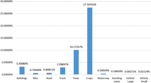
Figure 4. Labels of an image in DSTL dataset (left: original image; right: mask image of labeled objects).

4.3. Results

In the experiment we applied our approach to the DSTL dataset. The image patches are extracted with size 160 × 160 from the original images with flipped horizontally and vertically, and rotation. After data augmentation, the dataset is augmented by 14 times. We trained the modified U-Net model (Figure 2) for 100 epochs iterations on, with mini-batches of size 32. The parameters of Adam optimiser are ${\beta }_1=0.9$, ${\beta }_2=0.999$, $\epsilon ={10}^{-8}$ learning rate $\eta =0.001$. There are three metric functions for the model compiling: jaccard_coef (Jaccard index), jaccard_coef_int (Jaccard index with rounded predictive value) and accuracy. Figure 5 plots the evolution of metric functions through the iterations. The evaluation results of trained model are listed in Table 2. After 100 epochs training, the value of jaccard_similarity_score function in the scikit-learn library is 0.8752. We compared our approach with the FCN-based model without adaptive threshold to verify classification results for class imbalance. In addition, we also applied our approach to training dataset without data augmentation to validate the effectiveness of data augmentation, and compared our approach with patch-based CNN (proposed by Mnih V) (2013) and Binary logistic.

Figure 5. Performance evolution.

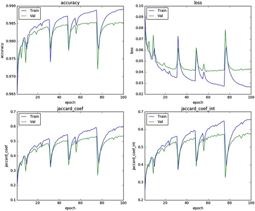
Table 2. Best threshold of each class.

Class	Buildings	Misc	Road	Track	Tree	Crops	Waterway	Standing water	Vehicle large	Vehicle small
Threshold	0.36	0.22	0.51	0.26	0.45	0.39	0.57	0.61	0.31	0.18

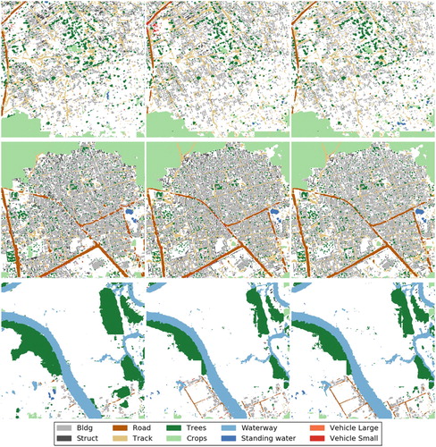
Figure 6 shows the prediction result of our method and visualises it as a group of mask images for every class. Figures 7 and 8 shows results of experiments compared with corresponding ground truth. It can be seen that the classification results are generally good for large objects such as buildings, road, trees and waterway. However, there are many erroneous results for the class of small objects which have not enough training data.

Figure 6. Mask images of a result predicted by our model.

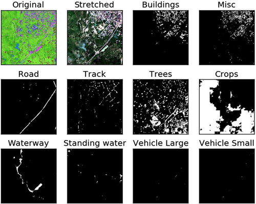
Figure 7. Experiments results on the DSTL dataset (from left to right: ground truth; results of our FCN-based model with adaptive threshold; results of our FCN-based model without adaptive threshold).

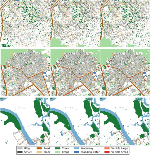
Figure 8. Experiments results on the DSTL dataset (from left to right: results of patch-based CNN model; results of our FCN-based model with adaptive threshold and without data augmentation; results of our FCN-based model without adaptive threshold and without data augmentation).

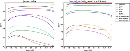
Adaptive threshold Jaccard similarity score was used to find the best threshold. Figure 9 shows the relationship between evaluation values of each class and thresholds. Table 2 shows the results of adaptive threshold. As shown in Figure 10, adaptive threshold significantly improves the segmentation performance of “vehicle small” class which has less training data than other classes. The results of our experiments can be seen in Table 3. From the table, it can be seen that the adaptive threshold algorithm can increase the score of average Jaccard index from 0.614 to 0.636 and increase the score of “Vehicle Small” class which has not enough training data from 0.166 to 0.238. Additionally, the proposed FCN model outperforms Binary logistic and patch-based CNN in terms of average Jaccard index. Data augmentation significantly improves the score of average Jaccard index. The experimental results prove that state-of-the-art performance on the remote sensing datasets is achieved with our approach. We argue that the effectiveness of the proposed approach comes from three reasons. Firstly, U-Net model simply concatenates the encoder feature maps to upsampled feature maps from the decoder at every stage to form a ladder like structure. Secondly, the architecture by its skip concatenation connections allows the decoder at each stage to learn back relevant features that are lost when pooled in the encoder. Finally, adaptive threshold algorithm adjusts threshold of each class to help model get better average Jaccard index.

Figure 9. The relationship between evaluation values and thresholds of two evaluation metrics (left: Jaccard Index; right: “jaccard_similarity_score” in the scikit-learn).

Figue 10. Experiments results of “vehicle small” class (from left to right: colour image; mask image of ground truth; mask image of our method; mask image of FCN without adaptive threshold).

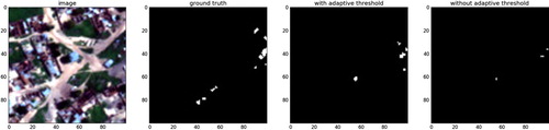
Table 3. Comparison among performances of the five methods.

Performance	Buildings	Misc	Road	Track	Tree	Crops	Waterway	Standing water	Vehicle large	Vehicle small	Average
Binary logistic	0.484	0.015	0.500	0.201	0.393	0.539	0.575	0	0	0	0.271
Patch-based CNN	0.623	0.146	0.756	0.258	0.671	0.958	0.873	0.800	0.001	0.030	0.512
FCN without adaptive threshold	0.698	0.152	0.863	0.455	0.728	0.969	0.917	0.830	0.359	0.166	0.614
Our method without data augmentation	0.599	0.138	0.568	0.219	0.451	0.878	0.829	0.707	0.042	0.047	0.448
Our method	0.705	0.258	0.864	0.472	0.728	0.969	0.919	0.835	0.369	0.238	0.636

5. Conclusion

This work addressed the problem of multiclass semantic segmentation for high-resolution remote sensing image with CNN. CNNs are mostly used to categorise images, semantic segmentation is an important method to implement object-oriented classification. Class imbalance is an important problem in remote sensing dataset. In this paper, we have applied an FCN-based model for dense pixel-wise classification in an end-to-end way. Adaptive threshold method is used to improve classification accuracy of classes that have not enough training data. The experimental results show that such networks outperform previous approaches in accuracy. It is proven that our approach has a strong applicability for the remote sensing image. The main limitation of our approach is the requirement of a large number of high-quality ground truth labels for the model training, which relies on professional interpretation experiences and lots of manual work. Therefore, the main aspect of our future work is training the model in a weak supervision way, to further enhance its applicability.

Disclosure statement

No potential conflict of interest was reported by the authors.

Additional information

Funding

This work was partially funded by the Ministry level fund No. 16A804 on developing the intelligence processing technique for remote sensing images.

References

- Amin, H. H., Deabes, W., & Bouazza, K. (2017). Clustering of user activities based on adaptive threshold spiking neural networks. Ninth international conference on ubiquitous and future networks, IEEE, Milan, Italy, 2017, 1–6.
- Atkinson, P. M., & Lewis, P. (2000). Geostatistical classification for remote sensing: An introduction. Computers & Geosciences, 26(4), 361–371.
- Badrinarayanan, V., Kendall, A., & Cipolla, R. (2017). Segnet: A deep convolutional encoder-decoder architecture for image segmentation. IEEE Transactions on Pattern Analysis and Machine Intelligence, 39(12), 2481–2495.
- Bischof, H., Schneider, W., & Pinz A, J. (1992). Multispectral classification of Landsat-images using neural networks. IEEE Transactions on Geoscience and Remote Sensing, 30(3), 482–490.
- Boureau, Y. L., Ponce, J., & LeCun, Y. (2010). A theoretical analysis of feature pooling in visual recognition. Proceedings of the 27th international conference on machine learning (ICML-10), 2010, 111–118.
- Chen, L. C., Papandreou, G., Kokkinos, I., Murphy, K, & Yuille, A.L. (2018). Deeplab: Semantic image segmentation with deep convolutional nets, atrous convolution, and fully connected crfs. IEEE Transactions on Pattern Analysis and Machine Intelligence, 40(4), 834–848.
- Cheng, G., & Han, J. (2016). A survey on object detection in optical remote sensing images. ISPRS Journal of Photogrammetry and Remote Sensing, 117, 11–28.
- Decatur, S. E. (1989). Application of neural networks to terrain classification. International joint conference on neural networks, IEEE, Vol. 1, 1989, 283–288.
- DSTL Satellite Imagery Feature Detection. (2017). Retrieved from https://www.kaggle.com/c/dstl-satellite-imagery-feature-detection
- Forestier, G., Puissant, A., Wemmert, C., & Gançarski, P. (2012). Knowledge-based region labeling for remote sensing image interpretation. Computers, Environment and Urban Systems, 36(5), 470–480.
- Fu, G., Liu, C., Zhou, R., Sun, T., & Zhang, Q. (2017). Classification for high resolution remote sensing imagery using a fully convolutional network. Remote Sensing, 9(6), 498.
- Garcia-Garcia, A., Orts-Escolano, S., Oprea, S., Villena-Martinez, V., & Garcia-Rodriguez, J. (2017). A review on deep learning techniques applied to semantic segmentation. Transactions on Pattern Analysis and Machine Intelligence, 0, 0. https://arxiv.org/abs/1704.06857
- Girshick, R., Donahue, J., Darrell, T., & Malik, J. (2014). Rich feature hierarchies for accurate object detection and semantic segmentation. Proceedings of the IEEE conference on computer vision and pattern recognition, Columbus, OH, 2014, 580–587.
- Han, J., Zhang, D., Cheng, G., Guo, L., & Ren, J. (2015). Object detection in optical remote sensing images based on weakly supervised learning and high-level feature learning. IEEE Transactions on Geoscience and Remote Sensing, 53(6), 3325–3337.
- Hentschel, C., Wiradarma, T. P., & Sack, H. (2016). Fine tuning CNNS with scarce training data – adapting imagenet to art epoch classification. IEEE international conference on image processing, IEEE, Phoenix, AZ, 2016, 3693–3697.
- Kaiser, P. (2016). Learning city structures from online maps. ETH Zurich, 2016.
- Kampffmeyer, M., Salberg, A. B., & Jenssen, R. (2016). Semantic segmentation of small objects and modeling of uncertainty in urban remote sensing images using deep convolutional neural networks. 2016 IEEE conference on computer vision and pattern recognition workshops (CVPRW), IEEE, Las Vegas, NV, 2016, 680–688.
- Kemker, R., & Kanan, C. (2017). Deep neural networks for semantic segmentation of multispectral remote sensing imagery. arXiv preprint arXiv, 1703.06452.
- Kingma, D. P., & Ba, J. (2014). Adam: A method for stochastic optimization. 3rd International Conference for Learning Representations, San Diego, 2015.
- Krizhevsky, A., Sutskever, I., & Hinton, G. E. (2012). Imagenet classification with deep convolutional neural networks. Advances in neural information processing systems. Proceedings of the 25th International Conference on Neural Information Processing Systems, 1, 1097–1105. Lake Tahoe, NV, December 3–6, 2012.
- Liu, Y., Minh Nguyen, D., Deligiannis, N., Ding, W., & Munteanu, A. (2017). Hourglass-shapenetwork based semantic segmentation for high resolution aerial imagery. Remote Sensing, 9(6), 522.
- Ma, A., Zhong, Y., & Zhang, L. (2015). Adaptive multiobjective memetic fuzzy clustering algorithm for remote sensing imagery. IEEE Transactions on Geoscience and Remote Sensing, 53(8), 4202–4217.
- Maggiori, E., Tarabalka, Y., Charpiat, G., & Alliez, P. (2016). Fully convolutional neural networks for remote sensing image classification. Geoscience and remote sensing symposium, IEEE, 2016, 5071–5074.
- Maggiori, E., Tarabalka, Y., Charpiat, G., & Alliez, P. (2017). Can semantic labeling methods generalize to any city? The INRIA aerial image labeling benchmark. IEEE international symposium on geoscience and Remote sensing (IGARSS), 2017.
- Marmanis, D., Datcu, M., Esch, T., & Stilla, U. (2016a). Deep learning earth observation classification using ImageNet pretrained networks. IEEE Geoscience and Remote Sensing Letters, 13(1), 105–109.
- Marmanis, D., Wegner, J. D., Galliani, S., et al. (2016b). Semantic segmentation of aerial images with an ensemble of CNNs. ISPRS Annals of the Photogrammetry, Remote Sensing and Spatial Information Sciences, 3, 473.
- Mnih, V. (2013). Machine learning for aerial image labeling. University of Toronto, Canada, 2013.
- Mountrakis, G., Im, J., & Ogole, C. (2011). Support vector machines in remote sensing: A review. ISPRS Journal of Photogrammetry and Remote Sensing, 66(3), 247–259.
- Muruganandham, S. (2016). Semantic segmentation of satellite images using deep learning. Lulea University of Technology, 2016.
- Noh, H., Hong, S., & Han, B. (2015). Learning deconvolution network for semantic segmentation. Proceedings of the IEEE international conference on computer vision, Santiago, Chile, 2015, 1520–1528.
- Pal, M. (2005). Random forest classifier for remote sensing classification. International Journal of Remote Sensing, 26(1), 217–222.
- Parvat, A., Chavan, J., Kadam, S., Dev, S., & Pathak, V. (2017). A survey of deep-learning frameworks. 2017 International conference on inventive systems and control (ICISC), IEEE, Coimbatore, India, 2017, 1–7.
- Penatti, O. A. B., Nogueira, K., & Santos, J. A. D. (2015). Do deep features generalize from everyday objects to remote sensing and aerial scenes domains? Computer vision and pattern recognition workshops, IEEE, Boston, MA, 2015, 44–51.
- Ronneberger, O., Fischer, P., & Brox, T. (2015). U-net: Convolutional networks for biomedical image segmentation. International conference on medical image computing and computer-assisted intervention, Springer, Cham, 2015, 234–241.
- Saito, S., Yamashita, T., & Aoki, Y. (2016). Multiple object extraction from aerial imagery with convolutional neural networks. Electronic Imaging, 60(1), 10402-1–10402-9.
- Semantic Labeling Contest[EB/OL]. (2018). Retrieved from http://www2.isprs.org/commissions/comm3/wg4/semantic-labeling.html
- Sharma, A., Liu, X., Yang, X., & Shi, D. (2017). A patch-based convolutional neural network for remote sensing image classification. Neural Networks, 95, 19–28.
- Shelhamer, E., Long, J., & Darrell, T. (2017). Fully convolutional networks for semantic segmentation. IEEE Transactions on Pattern Analysis and Machine Intelligence, 39(4), 640–651.
- Simonyan, K., & Zisserman, A. (2014). Very deep convolutional networks for large-scale image recognition. arXiv Preprint ArXiv, 1409.1556.
- Tuia, D., Moser, G., Le Saux, B., et al. (2017). IEEE GRSS data fusion contest: Open data for global multimodal land Use classification [technical committees]. IEEE Geoscience and Remote Sensing Magazine, 5(1), 70–73.
- Wei, Y., Wang, Z., & Xu, M. (2017). Road structure refined CNN for road extraction in aerial image. IEEE Geoscience & Remote Sensing Letters, 14(5), 709–713.
- Zhang, L., Zhang, L., & Du, B. (2016). Deep learning for remote sensing data: A technical tutorial on the state of the art. IEEE Geoscience and Remote Sensing Magazine, 4(2), 22–40.
- Zhao, B., Feng, J., Wu, X., & Yan, S. (2017). A survey on deep learning-based fine-grained object classification and semantic segmentation. International Journal of Automation and Computing, 14(2), 119–135.
- Zhong, Y., Fei, F., Liu, Y., et al. (2017). SatCNN: Satellite image dataset classification using agile convolutional neural networks. Remote Sensing Letters, 8(2), 136–145.