Learning adversarial policy in multiple scenes environment via multi-agent reinforcement learning

ABSTRACT

Learning adversarial policy aims to learn behavioural strategies for agents with different goals, is one of the most significant tasks in multi-agent systems. Multi-agent reinforcement learning (MARL), as a state-of-the-art learning-based model, employs centralised or decentralised control methods to learn behavioural strategies by interacting with environments. It suffers from instability and slowness in the training process. Considering that parallel simulation or computation is an effective way to improve training performance, we propose a novel MARL method called Multiple scenes multi-agent proximal Policy Optimisation (MPO) in this paper. In MPO, we first simulate multiple parallel scenes in the training environment. Multiple policies control different agents in the same scene, and each policy also controls several identical agents from multiple scenes. Then, we expand proximal policy optimisation (PPO) with an improved actor-critic network, ensuring the stability of training in multi-agent tasks. The actor network only uses local information for decision making, and the critic network uses global information for training. Finally, effective training trajectories are computed with two criteria from multiple parallel scenes rather than single to accelerate the learning process. We evaluate our approach in two simulated 3D environments, one of which is Unity's official open-source soccer game, and the other is unmanned surface vehicles (USVs) built by Unity. Experiments demonstrate that MPO converges more stable and faster than benchmark methods in model training, and demonstrates excellent adversarial policy compared with benchmark models.

Keywords:

• Adversarial policy
• multiple scenes
• multi-agent systems
• multi-agent reinforcement learning
• proximal policy optimisation

1. Introduction

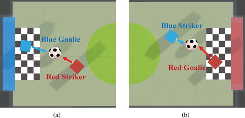
Considering many applications of multi-agent system, such as multiplayer games (Hernandez-Leal et al., 2014; Peng et al., 2017), Poker games (Billings et al., 1998), USVs combat training (Raboin et al., 2015), network packet routing (Tao et al., 2001), robots control (Barakova et al., 2018; Matignon et al., 2012), traffic agents control (Bacchiani et al., 2019; Brys et al., 2014; Yu et al., 2019) and so on, most of the applications contain elements of adversary and conflict. Learning adversarial policy for agents in multi-agent applications becomes more important and has recently attracted much interest in the research community. Unlike learning cooperative policy for all agents to maximise a team goal, learning adversarial policy needs to model behavioural strategy for different agents in the same scene and pursue their own goals. Figure 1 shows a representative example: soccer game. Figure 1(a) demonstrates that blue goalie needs to prevent soccer from being scored by red striker. Blue striker tries to kick soccer to the goal, which is prevented by red goalie (Figure 1 b). The soccer game scene illustrates the adversarial relationship between goalies and strikers. Adversarial policy learning methods should be able to model the policies of goalies and strikers, and optimise the policies so that both opponents can maximise their goals.

Figure 1. The adversarial relationship between goalies and strikers in soccer game scene.

A conventional approach to learning adversarial policy is to formulate it as an optimisation problem (Dineva & Schöner, 2018; Kheyrinataj & Nazemi, 2020; Nazemi et al., 2019) with agent dynamics and multi-agent environment models. Most of traditional works are based on understanding agent dynamics and the information of multi-agent environments, including position, velocity and goal location of all agents. The game theory-based methods (Singh et al., 2000; Zhang & Lesser, 2010) formulate the problem as an optimisation problem, and the goal is to make agent's behavioural policy converge to Nash equilibrium (Nash, 1950) with multi-agent learning criteria, which assumes that an agent should be able to converge to a stationary policy against some opponents and the best response policy against any stationary opponent. However, it is not easy to accurately derive the dynamics of agents in many applications, because some parts of complex multi-agent system are hard to model. Also, they need opponents to remain stationary for a long enough period to learn policy (Hernandez-Leal et al., 2017), which can be unrealistic in dynamically changing environments. Multi-agent reinforcement learning (MARL), as a state-of-the-art learning-based model, has shown great success recently in multi-agent policy learning tasks (Jaderberg et al., 2019; Semnani et al., 2020; Wang et al., 2020). Instead of relying on the understanding of system and the explicit motion equations of agents to design models, MARL allows agents to learn strategies by interacting with environment.

Concerning multi-agent policy learning tasks, MARL mainly adopts two categories: centralised and decentralised approaches. The centralised approaches focus on using central policy to generate global control actions based on global observations of all agents (Movric & Lewis, 2013; Wang et al., 2020). However, the centralised MARL methods rely on global observations makes it challenging to deploy in practice because, in the process of learning adversarial policy, agent can only make decisions based on local observation. Unlike the centralised methods, many MARL approaches have focused on entirely decentralised policies. Each agent selects actions independently of all other agents using its observations (Jaderberg et al., 2019; Long et al., 2018; Semnani et al., 2020). Compared with centralised approaches, decentralised policies have the advantages of scalability and parallelisability. The decentralised methods allow different agents to pursue different objectives, which causes non-stationary problem and often leads to unstable learning or the convergence to poorly performing policies. Some methods solve the above problem with the framework of centralised training with decentralised execution (Liu et al., 2020; Lowe et al., 2017; Mao et al., 2019; Ryu et al., 2020). During centralised training, methods utilise global information, and agents take actions based on local during decentralised execution. Although the above methods can alleviate the instability of training, they still suffer from slowness during training due to the shortage of effective training data. Some papers (Barrett et al., 2014; Mnih et al., 2016; Sartoretti et al., 2019) use distribute learning method in single-agent problems to collect effective training data from multiple simulators. The purpose of these methods is to ensure the stability of learning, accelerate training and ultimately improve policies' performance. However, the global policy network used in the above methods cannot be transferred to learn adversarial policy directly because of agents' different objectives under adversarial setting.

In this paper, inspired by distribute learning methods (Mnih et al., 2016; Sartoretti et al., 2019), we propose a novel MARL method to ensure the stability of learning and accelerate training process. The method called Multiple Scenes Multi-Agent Proximal Policy Optimisation, is based on actor-critic network. In our approach, we first simulate multiple scenes with different initial position settings for agents. Each policy controls several identical agents from different scenes and can interact with multiple scenes simultaneously. We then use multiple improved actor-critic networks as policy models with different initial weights to control different agents in single scene. The actor networks only use local observation as input for decision making, and the critic networks use the observations of all agents for model training. Such network design has been shown to improve MARL performance significantly (Lowe et al., 2017). Finally, we propose two criteria to compute effective training trajectories after all trajectories from multiple parallel scenes are gathered. In our experiments, we evaluate the performance of our algorithm with PPO (Schulman et al., 2017) and MADDPG (Lowe et al., 2017) on two multi-agent simulated 3D environments, which shows excellent adversarial policy and short training time of our proposed approach.

The main contributions of our proposed approach are the following:

• We propose a novel MARL method with improved actor-critic network, which provides good performance in adversarial policy learning tasks.

• We collect effective training trajectories from multiple parallel scenes in the training environment to make our approach converges fast to the global minimum.

• We evaluate the proposed method on multi-agent adversarial environments and show its better performance than state-of-the-art baselines.

The rest of this paper is organised as follows. In Section 2, we present some related work about multi-agent reinforcement learning. Section 3 introduces reinforcement learning (RL) background in multi-agent domains. Section 4 describes our multiple scenes multi-agent proximal policy optimisation method. Section 5 introduces the experimental environments, which include USVs and soccer environments. In Section 6, we present and analyse experimental results. Finally, we conclude this paper and discuss some directions for future work in Section 7.

2. Related work

This section reviews the current related work on multi-agent reinforcement learning. In conjunction with the needs in adversarial strategy modelling, multi-agent reinforcement learning methods can be divided into three main categories, including multi-agent reinforcement learning with centralised learning, multi-agent reinforcement learning with decentralised learning, and multi-agent reinforcement learning with distributed learning. The adversarial strategy modelling method proposed in this paper belongs to both decentralised learning and distributed learning. It comprehensively uses and improves the single-agent reinforcement learning algorithm, adopts decentralised learning for multi-agent adversarial strategy modelling and uses a multi-scene distributed learning approach for model training, which significantly improves the model performance and learning speed.

2.1. MARL with centralised learning

Several recent studies are looking to multi-agent reinforcement learning approaches for multi-agent policy learning problems. MARL methods offload the expensive real-time policy computations to an off-line training procedure (Foerster et al., 2018; Long et al., 2018; Lowe et al., 2017; Matignon et al., 2012; Semnani et al., 2020). The straightforward approach is to use a centralised learning method. Long et al. propose a sensor-level collision avoidance strategy for multi-robot systems. Semnani et al. solve distributed multi-agent motion planning problem in dense and dynamic environments with improved centralised learning MARL approach. Some methods with optimistic and hysteretic Q function updates (Lauer & Riedmiller, 2000; Matignon et al., 2007; Omidshafiei et al., 2017) use all agents' actions to improve global reward. Gupta et al. share policy parameters between agents via integrating the capability of agents (Gupta et al., 2017). However, the global reward function of centralised learning method is not suitable in multi-agent adversarial environment since different kinds of agents have different reward functions.

2.2. MARL with decentralised learning

In contrast to centralised approaches, decentralised methods are more suitable for adversarial policy learning problem. Independent Q-learning method (Matignon et al., 2012) with decentralised learning has been used for multi-agent policy learning, which is based on Q-learning (Watkins & Dayan, 1992). Long et al. present a decentralised approach based on MARL for multi-robot collision avoidance (Long et al., 2018). Semnani et al. solve the multi-agent motion planning problem with a MARL-based decentralised method (Semnani et al., 2020). Although decentralised methods are appropriately scalable as they distribute the computational effort over multiple agents, they still face many challenges. The main reason why decentralised formulations have poor performance is that the environment becomes non-stationary because each agent's policy changes when training. It does not meet the Markov assumption of Markov decision process, which is an essential assumption of most reinforcement learning methods. Some previous works (Foerster et al., 2017; Tesauro, 2004) combine the policy parameters of other agents with Q function to solve this problem, but could not solve the problem well. The framework of centralised training with decentralised execution has been proposed to solve non-stationary problem (Foerster et al., 2018; Lowe et al., 2017; Mao et al., 2019). In this framework, each agent relies on independent actors to make decisions and estimates policy evaluation via a central critic, which takes global information generated by agents as input. Foerster et al. used policy gradient methods with a centralised critic, and they trained a single centralised critic for all agents in multi-agent scenes (Foerster et al., 2018). On StarCraft tasks, their method has excellent performance.

2.3. MARL with distributed learning

Although decentralised methods can apply to multi-agent adversarial learning, they still require sizeable effective training data to train model. In terms of speeding up training process, asynchronous advantage actor-critic (A3C) (Mnih et al., 2016) train policy with distributed scenes. Multiple agents act in their copy of scenes simultaneously. The gradients are calculated separately and sent to a central parameter policy that asynchronously updates a central copy of the model. Based on A3C, Sartoretti et al. present a distributed learning method that learns multi-agent control policies (Sartoretti et al., 2019). Their method also needs a global policy network to control the update of policies for multiple agents.

Similar to our approach, methods in Lowe et al. (2017) and Mao et al. (2019) solve multi-agent policy learning tasks based on the framework of centralised training with decentralised execution. Although the methods use feed-forward policies and learn centralised critic for each agent, it does not consider how to choose effective trajectories to reduce training time. In contrast to the distributed methods in Mnih et al. (2016) and Sartoretti et al. (2019), because of the different reward functions of each agent in adversarial scene, we do not set a global policy network for all agents.

3. Preliminaries

3.1. Markov decision processes

The method we propose is based on reinforcement learning. RL is modelled according to Markov Decision Processes, which is mainly composed of a five-tuple $<S,A,r,T,{\rho }_0>$, where S and A denote the set of state and action, $r:S\times A\to R$ denotes a reward function. When an agent takes an action $A_0$ in a state $S_0$, it will receive a reward $r_0$ from environment. $T:S\times A\to \mathrm{\Delta }\left(S\right)$ denotes a transition function, where $\mathrm{\Delta }\left(S\right)$ is the set of discrete probability distributions over S. ${\rho }_0\to [0,1]$ denotes initial state distribution. The agent in the environment learns a stochastic policy $\pi :S\times A\to [0,1]$ to maximising the discounted expected future reward: $E_{\pi }\left[\sum _{t=0}^{\mathrm{\infty }}{\gamma }^{t}r\right(s_t{a}_t\left)\right]$, where $\gamma \in [0,1]$ is a discount factor and t is the time step.

3.2. Markov games

We model learning adversarial policy with MARL as partially observable Markov game. The Markov game is a multi-agent extension of Markov decision processes (MDPs) (Hu & Wellman, 1998; Littman, 1994). A partially observable Markov game for N agents consists of a set of states S, actions $a^{\left(1\right)},\dots ,a^{\left(i\right)},\dots ,a^{\left(N\right)}$ and observations $O^{\left(1\right)},\dots ,O^{\left(i\right)},\dots ,O^{\left(N\right)}$ for each agent. Each agent i takes actions through a stochastic policy π, and the next state $S^{\mathrm{\prime }}$ is generated by the state transition function $Tran:S\times a^{\left(1\right)}\times \cdots a^{\left(i\right)}\cdots \times a^{\left(N\right)}\to S^{\mathrm{\prime }}$. The reward function $r^{\left(i\right)}:S\times a^{\left(i\right)}\to R$ indicates relationship between the state and action of each agent i, R is a set of real numbers. Each agent i aims to maximise its own discounted sum of future rewards $R^{\left(i\right)}=\sum _{t=0}^T{\gamma }^t{r}_t^{\left(i\right)}$ where γ denotes a discount factor and T denotes the time horizon.

3.3. Policy gradient methods

Policy gradient methods are realised by combining policy gradient and stochastic gradient ascent algorithms, which have been used for many tasks. The gradient of the policy can be written as (1) ${\mathrm{\nabla }}_{\theta }J\left(\theta \right)={\mathbb{E}}_{s\sim p^{\pi },a\sim {\pi }_{\theta }}[{\mathrm{\nabla }}_{\theta }\log {\pi }_{\theta }(a|s\left)Q^{\pi }\right(s,a\left)\right],$(1) where $p^{\pi }$ denotes the state distribution. The improved algorithms of policy gradient method differ primarily in the way of estimating $Q^{\pi }$. Some methods learn an approximation of true action-value function $Q^{\pi }(s,a)$ such as temporal-difference learning (Sutton & Barto, 2018). Some methods simply use a sample return $R^t=\sum _{i=t}^T{\gamma }^{i-t}{r}_i$, such as the REINFORCE algorithm (Williams, 1992). $Q^{\pi }(s,a)$ is often called as the critic and a variety of actor-critic algorithms (Sutton & Barto, 2018) are proposed.

3.4. Proximal policy optimisation

Different from existing MARL method, we extend Proximal Policy Optimisation (PPO) (Schulman et al., 2017) to multi-agent field. PPO belongs to the policy gradient algorithm of single reinforcement learning. It uses a stochastic gradient ascent to optimise surrogate objective function and alternates sampled data by interacting with scene. Unlike standard policy gradient method, PPO does not perform a gradient update on each data sample but utilises small batch updates. It not only makes the sample more complicated but also makes the algorithm easier to implement. It roughly clip the ratio between ${\pi }_{\theta }$ and ${\pi }_{{\theta }_{old}}$ and change the surrogate objective function into the form (2) $\begin{array}{rl}{L}^{clip}\left(\theta \right)& =\mathbb{E}[min(ratio\left(\theta \right)adv,\\ & clip\left(ratio\right(\theta ),1-ϵ,1+ϵ)adv\left)\right],\end{array}$(2) where adv is an estimator of the advantage function, $ratio\left(\theta \right)={\pi }_{\theta }/{\pi }_{{\theta }_{old}}$ denotes the probability ratio, θ is the parameter of π and ϵ is a hyper parameter.

4. Multiple scenes multi-agent proximal policy optimisation

Considering that parallel simulation or computation is an effective way to reduce current learning cost, we propose multiple scenes multi-agent proximal policy optimisation, a multi-agent reinforcement learning method. The originality of method is based on the assumption that the training environment can run several scenes in parallel. The usage of method is confined to the training phase. In this section, we mainly introduce the method from three aspects below.

4.1. Multiple scenes environment

As shown in Figures 4(a) and 5(a), the training environment contains multiple scenes. Each scene has the same settings, including the type and number of agents. Each scene has an interface to interact with adversarial policy model, including scene initialisation, state information acquisition, action execution and reward calculation. Adversarial Policy models can interact with multiple scenes simultaneously at training time. Each type of agents in different scenes shares an actor-critic network, but the initial state of each agent in every scene may be different. In detail, if there are N kinds of agents in each scene and a total of M scenes, there will be N actor-critic networks, and each network corresponds to a type of agent. As shown in Figure 2, at time step t, the observation of ith kind of agent is $O_t^{\left(i\right)}=(O_t^{\left(i1\right)},O_t^{\left(i2\right)},\dots ,O_t^{\left(ij\right)}\cdots ,O_t^{\left(iM\right)}),j\in 1,\dots ,M$. The state of environment S at t is $S_t=(O_t^{\left(1\right)},O_t^{\left(2\right)},\dots ,O_t^{\left(i\right)},\dots ,O_t^{\left(N\right)})$. Actor network accepts $O_t^{\left(i\right)}$ as input at time t and outputs the actions of ith kind of agent in each scene. Distributed learning in a multiple scenes environment does not require an additional increase in the number of adversarial models. The same model controls different types of agents in each scene. Since scenes are run simultaneously, the adversarial policy model can obtain training data from M scenes at the same time. Compared with existing distributed learning methods (Mnih et al., 2016; Sartoretti et al., 2019), our approach is more suitable for scenes with multiple agents of various types because there is no need to set up a global model while obtaining a large amount of training data.

Figure 2. The framework of multiple scenes multi-agent proximal policy optimisation.

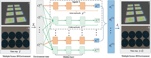
Figure 3. Illustration of the adversarial policy learning process of our method.

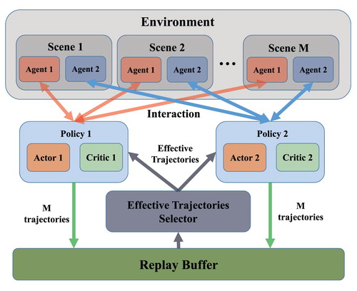
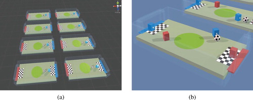
Figure 4. The specific scenarios in our experimental environment: (a) the global perspective of environment, (b) some specific details, (c) and (d) the perspective of attacker and defender.

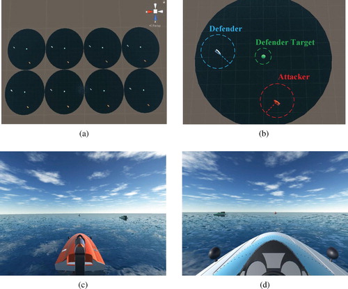
Figure 5. The soccer environment based on Unity platform: (a) a global perspective of entire environment which contains multiple trainable scenes and (b) the first perspective of each scene during training.

4.2. Adversarial policy modelling

Because of each agent's different reward function, we set multiple networks as policy models with different initial weights to control agents. As shown in Figure 2, our approach is based on actor-critic network. The policy model of each agent consists of an actor network and a critic network. Furthermore, actor network π and critic network V all have three hidden layers. The actor network output actions and the critic network with the observations of all agents are used to training the entire model. At time step t, policy model get environment state $S_t$ which contains observations of agents in multiple scenes 3D environment and output joint action $A_t$. Actor networks only use the local observation of ith kind of agent as input, and global critic networks use the observations of all agents. Based on that, we apply PPO with the framework of centralised training with decentralised execution to ensure the stability of learning process. Considering a scene with N kinds of agents with actors parameterised by $\theta =\{{\theta }^{\left(1\right)},\dots ,{\theta }^{\left(N\right)}\}$, $\pi =\{{\pi }^{\left(1\right)},\dots ,{\pi }^{\left(N\right)}\}$ is the set of all agent actors in a scene, $V=\{V^{\left(1\right)},\dots ,V^{\left(N\right)}\}$ is the set of all agent critics, $\varphi =\{{\varphi }^{\left(1\right)},\dots ,{\varphi }^{\left(N\right)}\}$ is critics parameterised. Each agent takes action through its own observations and learns critic through the observations of all agents. We denote the action of ith agent at time step t as $a_t^{\left(i\right)}$. The actions of all agents in environment $A_t=(a_t^{\left(1\right)},\dots ,a_t^{\left(N\right)})$. The actor ${\pi }^{\left(i\right)}$ accepts $O_t^{\left(i\right)}$ as input at time t: (3) $a_t^{\left(i\right)}={\pi }_{{\theta }^{\left(i\right)}}^{\left(i\right)}\left(O_t^{\left(i\right)}\right),$(3) and the critic $V^{\left(i\right)}$ accepts the observations of all agents $(O_t^{\left(i\right)},O_t^{-})$: (4) $V_t^{\left(i\right)}=V_{{\varphi }^{\left(i\right)}}^{\left(i\right)}\left(\right(O_t^{\left(i\right)},O_t^{-}\left)\right),$(4) where $O_t^{-}$ denotes the observation of other agents at time step t. The critic $V^{\left(i\right)}$ outputs the value of the current state S to ith agent.

4.3. Policy learning with multiple scenes

To illustrate specific adversarial policy learning process, we consider a two-agent system as a concrete example of MPO. Figure 3 shows how decisions and training data flow. There are two agents in a single scene which have different reward function. According to the above subsection, two policies control two agents in each scene, respectively. Each policy interacts with a training environment containing multiple scenes and trains actor-critic network with effective trajectories from replay buffer. The process can be divided into two parts. In the first part, each actor ${\pi }^{\left(i\right)}$ controls a group of M agents in M scenes, and these agents are running in parallel, where i represents the set of related policy serial numbers. Actor ${\pi }^{\left(i\right)}$ outputs actions according to Equation (3(3) $a_t^{\left(i\right)}={\pi }_{{\theta }^{\left(i\right)}}^{\left(i\right)}\left(O_t^{\left(i\right)}\right),$(3) ) with observation $O^{\left(i\right)}$ and receives reward r from environment. When all agents have finished a complete episode, M trajectories of each policy are stored in the replay buffer. This part permits collect training trajectories into a global replay buffer.

Policies update is then performed in the second part with effective trajectories selected by effective trajectories selector from global replay buffer. Each policy is going to be fed with effective trajectories from agents that it controls and a bunch of ones from agents controlled by other policies at time t. Based on our previous work (Zhang et al., 2019), we define two sorts of effective trajectories. (1) Complete trajectories, where an agent successfully achieves the final goal. (2) Auxiliary trajectories, where an agent does not achieve the final goal but gets a higher cumulative return. We select complete trajectories and auxiliary trajectories for each policy from global replay buffer. Each policy computes gradient with effective trajectories to update actor-critic networks, accelerating and stabilising the training process.

In practice, if ${\pi }_{{\theta }_{old}}$ is too small that exceeds the floating range of computer, the denominator of ratio $ratio\left(\theta \right)={\pi }_{\theta }/{\pi }_{{\theta }_{old}}$ in Equation (2(2) $\begin{array}{rl}{L}^{clip}\left(\theta \right)& =\mathbb{E}[min(ratio\left(\theta \right)adv,\\ & clip\left(ratio\right(\theta ),1-ϵ,1+ϵ)adv\left)\right],\end{array}$(2) ) is approximately zero. The above problem may lead to the gradient of model not being calculated correctly when using deep learning framework, e.g. TensorFlow. In our experiments, unlike standard PPO, we change ratio from fractional to subtraction. The update of new policy is limited to the range of $[-ϵ,ϵ]$. Based on that, the objective function of the ith policy's actor network can be written as (5) $L^{clip}\left({\theta }^{\left(i\right)}\right)={\mathbb{E}}_t[min(rati{o}_t\left({\theta }^{\left(i\right)}\right)ad{v}_t^{\left(i\right)},clip\left(rati{o}_t\right({\theta }^{\left(i\right)}),-ϵ,ϵ)ad{v}_t^{\left(i\right)}\left)\right],$(5) where $rati{o}_t\left({\theta }^{\left(i\right)}\right)={\pi }_{{\theta }^{\left(i\right)}}\left(a_t^{\left(i\right)}|O_t^{\left(i\right)}\right)-{\pi }_{{\theta }_{old}^{\left(i\right)}}(a_t^{\left(i\right)}|O_t^{\left(i\right)}$, ϵ is a hyper parameter, and the advantage $ad{v}_t^{\left(i\right)}$ is defined as (6) $ad{v}_t^{\left(i\right)}=-V(O_t^{\left(i\right)},O_t^{-})+r_t^{\left(i\right)}+\gamma r_{t+1}^{\left(i\right)}+\cdots +{\gamma }^{T-t+1}{r}_{T-1}^{\left(i\right)}+{\gamma }^{T-t}V(O_T^{\left(i\right)},O_T^{-}),$(6) where t specifies the time index in $[0,T]$. 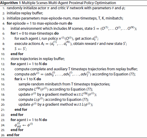The loss function of its critic network can be written as (7) $L\left({\varphi }^{\left(i\right)}\right)=-{\left(\sum _{t^{\mathrm{\prime }}>t}{\gamma }^{t^{\mathrm{\prime }}-t}{r}_{t^{\mathrm{\prime }}}^{\left(i\right)}-V_{{\varphi }^{\left(i\right)}}(O_t^{\left(i\right)},O_t^{-})\right)}^2.$(7) A detailed description of our method is presented in Algorithm 1.

5. Experiment environment construction

In this section, we introduce two training environments based on Unity platform, one of which is the soccer environment provided by Unity, and the other is the USVs environment built by some of the existing components in Unity, such as water, ship component. ¹

5.1. Unity platform for MARL

At present, many simulation platforms can provide a reinforcement learning environment, such as OpenAI Gym (Brockman et al., 2016), which can directly verify the feasibility and performance of algorithms by interacting with environments. However, these simulation platforms are black boxes for users because most of these platforms are not modifiable and lack flexibly configurable. The Unity platform has been widely used as a 3D environment modelling tool and game development engine. The platform's developers provide Unity Machine Learning Agents Toolkit (ML-Agents Toolkit) (Juliani et al., 2018), which is an open-source Unity plugin that allows users to develop their games or simulation scenarios as a training environment for reinforcement learning agents. At the same time, ML-Agents Toolkit also supports multi-agent environments. Developers can use their reinforcement learning algorithms and train agents through Python API, which helps the research of our multi-agent algorithms.

5.2. Unmanned surface vessels environment

We use the Unity introduced in the previous section to create Unmanned Surface Vessels (USVs) Environment. As shown in Figure 4, the environment includes one guard target area and two USVs, which are controlled by our algorithm. Of two USVs with mobility, one is defender and the other is attacker. The defender needs to hunt down attacker in time and ensures that the guard target area is not impacted. The attacker needs to get rid of defender and reach the guard target area. At the same time, neither defender nor attacker can leave the training area we set. In the process of building environment, we use physics engine in Unity to simulate the rigid body dynamics of USV, and we also simulate the resistance and buoyancy of water to USV. We use the USVs environment as a validation environment for our algorithm to verify algorithm's feasibility in multiple USV domains.

Since two USVs only have local observations in our environment, USV can obtain its position and velocity information. If enemy USV enters observation range, then his position and speed information will also be obtained. The observation of each agent in environment is a vector with a dimension of 12. Besides, due to the special nature of USV dynamics model, the USV cannot brake and reverse like a vehicle. It only has two action outputs: accelerator and rudder angle.

In our experiment's adversarial environment, it is not suitable for two USVs to share a reward function. So we set different reward functions for two USVs. For attacker, its reward value is inversely proportional to the distance from guard target and is proportional to the distance from guard target area. For defender, its reward value is inversely proportional to the distance from attacker and is proportional to the distance from guard target area. If defender insists on the end of episode, which contains 1000 steps, defender wins and receives a fixed bonus. If attacker reaches the area where target defended, attacker wins and receives a fixed reward.

5.3. Soccer environment

Unity officially provides a soccer environment for multi-agent learning algorithms. As shown in Figure 5, the environment contains multiple soccer game scenes, each scene consists of two teams and each team contains a goalie and a striker. The observation of each agent is a vector of dimension 112, including the position and speed of teammates and opponents. Goalie can perform five actions, and striker can perform seven actions. Goalie and striker are in an adversarial relationship, goalie needs to prevent soccer from entering goal area, and striker needs to kick soccer into goal. In training, our algorithm controls goalie and striker in the scene separately. If soccer enters goal area, goalie will be punished, and striker will be rewarded.

To evaluate the feasibility of our proposed algorithm and its superiority over other algorithms, we need a widely used environment to train our algorithm. As an authoritative machine learning training environment provided by Unity, the soccer environment is convincing. The application of many classical algorithms verifies the training of environment. It can provide an opportunity to compare our algorithms with other algorithms fairly.

6. Experimental results

In this section, based on the ML-Agents Toolkit, we first evaluate our method in the two Unity-based learning environments described in Section 5. We compare MPO with PPO and MADDPG, and show the quantitative and qualitative results of training process. For the different characteristics of USVs and soccer environment, we set different parameters for MPO, PPO and MADDPG. The relevant hyper-parameter settings of the above methods are shown in Table 1. Besides, for performance comparison between our approach and other methods, we conduct additional experiments to test the performance of our trained model through Success Rate, which indicates the number of times agent completed tasks in 1000 test experiments.

Table 1. Hyper-parameter settings in USVs and soccer environment.

	USVs environment			Soccer environment
Hyper-parameter	MPO	PPO	MADDPG	MPO	PPO	MADDPG
Batch size	1024	1024	1024	128	128	128
Buffer size	20,480	20,480	20,480	2000	2000	2000
Gamma	0.99	0.99	0.95	0.99	0.99	0.95
Lambda	0.95	0.95	–	0.95	0.95	–
Max steps	20,000,000	20,000,000	20,000,000	500,000	500,000	500,000
Layers	3	3	3	3	3	3
Beta	0.005	0.005	–	0.01	0.01	–
Epsilon	0.2	0.2	–	0.2	0.2	–
Hidden units	256	256	256	128	128	128
Learning rate	0.003	0.003	0.003	0.001	0.001	0.001
Epoch	3	3	–	3	3	–
Tau	–	–	0.01	–	–	0.01

6.1. Comparison in model training process

In the USVs and soccer environment, the number of scenes M is set to 2. We used MPO, PPO and MADDPG to control agents, and trained all models for 20,000 and 500 episodes in each training environment separately. Figures 6 and 7 show their learning curves in terms of mean reward. For all models, the shadowed area is enclosed by the min and max values of three training runs, and the solid lines in middle are mean value (same for Figures 8 and 9).

Figure 6. The mean episode rewards of MPO, PPO and MADDPG in the USVs environments: (a) MPO vs. PPO and (b) MPO vs. MADDPG.

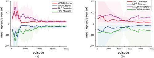
Figure 7. The mean episode rewards of MPO, PPO and MADDPG in the soccer environments: (a) MPO vs. PPO and (b) MPO vs. MADDPG.

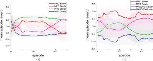
Figure 8. The figure shows the learning curve compares MPO results in three USVs environments, with different scenes number M: (a) one scene vs. two scenes, (b) two scenes vs. four scenes. (a) $M=1$ vs. M = 2. (b) M = 2 vs. M = 4.

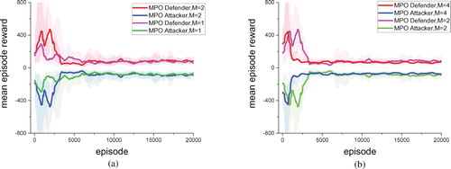
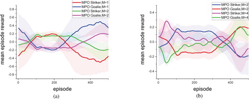
Figure 9. The figure shows the learning curve compares results of MPO in four soccer environments, which with different scenes number M: (a) one scene vs. two scenes, (b) two scenes vs. four scenes. (a) M = 1 vs. M = 2. (b) M = 2 vs. M = 4.

In each episode, if an agent receives a positive reward, adversarial agent gets a negative reward, so the reward learning curve of two agents is symmetrical about the episode coordinate axis. During training, the learning curves of two competitors will gradually approach each other until the model is trained to converge, which also means that the decision models of both parties are trained to the best. Therefore, comparing the performance of two methods is to see which learning curve can converge first. As observed in experiment results, MPO converges faster in USVs and soccer environments than other baselines, and its learning curve is more stable than PPO and MADDPG. The result shows that the effective trajectories selector in MPO makes training process more efficiently than PPO and MADDPG.

We compared the learning curve of MPO under different scenes numbers to evaluate the impact of multiple parallel scenes on MPO training. In the USVs environment, we construct three environments with a different number of scenes, and the number M is 1, 2, 4. We used MPO to control agents and trained all models for 20,000 episodes in each training environment separately. Figure 8 shows their learning curves in terms of mean reward. In the soccer environment, we also construct three environments with a different number of scenes, and the number M is 1, 2, 4. We trained MPO in each environment for 500 episodes and compare the mean episode reward learning curves of models in different environments, as shown in Figure 9. By evaluating MPO's performance in an environment containing a different number of scenes, MPO's learning speed increases with the number of scenes, whether it is USVs or soccer environment. The result indicates that the number of scenes M in training process has a positive impact on model's convergence speed. The larger M, the more Markov sequences can be obtained at each moment. This means that policy model can use more data for learning and significantly improve model's learning speed.

6.2. Performance of trained models

We compare the performance of MPO with two other models PPO and MADDPG. First, each model is trained with self-playing (i.e. Defender and Attacker are trained with same model in USVs environment). Then, in the same environment, the trained strategy and other strategies trained by different models control different agents, respectively. Finally, two indicators of Success Rate and trajectory are used to evaluate the performance of model. Tables 2 and 3 summarise the Success Rate indicates the probability that agent completes tasks in 1000 test experiments. The attacker's task in USVs environment is to reach target area without being captured by defender. Moreover, the task of striker in soccer environment is to kick soccer into goal. As shown in tables, the attacker trained by MPO has a higher Success Rate than PPO and MADDPG when competing with defender trained by other models. Similarly, the striker trained by MPO has higher Success Rate than PPO and MADDPG when competing with goalie trained by different models.

Table 2. The Success Rate for attacker in USVs environment.

USVs environment	Defender
Attacker	PPO	MADDPG	MPO (Ours)
PPO	49.3%	40.7%	20.8%
MADDPG	61.9%	52.1%	40.2%
MPO (Ours)	80.6%	72.3%	53.5%

Table 3. The Success Rate for striker in soccer environment.

Soccer environment	Goalie
Striker	PPO	MADDPG	MPO (Ours)
PPO	47.1%	39.3%	22.6%
MADDPG	65.5%	51.7%	38.2%
MPO (Ours)	81.3%	76.4%	50.9%

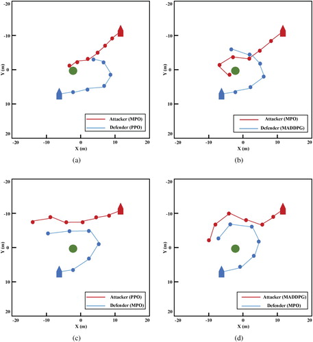
Figure 10 illustrates the trajectory of PPO, MADDPG and MPO in USVs environment. Trajectories are represented by red and blue lines. Red and blue circles represent the positions of attacker and defender at six-time steps. The green circle represents target area. From Figure 10(a,b), it can be seen that the attacker controlled by MPO can reach target area with the fastest trajectory while avoiding being intercepted by defenders controlled by PPO and MADDPG. It can also be seen from Figure 10(c,d) that the defender can intercept attackers controlled by PPO and MADDPG in time using the MPO model. These behaviours indicate that MPO learned an adversarial joint policy and has better performance than baseline approaches. Our policy produces more adversarial behaviour and efficient trajectory comparing to PPO and MADDPG.

Figure 10. The figure illustrates the trajectories of PPO, MADDPG and MPO under USVs environment.

7. Conclusion and future work

In this paper, we presented multiple scenes multi-agent adversarial policy learning method for addressing the current shortcomings in existing approaches to MARL and demonstrated its effectiveness on two multi-agent adversarial tasks. Inspired by the idea of distributed training, we construct a multiple scenes environment and allow the model to simultaneously interact with multiple scenes. Besides, we expand PPO from single agent to multi-agent. Multiple different policies control agents in a single scene, and each of them also controls several identical agents from different scenes. Effective training trajectories are computed with two criteria from multiple parallel scenes rather than single to accelerate the multi-agent adversarial learning process. In experiments, we compared our algorithm with PPO and MADDPG algorithms in two adversarial environments. It is worth to mention that our algorithm can not only converge quickly but also learn effective adversarial policies.

In the future, we will examine MPO's generalisability by applying it to complex tasks involving large groups of adversarial agents. Our approach can be extended to more multi-agent tasks, while parallel training methods can work well in scenarios with a large number of agents. Although the superiority of MPO is demonstrated in this paper by conducting experiments in two different multi-agent tasks, we can experiment in more complex task scenarios. Additionally, we will try to extend our method to solve cooperative and adversarial tasks in mixed scenarios. Finally, we will use observation information to construct the situational network of scene, which contains the agent's correlation information. We believe that such a situational network will be of great benefit to model interpretability.

Acknowledgments

The research reported in this paper was supported in part by the National Natural Science Foundation of China under the grant No. 61991415, Ministry of Industry and Information Technology project of the Intelligent Ship Situation Awareness System under the grant No. MC-201920-X01.

Disclosure statement

No potential conflict of interest was reported by the author(s).

Additional information

Funding

The research reported in this paper was supported in part by the National Natural Science Foundation of China under the grant No. 61991415, Ministry of Industry and Information Technology project of the Intelligent Ship Situation Awareness System under the grant No. MC-201920-X01.

Notes

1 The codes of MPO are available at https://github.com/Abluceli/MPO. Furthermore, we have already released our experimental results on GitHub: https://github.com/Abluceli/Unity3D-RL-Video.

References

- Bacchiani, G., Molinari, D., & Patander, M. (2019). Microscopic traffic simulation by cooperative multi-agent deep reinforcement learning. In Proceedings of the 18th international conference on autonomous agents and multiagent systems (pp. 1547–1555).
- Barakova, E. I., De Haas, M., Kuijpers, W., Irigoyen, N., & Betancourt, A. (2018). Socially grounded game strategy enhances bonding and perceived smartness of a humanoid robot. Connection Science, 30(1), 81–98. https://doi.org/10.1080/09540091.2017.1350938
- Barrett, E., Duggan, J., & Howley, E. (2014). A parallel framework for Bayesian reinforcement learning. Connection Science, 26(1), 7–23. https://doi.org/10.1080/09540091.2014.885268
- Billings, D., Papp, D., Schaeffer, J., & Szafron, D. (1998). Opponent modeling in poker. In AAAI/IAAI (Vol. 493, p. 499).
- Brockman, G., Cheung, V., Pettersson, L., Schneider, J., Schulman, J., Tang, J., & Zaremba, W. (2016). Openai gym. In arXiv preprint arXiv:1606.01540.
- Brys, T., Pham, T. T., & Taylor, M. E. (2014). Distributed learning and multi-objectivity in traffic light control. Connection Science, 26(1), 65–83. https://doi.org/10.1080/09540091.2014.885282
- Dineva, E., & Schöner, G. (2018). How infants' reaches reveal principles of sensorimotor decision making. Connection Science, 30(1), 53–80. https://doi.org/10.1080/09540091.2017.1405382
- Foerster, J. N., Farquhar, G., Afouras, T., Nardelli, N., & Whiteson, S. (2018). Counterfactual multi-agent policy gradients. In Thirty-second AAAI conference on artificial intelligence.
- Foerster, J., Nardelli, N., Farquhar, G., Afouras, T., Torr, P. H., Kohli, P., & Whiteson, S. (2017). Stabilising experience replay for deep multi-agent reinforcement learning. In Proceedings of the 34th international conference on machine learning (Vol. 70, pp. 1146–1155). JMLR. org.
- Gupta, J. K., Egorov, M., & Kochenderfer, M. (2017). Cooperative multi-agent control using deep reinforcement learning. In International conference on autonomous agents and multiagent systems (pp. 66–83). Springer.
- Hernandez-Leal, P., Kaisers, M., Baarslag, T., & de Cote, E. M. (2017). A survey of learning in multiagent environments: Dealing with stationarity. arXiv preprint arXiv:1707.09183.
- Hernandez-Leal, P., E. Munoz de Cote, & Sucar, L. E. (2014). A framework for learning and planning against switching strategies in repeated games. Connection Science, 26(2), 103–122. https://doi.org/10.1080/09540091.2014.885294
- Hu, J., & Wellman, M. P. (1998). Multiagent reinforcement learning: Theoretical framework and an algorithm. In ICML (Vol. 98, pp. 242–250). Citeseer.
- Jaderberg, M., Czarnecki, W. M., Dunning, I., Marris, L., Lever, G., & A. G. Castaneda (2019). Human-level performance in 3D multiplayer games with population-based reinforcement learning. Science, 364(6443), 859–865. https://doi.org/10.1126/science.aau6249
- Juliani, A., Berges, V. P., Vckay, E., Gao, Y., Henry, H., Mattar, M., & Lange, D. (2018). Unity: A general platform for intelligent agents. arXiv preprint arXiv:1809.02627.
- Kheyrinataj, F., & Nazemi, A. (2020). Fractional power series neural network for solving delay fractional optimal control problems. Connection Science, 32(1), 53–80. https://doi.org/10.1080/09540091.2019.1605498
- Lauer, M., & Riedmiller, M. (2000). An algorithm for distributed reinforcement learning in cooperative multi-agent systems. In Proceedings of the seventeenth international conference on machine learning. Citeseer.
- Littman, M. L. (1994). Markov games as a framework for multi-agent reinforcement learning. In Machine learning proceedings 1994 (pp. 157–163). Elsevier.
- Liu, Y., Wang, W., Hu, Y., Hao, J., Chen, X., & Gao, Y. (2020). Multi-agent game abstraction via graph attention neural network. In AAAI (pp. 7211–7218).
- Long, P., Fanl, T., Liao, X., Liu, W., Zhang, H., & Pan, J. (2018). Towards optimally decentralized multi-robot collision avoidance via deep reinforcement learning. In 2018 IEEE international conference on robotics and automation (ICRA) (pp. 6252–6259).
- Lowe, R., Wu, Y., Tamar, A., Harb, J., Abbeel, O. P., & Mordatch, I. (2017). Multi-agent actor-critic for mixed cooperative-competitive environments. In Advances in neural information processing systems (pp. 6379–6390).
- Mao, H., Zhang, Z., Xiao, Z., & Gong, Z. (2019). Modelling the dynamic joint policy of teammates with attention multi-agent DDPG. In Proceedings of the 18th international conference on autonomous agents and multiagent systems (pp. 1108–1116). International Foundation for Autonomous Agents and Multiagent Systems.
- Matignon, L., Jeanpierre, L., & Mouaddib, A. I. (2012). Coordinated multi-robot exploration under communication constraints using decentralized markov decision processes. In Twenty-sixth AAAI conference on artificial intelligence.
- Matignon, L., Laurent, G. J., & Le Fort-Piat, N. (2007). Hysteretic q-learning: An algorithm for decentralized reinforcement learning in cooperative multi-agent teams. In 2007 IEEE/RSJ international conference on intelligent robots and systems (pp. 64–69). IEEE.
- Matignon, L., Laurent, G. J., & Le Fort-Piat, N. (2012). Independent reinforcement learners in cooperative markov games: A survey regarding coordination problems. The Knowledge Engineering Review, 27(1), 1–31. https://doi.org/10.1017/S0269888912000057
- Mnih, V., Badia, A. P., Mirza, M., Graves, A., Lillicrap, T., Harley, T., & Kavukcuoglu, K. (2016). Asynchronous methods for deep reinforcement learning. In International conference on machine learning (pp. 1928–1937).
- Movric, K. H., & Lewis, F. L. (2013). Cooperative optimal control for multi-agent systems on directed graph topologies. IEEE Transactions on Automatic Control, 59(3), 769–774. https://doi.org/10.1109/TAC.2013.2275670
- Nash, J. F. (1950). Equilibrium points in n-person games. Proceedings of the National Academy of Sciences, 36(1), 48–49. https://doi.org/10.1073/pnas.36.1.48
- Nazemi, A., Fayyazi, E., & Mortezaee, M. (2019). Solving optimal control problems of the time-delayed systems by a neural network framework. Connection Science, 31(4), 342–372. https://doi.org/10.1080/09540091.2019.1604627
- Omidshafiei, S., Pazis, J., Amato, C., How, J. P., & Vian, J. (2017). Deep decentralized multi-task multi-agent reinforcement learning under partial observability. In Proceedings of the 34th international conference on machine learning (Vol. 70, pp. 2681–2690). JMLR. org.
- Peng, P., Yuan, Q., Wen, Y., Yang, Y., Tang, Z., Long, H., & Wang, J. (2017). Multiagent bidirectionally-coordinated nets for learning to play starcraft combat games. arXiv preprint arXiv:1703.10069 2.
- Raboin, E., Vec, P., D. S. Nau, & Gupta, S. K. (2015). Model-predictive asset guarding by team of autonomous surface vehicles in environment with civilian boats. Autonomous Robots, 38(3), 261–282. https://doi.org/10.1007/s10514-014-9409-9
- Ryu, H., Shin, H., & Park, J. (2020). Multi-agent actor-critic with hierarchical graph attention network. In AAAI (pp. 7236–7243).
- Sartoretti, G., Paivine, W., Shi, Y., Wu, Y., & Choset, H. (2019). Distributed learning of decentralized control policies for articulated mobile robots. IEEE Transactions on Robotics, 35(5), 1109–1122. https://doi.org/10.1109/TRO.8860
- Schulman, J., Wolski, F., Dhariwal, P., Radford, A., & Klimov, O. (2017). Proximal policy optimization algorithms. arXiv preprint arXiv:1707.06347.
- Semnani, S. H., Liu, H., Everett, M., de Ruiter, A., & How, J. P. (2020). Multi-agent motion planning for dense and dynamic environments via deep reinforcement learning. IEEE Robotics and Automation Letters, 5(2), 3221–3226. https://doi.org/10.1109/LSP.2016.
- Singh, S., Kearns, M., & Mansour, Y. (2000). Nash convergence of gradient dynamics in general-sum games. In Proceedings of the sixteenth conference on uncertainty in artificial intelligence (pp. 541–548). Morgan Kaufmann Publishers Inc.
- Sutton, R. S., & Barto, A. G. (2018). Reinforcement learning: An introduction. MIT press.
- Tao, N., Baxter, J., & Weaver, L. (2001). A multi-agent, policy-gradient approach to network routing. In Proceedings of the 18th international conference on machine learning. Citeseer.
- Tesauro, G. (2004). Extending Q-learning to general adaptive multi-agent systems. In Advances in neural information processing systems (pp. 871–878).
- Wang, D., Fan, T., Han, T., & Pan, J. (2020). A two-stage reinforcement learning approach for multi-UAV collision avoidance under imperfect sensing. IEEE Robotics and Automation Letters, 5(2), 3098–3105. https://doi.org/10.1109/LSP.2016.
- Watkins, C. J., & Dayan, P. (1992). Q-learning. Machine Learning, 8(3–4), 279–292. https://doi.org/10.1023/A:1022676722315
- Williams, R. J. (1992). Simple statistical gradient-following algorithms for connectionist reinforcement learning. Machine Learning, 8(3–4), 229–256. https://doi.org/10.1007/BF00992696
- Yu, C., Wang, X., Hao, J., & Feng, Z. (2019). Reinforcement learning for cooperative overtaking. In Proceedings of the 18th international conference on autonomous agents and multiagent systems (pp. 341–349).
- Zhang, C., & Lesser, V. (2010). Multi-agent learning with policy prediction. In Twenty-fourth AAAI conference on artificial intelligence.
- Zhang, Z., Luo, X., Liu, T., Xie, S., Wang, J., Wang, W., & Peng, Y. (2019). Proximal policy optimization with mixed distributed training. In 2019 IEEE 31st international conference on tools with artificial intelligence (ICTAI) (pp. 1452–1456).