CNN Convolutional layer optimisation based on quantum evolutionary algorithm

ABSTRACT

In this paper, a quantum convolutional neural network (CNN) architecture is proposed to find the optimal number of convolutional layers. Since  quantum bits use probability to represent binary information, the quantum CNN does not represent the actual network, but the probability of existence of each convolutional layer, thus achieving the aim of training weights and optimising the number of convolutional layers at the same time. In the simulation part, CIFAR-10 (including 50k training images and 10k test images in 10 classes) is used to train VGG-19 and 20-layer, 32-layer, 44-layer and 56-layer CNN networks, and compare the difference between the optimal and non-optimal convolutional layer networks. The simulation results show that without optimisation, the accuracy of the test data drops from approximately 90% to about 80% as the number of network layers increases to 56 layers. However, the CNN with optimisation made it possible to maintain the test accuracy at more than 90%, and the number of network parameters could be reduced by nearly half or more. This shows that the proposed method can not only improve the network performance degradation caused by too many hidden convolutional layers, but also greatly reduce the use of the network’s computing resources.

KEYWORDS:

• Convolutional neural networks (CNNs)
• convolutional layer optimisation
• quantum evolutionary algorithm (QEA)

1. Introduction

In recent years, convolutional neural networks (CNNs) have made breakthrough developments in terms of image recognition (Bae et al., 2020; Das et al., 2019; Li et al., 2020; Liang et al., 2018; Liu et al., 2020; Nakazawa & Kulkarni, 2018; Rezaee et al., 2018; Srivastava & Biswas, 2020; Yamashita et al., 2018; Zhang et al., 2019; Zhu et al., 2020). This is mainly due to the fact that the stacked convolutional layers in CNN enriches the “level” of features. When dealing with some difficult image classification tasks, a deep CNN that integrates low/mid/high-level features can often produce excellent results (He et al., 2016). Past evidence indicates that for the very challenging ImageNet classification problem, almost all the networks with good results use deeper CNNs (about 16–30 convolutional layers) (Deng et al., 2016; He et al., 2015; Ioffe & Szegedy, 2015; Krizhevsky et al., 2012; Simonyan & Zisserman, 2015; Szegedy et al., 2015).

However, many studies indicate that when the number of convolutional layers is increased to a certain level, network recognition begins to reach saturation (He et al., 2016; He & Sun, 2014; Krasteva et al., 2020; Sun et al., 2019). If the convolution layers are further increased, this leads to network degradation. This phenomenon has two aspects: First, different problems have different suitable numbers of convolutional layers. When the number of convolutional layers is either insufficient or excessive, the network performance begins to deteriorate. Second, although an optimal network is included in a larger network, it is not easy to obtain the same recognition results as the optimal network from this large network. In other words, there is no algorithm that can effectively find the optimal number of convolutional layers. Currently, the number of convolutional layers is arbitrarily selected (Gao et al., 2019; Kim et al., 2020; Liao et al., 2019; Shao et al., 2020; Wang et al., 2020; Yang et al., 2020; Zhu et al., 2019), but it is easy to cause insufficient or excessive convolutional base layers.

He et al. (2016) proposed a deep residual learning framework and emphasised that training a residual network (ResNet) would make it easier to achieve identity mapping than training an original CNN, thereby producing a recognition result similar to the optimal network. Although a ResNet can improve the network degradation problem, the number of layers and total parameters after training do not decrease. This means that the trained model still requires a lot of memory space in the hardware device as well as high-speed computing power. In fact, a fundamental solution is to directly remove the redundant convolutional layers to reduce the network size, that is, to find the optimal combination of convolutional layers. In the past, many effective algorithms have been developed for optimisation problems, among which quantum evolutionary algorithms (QEAs) have been proven to have better combinatorial optimisation capabilities (Han & Kim, 2002; Lu et al., 2013; Wu et al., 2015; Yu et al., 2018). The main reason is that QEAs use probabilistic quantum bits (or qubits) to express the problem solutions and modifies the qubits to improve the search probabilities of the optimal solution (Garg, 2016; Wang et al., 2015; Yang et al., 2018), which is completely different from the general way of using binary codes or real number codes to represent the solutions. However, the convolutional layer contains adjustable weights, so it is not easy to evaluate the quality of the convolutional layers during weight training, which increases the difficulty of optimising the number of layers.

This study aims to develop a quantum CNN architecture that uses qubit’s unique encoding method and update technology to enable the network to find the optimal combination of convolutional layers while training weights. Since qubits express the solution in terms of probability, the poor convolutional layers in the weight training process are not directly removed, but the probability of being selected is adjusted. Therefore, the purpose of simultaneously training weights and optimising the convolutional layers can be achieved. However, it is worth noting that the proposed algorithm is mainly aimed at the feasible CNN to simplify the network architecture and improve its recognition accuracy. In other words, the original network to be optimised should first ensure its feasibility.

2. Methods

2.1. Background

The QEA was first presented by Han and Kim (2002) to solve knapsack problems. The method uses qubits to represent the individuals, and searches for the optimum by observing the quantum states. The advantage of the QEA is that it can work with small population sizes without running into premature convergence Han and Kim (2006). The QEA is also noted for its simplicity in implementation and potential in solving large-scale problems. In the present work, QEA is employed to optimise the number of convolutional layers. This section briefly reviews the basic concept and procedure of QEA.

2.1.1. Qubit

Qubit is different from the typical binary bit. It expresses binary information in the form of probability. A qubit individual containing $q$ qubits is defined as follows (Li & Li, 2008; Lu et al., 2013): (1) $〈\begin{array}{ccccccc}{\alpha }_1& & {\alpha }_2& & \cdots & & {\alpha }_q\\ {\text{β}}_1& & {\text{β}}_2& & \cdots & & {\text{β}}_q\end{array}〉,$(1) where $0\le {\alpha }_i\le 1$; $0\le {\text{β}}_i\le 1$; $({\alpha }_i{)}^2+({\text{β}}_i{)}^2=1$; i = 1, 2, … , q; $({\alpha }_i{)}^2$ is the probability that the ith qubit is found in state “1”, and $({\text{β}}_i{)}^2$ is the probability that the ith qubit is found in state “0”. Since $({\alpha }_i{)}^2+({\text{β}}_i{)}^2=1$, (1) can be simplified as (2) $〈\begin{array}{ccccccc}{\alpha }_1& & {\alpha }_2& & \cdots & & {\alpha }_q\end{array}〉.$(2)

The advantage of the qubit representation is that a qubit individual with $q$ qubits can represent $2^q$ binary strings of information. For instance, a qubit individual with 3 qubits, such as $〈\begin{array}{ccccc}0.3& & 0.1& & 0.8\end{array}〉$, can express the probabilities of 8 binary strings of “000”∼“111” at the same time, as shown in Table 1.

Table 1. Probabilities of binary strings for qubit individual $〈\begin{array}{ccccc}0.3& & 0.1& & 0.8\end{array}〉$.

Binary string $\mathit{b}$	Probability
“000”	$(1-{0.3}^2)\times (1-{0.1}^2)\times (1-{0.8}^2)\cong 0.3243$
“001”	$(1-{0.3}^2)\times (1-{0.1}^2)\times {0.8}^2\cong 0.5766$
“010”	$(1-{0.3}^2)\times {0.1}^2\times (1-{0.8}^2)\cong 0.0033$
“011”	$(1-{0.3}^2)\times {0.1}^2\times {0.8}^2\cong 0.0058$
“100”	${0.3}^2\times (1-{0.1}^2)\times (1-{0.8}^2)\cong 0.0321$
“101”	${0.3}^2\times (1-{0.1}^2)\times {0.8}^2\cong 0.0570$
“110”	${0.3}^2\times {0.1}^2\times (1-{0.8}^2)\cong 0.0003$
“111”	${0.3}^2\times {0.1}^2\times {0.8}^2\cong 0.0006$

2.1.2. Observation

“Observation” is a process that produces a binary string $\mathit{b}$ from (2), which operates as follows (Lu et al., 2013): When “observing” a qubit individual with $q$ qubits $〈\begin{array}{ccccccc}{\alpha }_1& & {\alpha }_2& & \cdots & & {\alpha }_q\end{array}〉$, $q$ random numbers $\mathit{r}=\left[\begin{array}{cccc}{r}_1& r_2& \dots & r_q\end{array}\right]$ must be generated first, where $0\le r_i\le 1$, and i = 1, 2, … , $q$. Then, these random numbers are compared with the corresponding qubits. The corresponding bit in $\mathit{b}$ takes “1” if $r_i\le ({\alpha }_i{)}^2$, or “0” otherwise. “Observation” does not change the value of the qubit, but generates a set of binary values based on the current qubit that is like a probability.

2.1.3. Update

In QEA, the qubits, the stored best fitness value $F^{\ast }$, and the stored best binary string ${\mathit{b}}^{\mathbf{\ast }}$ are updated after the new fitness value $F$ is evaluated. The rules are as follows: When the new $F$ is better than $F^{\ast }$, $F^{\ast }$ and ${\mathit{b}}^{\mathbf{\ast }}$ are updated; otherwise, the qubits are updated. For a qubit individual $〈\begin{array}{ccccccc}{\alpha }_1& & {\alpha }_2& & \cdots & & {\alpha }_q\end{array}〉$, the update method of the ith qubit ${\alpha }_i$ is as follows (Lu et al., 2013): (3) $\begin{array}{rl}{\alpha }_i^{\mathrm{\prime }}& =\left[\begin{array}{cc}\cos \left(\mathrm{\Delta }{\theta }_i\right)& -\sin \left(\mathrm{\Delta }{\theta }_i\right)\end{array}\right]\left[\begin{array}{c}{\alpha }_i\\ \sqrt{1-{\left({\alpha }_i\right)}^2}\end{array}\right]\end{array}$(3) (4) $\begin{array}{rl}\mathrm{\Delta }{\theta }_i& =(b_i-b_i^{\ast })\mathrm{\Delta }\theta ,\end{array}$(4) where i = 1, 2, … , $q$, $\mathrm{\Delta }\theta$ ($\mathrm{\Delta }\theta >0$) is a design parameter that is related to the convergence rate, and $b_i$ and $b_i^{\ast }$ are the ith binary values of $\mathit{b}$ and ${\mathit{b}}^{\mathbf{\ast }}$, 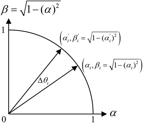respectively. The above formulation can be explained as follows. If the new $F$ is worse than $F^{\ast }$ and the bit state in $\mathit{b}$ is zero when the corresponding bit state in ${\mathit{b}}^{\mathbf{\ast }}$ is one, then a change in this bit from one to zero may worsen the fitness, and $\mathrm{\Delta }{\theta }_i$ is made negative to increase the corresponding ${\alpha }_i$ value (increasing the probability that the bit is in the “1” state, refer to Figure 1). In contrast, if the new $F$ is worse than $F^{\ast }$ and the bit state in $\mathit{b}$ is one while the corresponding bit state in ${\mathit{b}}^{\mathbf{\ast }}$ is zero, then $\mathrm{\Delta }{\theta }_i$ is positive, reducing the corresponding ${\alpha }_i$ value.

Figure 1. Plot of qubit update.

2.2. Quantum CNN

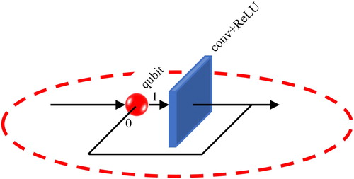
2.2.1. Quantum convolution unit

The quantum convolution unit (shown in Figure 2) is the new connection architecture proposed in this paper. It combines a qubit and a convolutional layer (which can contain other components, such as ReLU and batchNormalization), and the qubit determines whether the convolutional layer exists. When the qubit generates a binary bit “1”, this means that the convolution layer exists; otherwise, it means that the convolution layer does not exist.

Figure 2. Quantum convolution unit.

2.2.2. Quantum CNN architecture

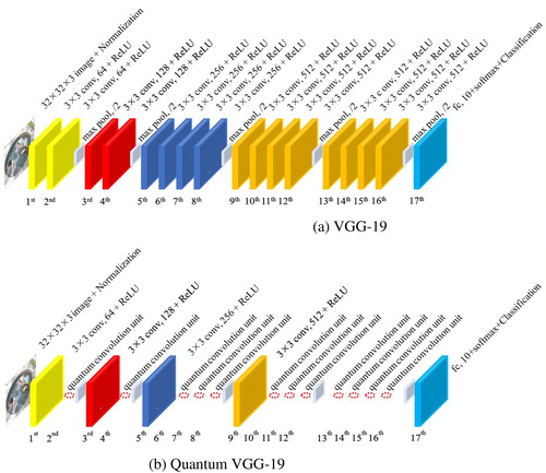
In CNN, the number of filters (kernels) in the convolutional layer determines the number of output feature maps, and also affects the depth of filters in the next layer of the convolutional layer. In other words, there is a problem of parameter dimension matching between convolutional layers, and not every convolutional layer can be arbitrarily removed during the optimisation process. When the number of filters in the convolutional layer is the same as that in the previous layer, the filter depth of the next layer remains the same. At this time, removing this convolutional layer does not cause the problem of parameter dimension mismatch. On the contrary, when the number of filters in the convolutional layer is different from the number of filters in the previous layer, the filter depth of the next layer is changed accordingly, and this convolutional layer cannot be removed. We call the immovable convolutional layers “immovable layers”. In addition, the remaining layers are replaced by the quantum convolution units, and qubits are used to determine whether the convolutional layers exists. Therefore, any CNN can be expressed as a quantum CNN architecture with the immovable layers and the quantum convolution units, and use this architecture to optimise the convolutional layers. Taking VGG-19 (Deng et al., 2016) in Figure 3(a) as an example, the number of convolutional layer filters of the first to second, third to fourth, fifth to eighth, and ninth to sixteenth layers are 64, 128, 256, and 512, respectively. So, the first, third, fifth, and ninth are immovable layers, the remaining layers are replaced by quantum convolution units, as shown in Figure 3(b).

Figure 3. VGG-19 and quantum VGG-19 (“N×N conv, n + ReLU” represents a convolutional layer containing n N×N filters and a rectified linear unit, “max pool, /2” represents a max pooling with a stride of 2, and “fc, 10+softmax + Classification” represents a fully connected layers with a 10-class softmax output).

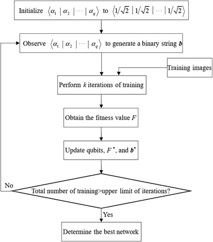
2.2.3. Quantum CNN optimisation process

This section explains how to use the quantum CNN architecture to optimise the convolutional layers. The training process is shown in Figure 4. Details of the initialisation, observation, and update are described below. If there are $q$ quantum convolution units in a quantum CNN, it means that there are $q$ convolution layers to be optimised. At this time, we can use a qubit individual with $q$ qubits $〈\begin{array}{ccccccc}{\alpha }_1& & {\alpha }_2& & \cdots & & {\alpha }_q\end{array}〉$ to represent this quantum CNN. In the initialisation stage, $〈\begin{array}{ccccccc}{\alpha }_1& & {\alpha }_2& & \cdots & & {\alpha }_q\end{array}〉$ is initialised to $〈\begin{array}{ccccccc}1/\sqrt{2}& & 1/\sqrt{2}& & \cdots & & 1/\sqrt{2}\end{array}〉$, which means that the probabilities of producing the binary “1” are all $1/2$. Next, the qubits are “observed” to generate a binary string $\mathit{b}$ and then obtain a candidate network architecture. To obtain the fitness value, we perform $k$ iterations of training on the candidate architecture, and let the training error be the fitness value $F$. In the update operation, the new training error (i.e. $F$) is compared with the stored best training error $F^{\ast }$. If $F<F^{\ast }$, $F^{\ast }$ and ${\mathit{b}}^{\mathbf{\ast }}$ are updated as $F$ and $\mathit{b}$, respectively. Otherwise, ${\alpha }_i$, i = 1, 2, … ., $q$, is updated using (3) and (4). Next, the qubits are observed again and generate a new candidate network until the total number of trainings reaches the upper limit of the specified number of iterations.

Figure 4. Quantum CNN training process.

3. Results and discussion

The method proposed in this paper is mainly aimed toward optimising feasible CNNs by which to make the network architecture simpler and improve its recognition accuracy, rather than pushing for state-of-the-art results. The simulation is mainly divided into two parts. First, we optimise the famous VGG-19 network, and the second part discusses the optimisation effect of the 20∼56 layer network. The experiments were performed on the CIFAR-10 dataset (Krizhevsky, 2009), which consists of 50k training images and 10k test images in 10 classes.

3.1. Quantum VGG-19

First, we optimise the VGG-19 (as shown in Figure 3(a)), for which its quantum architecture is shown in Figure 3(b). In the simulation, all training images are arbitrarily shifted up and down, left and right by 0–4 pixels, and are inverted with a 50% probability. We used stochastic gradient descent with a mini-batch size of 128. The learning rate starts from 0.01 and is divided by 10 every 23,400 iterations. The models are trained for up to 62,400 iterations, and the network structure is updated every 390 iterations (i.e. k = 390 in Figure 4). $\mathrm{\Delta }\theta$ in equation (4) affects the convergence speed of a quantum bit. Convergence may occur prematurely if this parameter is set too high (Moriyama et al., 2017, november). A value from $0.01\pi$ to $0.05\pi$ is recommended for the magnitude of $\mathrm{\Delta }\theta$ (Yang et al., 2004), although it depends on the problem. In the experiments, $\mathrm{\Delta }\theta$ was set to $0.05\pi$.

Table 2 shows the classification results of CIFAR-10 images obtained using the conventional VGG-19 and the quantum VGG-19 under the above training conditions. It can be seen from the table that the optimisation of the convolutional layer improves the test accuracy of VGG-19 by about 1.4%, and the average number of layers is also reduced by as much as 11 layers, which means that the number of VGG-19 weights can be reduced by nearly 60%.

Table 2. Comparison of original VGG-19 and quantum VGG-19 (average result of 5 runs).

	Number of layers	Test accuracy	Number of layers after training
VGG-19	19	90.5%	19
Quantum VGG-19		91.9%	7.2

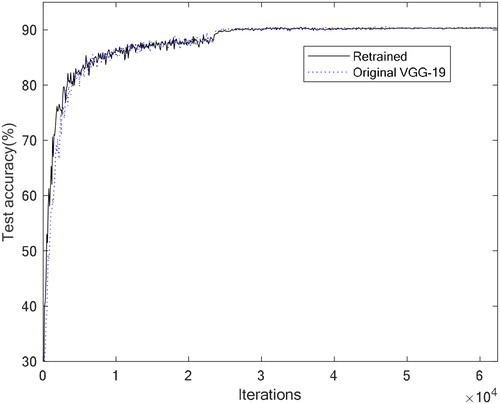
CNN uses the gradient descent method to update the weights. However, except for the initial weights (which are randomly generated at the beginning), the output of each subsequent step is predictable (it is also called the deterministic algorithm). In other words, the gradient descent method follows the same convergence trajectory, so it is not easy to escape from the local minimum (Juang & Hsu, 2009; Juang & Tsao, 2008; Srivastava & Biswas, 2020). This study uses qubits to change the network architecture during the weights convergence process, thereby changing the original convergence trajectory and finally leading to the opportunity to escape from the local minimum. Figure 5 shows the quantum VGG-19 optimisation result, for which test accuracy is approximately 91.9%. If we directly use the gradient descent method to retrain the weights of this architecture, its test accuracy becomes about 90.4%, which is no better than the original VGG-19 result, as shown in Figure 6 (since it has fewer layers, the initial convergence speed is faster than the original VGG-19). In other words, quantum CNN helps obtain better weight values.

Figure 5. Quantum VGG-19 optimisation result.

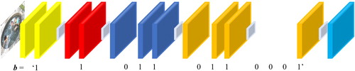
Figure 6. Retrain the weights under the architecture of Figure 5.

The main difference between QEAs and other optimisation algorithms is that QEAs can directly generate all possible solutions through “observation”, which is different from most population-based algorithms (such as genetic algorithms [Falahiazar & Shah-Hosseini, 2018; Oh et al., 2004], particle swarm optimizations [Kordestani et al., 2020; Nagra et al., 2020], etc.) that generate a new solution from individuals in the population. Take genetic algorithm as an example, to obtain the candidate network architecture of Figure 5, the population must have chromosomes containing some genes of “110110110001”, then be selected as the parents, and finally produce a child of “110110110001” through the crossover operations. However, if these genes are not included in the population, or the crossover point is not appropriate, it is impossible to obtain the desired result. However, using QEAs, the network architecture of Figure 5 can be obtained through observation at any time.

3.2. Other quantum CNNs

In order to further analyze the optimisation results of different layers of networks, we optimised the CNN networks of layers 20, 32, 44, and 56, respectively. The architecture is shown in Figure 7, where n = 6, 10, 14, and 18. According to the principle that the number of adjacent convolutional layer filters varies, the architecture of its quantum CNN can be designed as shown in Figure 8, in which the number of qubits is 16, 28, 40, and 52, respectively. Table 3 and Figure 9 show the average results of the original CNNs and the quantum CNN executed 5 times. As can be seen from the table, the average test accuracy of the original CNNs at 20 layers is about 89.8%, but as the number of network convolutional layers increases, the test accuracy gradually decreases. When the number of CNN layers reaches 56, the average test accuracy drops to about 83.4%, which means that too many convolutional layers not only require more computing resources, but also make the network’s prediction results worse. As for the quantum CNN, it not only has a better average test accuracy (about 91.5%) than CNNs at 20 layers, but when the number of layers gradually increases to 32, 44, and 56 layers, the average test accuracy can also be maintained at about 91%. This solves the problem of not knowing how many convolutional layers to choose when we first train the network. Since we define the training error of the network as the objective function, the architecture that produces the smallest training error is considered the best solution. Therefore, if the original network is large, the final optimised network may also be large. Even so, the original 56-layer network can reduce the number of layers to about 18 through QEA.

Figure 7. Multi-layer CNN architecture.

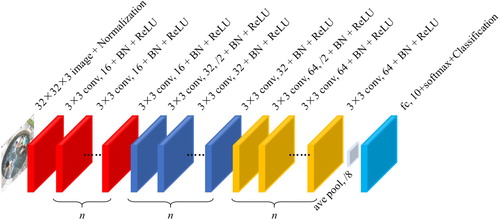
Figure 8. Quantum multilayer CNN architecture.

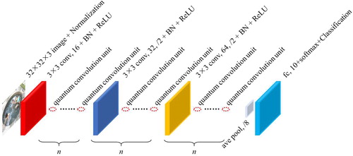
Figure 9. Comparison of test accuracy and number of layers.

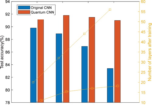
Table 3. Comparison of original CNN and quantum CNN (average result of 5 runs).

	Original layer	Test accuracy	Number of layers after training
CNN20	20	89.8%	20
Quantum CNN20		91.5%	11.0
CNN32	32	88.9%	32
Quantum CNN32		91.8%	15.4
CNN44	44	86.9%	44
Quantum CNN44		91.5%	17.0
CNN56	56	83.4%	56
Quantum CNN56		91.0%	18.2

4. Conclusions

This paper proposes a quantum CNN optimisation method that causes the network to try different network convolutional layer combination during the training process. This not only provides the opportunity to improve the problem of weights converging to a local minimum, but also improves the test accuracy of the network by eliminating the redundant convolutional layers. The simulations prove that regardless of VGG-19 or 20-layer, 32-layer, 44-layer, or even 56-layer CNN, the optimised network architecture through the QEA can be reduced by nearly half or more, and the test accuracy can be improved without being affected by the number of original network layers.

In this study, we consider the general CNN architecture, which has dozens of layers. In the future, a convolutional layer optimisation method for ResNet (over 100 layers) will be developed.

Disclosure statement

No potential conflict of interest was reported by the author(s).

References

- Bae, K. I., Park, J., Lee, J., Lee, Y., & Lim, C. (2020). Flower classification with modified multimodal convolutional neural networks. Expert Systems with Applications, 159, 1–11.
- Das, R., Piciucco, E., Maiorana, E., & Campisi, P. (2019). Convolutional neural network for finger-vein-based biometric identification. IEEE Transactions on Information Forensics and Security, 14(2), 360–373. https://doi.org/10.1109/TIFS.2018.2850320
- Deng, J., Dong, W., Socher, R., Li, L.-J., Li, K., & Fei-Fei, L. (2016, June). ImageNet: A large-scale hierarchical image database. In Proc. IEEE Int. Conf. Comput. Vis. Pattern Recognit. (CVPR) (pp. 248–255).
- Falahiazar, L., & Shah-Hosseini, H. (2018). Optimization of engineering system using a novel search algorithm: The spacing multi-objective genetic algorithm. Connection Science, 30(3), 326–342. https://doi.org/10.1080/09540091.2018.1443319
- Gao, Z., Wang, X., Yang, Y., Mu, C., Cai, Q., Dang, W., & Zuo, S. (2019). EEG-based spatio–temporal convolutional neural network for driver fatigue evaluation. IEEE Transactions on Neural Networks and Learning Systems, 30(9), 2755–2763. https://doi.org/10.1109/TNNLS.2018.2886414
- Garg, H. (2016). A hybrid PSO-GA algorithm for constrained optimization problems. Applied Mathematics and Computation, 274(11), 292–305.
- Han, K. H., & Kim, J. H. (2002). Quantum-inspired evolutionary algorithm for a class of combinatorial optimization. IEEE Transactions on Evolutionary Computation, 6(6), 580–593. https://doi.org/10.1109/TEVC.2002.804320
- Han, K. H., & Kim, J. H. (2006, July). On the analysis of the quantum-inspired evolutionary algorithm with a single individual. In Proc. of the 2006 Congr. on Evol. Comput. (pp. 2622–2629).
- He, K., & Sun, J. (2014, June). Convolutional neural networks at constrained time cost. In Proc. IEEE Conf. Comput. Vis. Pattern Recognit. (CVPR) (pp. 5353-5360).
- He, K., Zhang, X., Ren, S., & Sun, J. (2015, December). Delving deep into rectifiers: Surpassing human-level performance on imagenet classification. In Proc. IEEE Int. Conf. Comput. Vis. (pp. 1026–1034).
- He, K., Zhang, X., Ren, S., & Sun, J. (2016, June). Deep residual learning for image recognition. In Proc. IEEE Int. Conf. Comput. Vis. Pattern Recognit.(CVPR) (pp. 770–778).
- Ioffe, S., & Szegedy, C. (2015, July). Batch normalization: Accelerating deep network training by reducing internal covariate shift. In Proc. Int. Conf. Mach. Learn. (pp. 448–456).
- Juang, C. F., & Hsu, C. H. (2009). Reinforcement interval type-2 fuzzy controller design by online rule generation and q-value-aided ant colony optimization. IEEE Transactions on Systems, Man, and Cybernetics, Part B (Cybernetics), 39(6), 1528–1542. https://doi.org/10.1109/TSMCB.2009.2020569
- Juang, C. F., & Tsao, Y. W. (2008). A self-evolving interval type-2 fuzzy neural network with online structure and parameter learning. IEEE Transactions on Fuzzy Systems, 16(6), 1411–1424. https://doi.org/10.1109/TFUZZ.2008.925907
- Kim, M. G., Ko, H., & Pan, S. B. (2020). A study on user recognition using 2D ECG based on ensemble of deep convolutional neural networks. Journal of Ambient Intelligence and Humanized Computing, 11(5), 1859–1867. https://doi.org/10.1007/s12652-019-01195-4
- Kordestani, J. K., Meybodi, M. R., & Rahmani, A. M. (2020). A note on the exclusion operator in multi-swarm PSO algorithms for dynamic environments. Connection Science, 32(3), 239–263. https://doi.org/10.1080/09540091.2019.1700912
- Krasteva, V., Menetre, S., Didon, J. P., & Jekova, I. (2020). Fully convolutional deep neural networks with optimized hyperparameters for detection of shockable and non-shockable rhythms. Sensors, 20(10), 2875. https://doi.org/10.3390/s20102875
- Krizhevsky, A. (2009). Learning multiple layers of features from tiny images. Tech Report.
- Krizhevsky, A., Sutskever, I., & Hinton, G. E. (2012). ImageNet classification with deep convolutional neural networks. In Proc. Int. Conf. Neural Inf. Process. Syst. (vol. 60, pp. 1097–1105).
- Li, P., & Li, S. (2008). Learning algorithm and application of quantum BP neural networks based on universal quantum gates. Journal of Systems Engineering and Electronics, 19(1), 167–174. https://doi.org/10.1016/S1004-4132(08)60063-8
- Li, S., Ye, D., Jiang, S., Liu, C., Niu, X., & Luo, X. (2020). Anti-steganalysis for image on convolutional neural networks. Multimedia Tools and Applications, 79(7-8), 4315–4331. https://doi.org/10.1007/s11042-018-7046-6
- Liang, G., Hong, H., Xie, W., & Zheng, L. (2018). Combining convolutional neural network with recursive neural network for blood cell image classification. IEEE Access, 6, 36188–36197. https://doi.org/10.1109/ACCESS.2018.2846685
- Liao, G. P., Gao, W., Yang, G. J., & Guo, M. F. (2019). Hydroelectric generating unit fault diagnosis using 1-D convolutional neural network and gated recurrent unit in small hydro. IEEE Sensors Journal, 19(20), 9352–9363. https://doi.org/10.1109/JSEN.2019.2926095
- Liu, J., Chen, K., Xu, G., Sun, X., Yan, M., Diao, W., & Han, H. (2020). Convolutional neural network-based transfer learning for optical aerial images change detection. IEEE Geoscience and Remote Sensing Letters, 17(1), 127–131. https://doi.org/10.1109/LGRS.2019.2916601
- Lu, T. C., Yu, G. R., & Juang, J. C. (2013). Quantum-based algorithm for optimizing artificial neural networks. IEEE Transactions on Neural Networks and Learning Systems, 24(8), 1266–1278. https://doi.org/10.1109/TNNLS.2013.2249089
- Moriyama, Y., Iimura, I., & Nakayama, S. (2017, November). Investigation on introducing qubit convergence measure to QEA in maximum cup problem. In Proc. IEEE 10th Int. Workshop on Comput. Intelligence and Applications (pp. 73–78).
- Nagra, A. A., Han, F., Ling, Q. H., Abubaker, M., Ahmad, F., Mehta, S., & Apasiba, A. T. (2020). Hybrid self-inertia weight adaptive particle swarm optimization with local search using C4.5 decision tree classifier for feature selection problems. Connection Science, 32(1), 16–36. https://doi.org/10.1080/09540091.2019.1609419
- Nakazawa, T., & Kulkarni, D. V. (2018). Wafer map defect pattern classification and image retrieval using convolutional neural network. IEEE Transactions on Semiconductor Manufacturing, 31(2), 309–314. https://doi.org/10.1109/TSM.2018.2795466
- Oh, I. S., Lee, J. S., & Moon, B. R. (2004). Hybrid genetic algorithms for feature selection. IEEE Transactions on Pattern Analysis and Machine Intelligence, 28(11), 1424–1437.
- Rezaee, M., Mahdianpari, M., Zhang, Y., & Salehi, B. (2018). Deep convolutional neural network for complex wetland classification using optical remote sensing imagery. IEEE Journal of Selected Topics in Applied Earth Observations and Remote Sensing, 11(9), 3030–3039. https://doi.org/10.1109/JSTARS.2018.2846178
- Shao, G., Chen, Y., & Wei, Y. (2020). Convolutional neural network-based radar jamming signal classification with sufficient and limited samples. IEEE Access, 8, 80588–80598. https://doi.org/10.1109/ACCESS.2020.2990629
- Simonyan, K., & Zisserman, A. (2015, April). Very deep convolutional networks for large-scale image recognition. In Proc. Int. Conf. Learn. Represent. (ICLR) (pp. 1–14).
- Srivastava, V., & Biswas, B. (2020). CNN-based salient features in HSI image semantic target prediction. Connection Science, 32(2), 113–131. https://doi.org/10.1080/09540091.2019.1650330
- Sun, Y., Xin, Q., Huang, J., Huang, B., & Zhang, H. (2019). Characterizing tree species of a tropical wetland in southern China at the individual tree level based on convolutional neural network. IEEE Journal of Selected Topics in Applied Earth Observations and Remote Sensing, 12(11), 4415–4425. https://doi.org/10.1109/JSTARS.2019.2950721
- Szegedy, C., Liu, W., Jia, Y., Sermanet, P., Reed, S., Anguelov, D., Erhan, D., Vanhoucke, V., & Rabinovich, A. (2015, June). Going deeper with convolutions. In Proc. IEEE Int. Conf. Comput. Vis. Pattern Recognit. (CVPR) (pp. 1–9).
- Wang, X., Cheng, M., Wang, Y., Liu, S., Tian, Z., Jiang, F., & Zhang, H. (2020). Obstructive sleep apnea detection using ecg-sensor with convolutional neural networks. Multimedia Tools and Applications, 79(23-24), 15813–15827. https://doi.org/10.1007/s11042-018-6161-8
- Wang, M. M., Luo, J. J., & Walter, U. (2015). Trajectory planning of free-floating space robot using particle swarm optimization (PSO). Acta Astronautica, 112, 77–88. https://doi.org/10.1016/j.actaastro.2015.03.008
- Wu, H., Nie, C., Kuo, F. C., Leung, H., & Colbourn, C. J. (2015). A discrete particle swarm optimization for covering array generation. IEEE Transactions on Evolutionary Computation, 19(4), 575–591. https://doi.org/10.1109/TEVC.2014.2362532
- Yamashita, R., Nishio, M., Do, R. K. G., & Togashi, K. (2018). Convolutional neural networks: An overview and application in radiology. Insights into Imaging, 9(4), 611–629. https://doi.org/10.1007/s13244-018-0639-9
- Yang, H., Meng, C., & Wang, C. (2020). Data-driven feature extraction for analog circuit fault diagnosis using 1-D convolutional neural network. IEEE Access, 8, 18305–18315. https://doi.org/10.1109/ACCESS.2020.2968744
- Yang, S., Wang, M., & Jiao, L. (2004, June). A novel quantum evolutionary algorithm and its application. In Proc. Congr. Evol. Comput. (pp. 820–826).
- Yang, G., Zhou, F., Ma, Y., Yu, Z., Zhang, Y., & He, J. (2018). Identifying lightning channel-base current function parameters by Powell particle swarm optimization method. IEEE Transactions on Electromagnetic Compatibility, 60(1), 182–187. https://doi.org/10.1109/TEMC.2017.2705485
- Yu, X., Chen, W. N., Gu, T., Zhang, H., Yuan, H., Kwong, S., & Zhang, J. (2018). Set-based discrete particle swarm optimization based on decomposition for permutation-based multiobjective combinatorial optimization problems. IEEE Transactions on Cybernetics, 48(7), 2139–2153. https://doi.org/10.1109/TCYB.2017.2728120
- Zhang, F., Yang, F., Li, C., & Yuan, G. (2019). CMNet: A connect-and-merge convolutional neural network for fast vehicle detection in urban traffic surveillance. IEEE Access, 7, 72660–72671. https://doi.org/10.1109/ACCESS.2019.2919103
- Zhu, J., Chen, N., & Peng, W. (2019). Estimation of bearing remaining useful life based on multiscale convolutional neural network. IEEE Transactions on Industrial Electronics, 66(4), 3208–3216. https://doi.org/10.1109/TIE.2018.2844856
- Zhu, X., Zuo, J., & Ren, H. (2020). A modified deep neural network enables identification of foliage under complex background. Connection Science, 32(1), 1–15. https://doi.org/10.1080/09540091.2019.1609420