A dynamic network traffic classifier using supervised ML for a Docker-based SDN network

Abstract

With the rapid technological growth in the last decades, the number of devices and users has drastically increased. Software-defined networking (SDN) with machine learning (ML) has become an emerging solution for network scheduling, quality of service (QoS), resource allocations, and security. This paper focuses on the implementation of a network traffic classifier using a novel Docker-based SDN network. ML offers good performance to real-time traffic solutions without depending on well-known TCP or UDP port numbers, IP addresses, or encrypted payloads. In this paper, using three ML techniques, we first classify network flows with 3, 5, and 7 parameters giving up to 97.14% accuracy. Additionally, we present a new performance accelerator algorithm (PAA), which incorporates these three ML classifiers and accelerates the overall performance significantly. We then propose a dynamic network classifier (DNC) generated from PAA over a novel Docker-based SDN network. Finally, we propose a new controller algorithm for Ryu platforms, which integrates the DNC and classifies both TCP and UDP flows in real-time. Based on the evaluations, an improvement in latency performance has been demonstrated, where analysing a packet, controller processing time takes on an average of 10 µs. This study will certainly serve to further research on optimising SDN and QoS.

KEYWORDS:

• Quality of service
• software-defined network
• traffic classification
• machine learning

1. Introduction

In recent years, with the rapid growth of mobile communications, social networks, and new technologies, data traffic has exponentially increased (Cisco Visual Networking Index, 2018). New online games, video streaming, and other services have encouraged Internet service providers to optimise and adapt their network architectures to new technologies for offering better security, availability, quality of experience (QoE), and reliability to potential customers.

Software-defined network (SDN) is an emerging architecture that promises better performance and low latency. It is dynamically manageable, and ideal for high-bandwidth applications (David, 2020). SDN has attracted interest in networking by introducing the logical centralisation of control. It separates the control plane from the data plane, offering a global view of the network. Compared to traditional networks, SDN is easier to deploy, facilitates the implementation of network services, and offers scalable management within the networking infrastructure. To build SDN networks, researchers have focused their studies on existing SDN-supported NFV (Tseng et al., 2019) and emulators such as Mininet (n.d.), OFNet (n.d.), and Estinet (n.d.). Although Mininet emulator is widely used for working with OpenFlow (Open Virtual Switch, n.d.) virtual switches (OVS), it carries certain limitations in customising switches and adding applications to hosts. In this paper, we address this issue and propose a new Docker container-based virtual network.

Network administrators avoid investing in hardware resources, unless strictly necessary. They prefer maximising physical hardware by sharing computing power, storage, and memory capacity. Docker containers introduce a new way to deploy network applications into a portable image that runs anywhere and can be saved enhancing the user’s experience. Docker containers not only maximise the use of physical hardware, sharing of computing power, storage, and memory capacity but also facilitate communication and data sharing between cloud applications. They, as an open source platform, receive support from developers all around the world. By default, Docker containers can be interconnected in a linear-bus topology; complex topologies are not natively well supported and managed. In this paper, we have addressed the issue and proposed a way to support different complex topologies for Docker-based virtual network. However, SDN over the Docker platform implores attention for improvement and refinement.

To meet the steady demand of high transmission rates of internet, Network administrators need to design and configure a specific class of service (CoS) to offer better QoS. A well-designed network classifier (NC) is the key to implement effective management of network resources. It needs to be dynamic, scalable, and requires less human interaction. A network classifier identifies the type of application following some fields of header packets and patterns. With the increasing demand of network bandwidth, the rise of new dynamic applications and protocols network traffic classification is still a hot topic in network research.

There exist several works using port-based, payload-based, and machine learning-based techniques (Rezaei & Liu, 2020). Port-based works (Lopez et al., 2017) are no longer on hold since applications are using dynamic port number or ports from other applications. Payload-based works (Zhang et al., 2018), such as deep packet inspection (DPI), contain some limitations with pattern database updating, high time execution, and encryption techniques even though they possess high accuracy. Lastly, machine learning-based works are related to flow parameters obtained from header fields instead of ports or pay-load to predict the type of application.

Considering the limitations of traditional QoS, where the network administrators manually configure different access control lists (ACL) associated with IP addresses and port numbers, some works focused their studies on well-known ML techniques. However, with the increasing number of applications and classes of services, most of the previous work are no longer in hold. Moreover, there is a lack of implementation work in real environments or even in simulated platforms.

In this paper, we propose a new dynamic network traffic classifier (DNC) over a Docker-based SDN network, which presents a threshold analysis for mice and elephant traffic. Using our dataset, we analyse three ML techniques: Decision Tree (DT) (Burrows et al., 1995; Karatsiolis & Schizas, 2012; Quinlan, 1986), Random Forest (RF) (Breiman, 2001), and K-Nearest Neighbours (KNN) (Altman, 1992) for 3, 5, and 7 flow parameters. We present a new performance accelerator algorithm (PAA), which improves the accuracy as well as other performance metrics significantly. PAA integrates the pre-trained classifiers and creates the DNC that provides the best possible accuracy for each CoS. Finally, using 1, 3, 5, and 7 packets to the controller, we implement the DNC over Docker containers for TCP and UDP flows. We classify the flows into 1 of 10 CoSs and queued the traffic.

The main contributions are briefly summarised as follows:

1. We first extract 463,875 flows from 176 different applications to build a new dataset for training purposes. We then train three ML models to classify flows with 3, 5, and 7 parameters. Results indicate that proposed models perform effectively with seven parameters and can obtain up to 97.14% accuracy. In addition, we propose a new PAA algorithm, which combines the three ML classifiers and accelerates the overall accuracy up to 3.5%.

2. We reconfigure the existing Docker connection and build a new Docker-based virtual SDN network system for cloud applications that can follow any topology. Moreover, we propose a new controller algorithm for Ryu platforms. Evaluations with threshold (TH) of 1, 3, 5, and 7 packets demonstrate that both TCP and UDP flows can be classified in real time with a packet for mice and elephant traffic.

3. We conduct extensive tests in newly created Docker container-based virtual SDN networks to evaluate the performance of the proposed DNC. The simulation results indicate that controller processing time with the classifier has not been affected by consuming 10 µs on average.

The rest of the paper is organised as follows. Section 2 reviews related work and motivation. The new Docker-based network architecture, network classification process, and controller algorithm are described in Section 3. Section 4 presents the experiment setup for the simulation and prototype implementation. Section 5 discusses the evaluation results. Finally, Section 6 concludes this paper by summarising the findings and discussing the future works.

2. Related work

This section reviews some of the recent works related to our works. Section 2.1 mainly discuss about SDN networks and recent works with Docker containers. Section 2.2 summarises several machine learning techniques applied for classifying network traffic.

2.1. SDN network and Docker containers

SDN has emerged as a solution against the limitations of the traditional network, offering flow scheduling, better network monitoring, and centralised control while reducing maintenance and upgrade costs (Cui et al., 2016). SDN has been adopted in Google web search’s network using openflow from 2010 (David, 2020), and open-source routing protocols such as Border Gateway Protocol (BGP) and Intermediate System to Intermediate System (ISIS). Since 2012, Google has been working on a 100% openflow network because of flexibility and low latency. To increase link efficiency between data centres, B4 has been implemented in Google’s backbone, which reduces WAN link utilisation by 30% (Alsaeedi et al., 2019) Although SDN has a promising future, it is quite expensive and difficult to configure and test an SDN environment composed of real devices (Abar et al., 2020). Hence, Docker container-based virtual network can be a good alternative for testing SDN architectures.

Docker containers have become a popular method for deploying cloud applications (Merkel, 2014), and recently, have been widely used in fog computing platforms (Ahmed & Pierre, 2020). Researchers have shown strong interests in Docker virtualisation (Bachiega, 2020), however, Docker containers are not commonly used in SDN, nor is there any active research on them as a virtual network. In this paper, we concentrate on the implementation of Docker network virtualisation to bridge the gap.

2.2. Traffic classifier using machine learning

Recently, several works have focused their studies on different ML techniques to classify the network traffic (Chokkanathan & Koteeswaran, 2018; Oliveira et al., 2016; Zhang et al., 2012). Using the dataset of Cambridge University (Moore et al., 2013), authors in (Yuan & Wang, 2016) have obtained 60–90% accuracy for decision tree algorithm. Only 28 different applications are classified with an overall accuracy of 85.98% for the SVM based STICK mechanism in (Liu et al., 2018). For some particular applications, they even obtain 99% accuracy. Whereas, using MLP with only 3 hidden layers, authors obtain more than 96% accuracy for 10 CoS in (Zhou et al., 2011). They propose a DNN model, which classifies over 200 mobile application traffic and achieves 93.5% accuracy. They use five features such as packet size, destination address, protocol, port, and TTL with 8-layer DNN model. An adaptive learning technique has been proposed in (Liu et al., 2019) for mobile network traffic where their main concentration is to obtain a lower classification error rate with less time consumption. All these previous works mainly concentrate on improving the accuracy of the classifiers. Moreover, only a few applications or classes of these models achieve more than 90% accuracy and none of these works considered integrating their models in SDN and focus on system implementation.

Feature sets play an important role in network traffic classification. Using five feature sets, authors in (Lopez et al., 2017) show that their model tends to provide low performance when the feature set contains (Abar et al., 2020) less parameters. An enhanced random forest algorithm is proposed in (Wang et al., 2015), where using 29 selected features and 12 classes of services, they obtain an F1-score of 0.3–0.95, although only three classes have values higher than 0.96. These works show that achieving high accuracy with less features and more applications is a challenging task. Hence, one of the main goals is to achieve high accuracy with less number of feature sets.

A well-developed mathematical analysis for semi-supervised ML has been proposed for SDNs to classify and re-route elephant flows in (Wang et al., 2016). However, their work lacks mice traffic analysis and system implementation. In (Amaral et al., 2016) several traditional ML algorithms have been used and their traffic classification architecture is adaptable for SDN-based networks. They have categorised 12 different application groups and the overall accuracy of those categories is 71.4–95.9%. Nevertheless, the accuracy of some of those categories failed to achieve satisfactory results additionally their work lacks implementation of the classifiers in a real network.

The above-mentioned works mostly focus on the accuracy improvement of network classification and lack of detailed analysis and implementation. A recent work shows the implementation of DNN based NC in Mininet (Xu et al., 2018). However, their proposed system needs to capture packets for 15 s to perform classification tasks, which is not feasible for real-time traffic such as VoIP.

This paper aims to address all the issues mentioned above and proposes DNC that outperforms previous works. Moreover, it is undoubtedly a hard task to implement the network traffic classifier in an SDN network. The proposed controller algorithm incorporates DNC in a new Docker container-based SDN system which shows significant improvement in latency.

3. Proposed system model and methods

To conduct the experiments we build a new Docker container-based SDN network. Section 3.1 briefly describes the architecture of the network. In Section 3.2, we discuss the dataset for network traffic classification. Section 3.3 talks about the training process of machine learning models whereas in 3.4 we explain the proposed method for improving the overall performance of the ml models. Finally, in Section 3.4 we propose the controller algorithm.

3.1. Network architecture

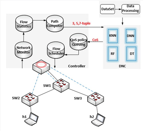
SDN is a dynamic and cost-efficient architecture, which decouples data and control planes (Latah & Toker, 2018). Its components are not required physically located in the same device or place. An SDN system mainly consists of three layers: infrastructure, control, and application. As shown in Figure 1, the infrastructure layer, or known as data plane, is responsible for data processing and forwarding using OpenFlow protocol.

Figure 1. SDN system architecture (API modules).

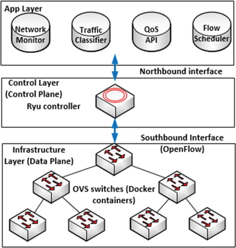
Control layer has an abstract network view. It receives requirements from applications and redirects them to the infrastructure layer, and vice versa. Finally, the application layer, via application programming interfaces (APIs), collects network information for making decisions. In this paper, we work with OpenFlow virtual switches, which are implemented over Docker containers. In this work, we use a Ryu controller (Ryu, n.d.) since it has all the latest features and supports rest API, python, and latest OpenFlow Switches. We integrate the proposed DNC in the Ryu controller as a QoS API in the application layer.

By default, in the general Docker network, the containers are interconnected via the Docker bridge, therefore, simple linear-bus topologies are well supported. However, other complicated topologies such as: binary tree, ring, mesh etc. are not well supported. To solve this problem, we first create a virtual Ethernet (veth) connection between two Docker containers and replace the user-defined Docker bridge (br0) with the newly created veth connection. We only keep one br0 that connects the Docker network to the external internet.

In Figure 2, we describe the Docker-based physical topology, which can be generated dynamically. Following a binary tree topology, we connect the Docker containers to a unique network using a user-defined Docker bridge (Br0). In the virtualised network system, the Docker containers are used as a virtual switches, controller and host application which is built on top of Ubuntu images. In order to make these containers act as switches, the Docker images need to have some unique features. Therefore, we modify the base Ubuntu images and create three types of Docker images:

1. For switch: Basic Ubuntu/CentOS with “supervisord” Docker and OVS,

2. For controller: Basic Ubuntu/CentOS with “supervisord” and Ryu controller,

3. For user applications: any Linux or Windows Distribution.

Figure 2. Physical topology of Docker-based SDN network.

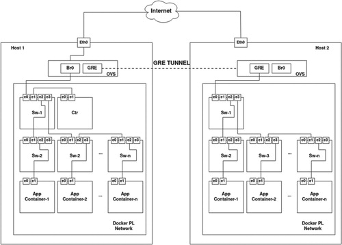
As shown in Figure 2, the first Docker container (sw-1), also known as the core switch of the network, has a link to the controllers as well as to the Docker bridge of the host. Multiple aggregation switches are attached to the core and the access layer (sw-2, sw-3, etc.). Finally, access switches are connected to application hosts. The controller (ctr) is physically connected to the core switch and has logical connection to all OVS switches in the cloud network. App containers (app-1, app-2, etc.) represent user devices, where host applications run. Using GRE tunnel, we connect multiple hosts containing Docker networks, which can be managed via a single controller as shown in Figure 2. For the experiments in this paper, we only work with a single Docker network in the same host.

Docker containers are lightweight and unlike virtual machines, they only use the user space of the operating system which saves a lot of hardware space. On the other hand, there are some simulators in market that can also virtualise network component. However, their simulation results are often inaccurate and they have other limitations. Hence, proposed container-based virtual Docker network can be a good alternative. Although, due to the hardware limitations our novel network still unable to support an extremely large network and we consider this issue as a future study.

3.2. Data set

One of the main contributions of this paper is the dataset. The vast majority of the previous datasets are now outdated because of the rise of new applications and mechanisms. For the pre-training stage of the classifiers, we require an unlabelled dataset from a laboratory-like network. We generate and capture real-time data traffic from our research laboratory, which is the backbone network for over 60 researchers with a small datacentre for testing applications.

Using a mirror port in the core switch of our laboratory network, we extract a 68.2 GB data file with unbalanced frequency distribution. Since this network traffic is unlabelled, we use nDPI, the Open Source DPI Library from ntop (Deri et al., 2014), to analyse the header and payload of the packets and generate labelled data. nDPI supports session certificates, allowing it to inspect many encrypted protocols (Bujlow et al., 2015). Although it has its own limitations, nDPI is a good approximation for traffic classification.

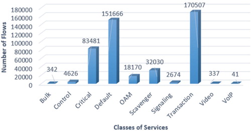
Each packet in the network belongs to a traffic flow, which has common parameters such as source address, and unicast, anycast or multicast destination address, source and destination port numbers, transport protocol, and others (Rezaei & Liu, 2020). This unique combination of parameters defines the connection and behaviour in the network. We extract 463,874 flows from 176 different applications. The obtained number of flows per CoS has been presented in Figure 3. Transactional, default, and critical data are the CoSs with more quantity of flows in the dataset. Since the data set is imbalanced, we used SMOTE (Chawla, 2002) technique to solve the problem. We only used SMOTE technique during the training phase, for testing and validation we used the actual data.

Figure 3. Number of flows in dataset for each CoS.

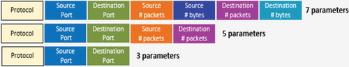
We decrypted the flows using nDPI and each flow contained more than 30 parameters. Most of these feature parameters are irrelevant to our classification task. Using “selectkbest” and “chi2” (Liu, 1995) algorithms, we, therefore, carry out feature selection task and select the seven most important features. Eventually, we build the dataset containing: source port, destination port, number of source-destination packets, source-destination bytes, number of destination-source packets, and destination-source bytes parameters as described in Figure 4. Moreover, we have repeated the same analysis for 3 and 5 parameters. We have excluded source and destination IP addresses since they hardly add any extra value to the classification.

Figure 4. Features of a network flow.

Finally, we include a description field about the related CoS associated with the applications. The flows are categorised into 10 different CoS (Aguirre et al., 2013), where network protocols and real-time traffic are our priority versus critical and bulk data. The unknown flows that nDPI fail to label are considered as default class traffic. The different CoS and applications are summarised in Table 1.

Table 1. Class of services and applications.

Class of services	Applications
Network control	ICMP, NTP, ICMPv6, IGMP,RTP
VoIP	SkypeCall, WhatsAppVoice
Multimedia streaming (video)	Youtube, AmazonVideo
Mission critical data	DNS, LLMNR, DHCP, DHCPV6, NetBIOS
Signaling	TLS, QUIC, H323, STUN.SkypeCall, STUN.Signal
Operations, administration and management (OAM)	SSH, TELNET, SNMP, UPnP, SSDP, BJNP
Transactional data	HTTP, HTTPS, RDP, TeamViewer
Bulk data	FTP, Backups, Email, Social Media, Instant messaging
Scavenger	BitTorrent, Gaming, Torrent, ApplePush
Best effort	Unclassified traffic, SSDP, UPnP, Broadcast, Mining

3.3. Training process

In this section, we discuss the training process and setup work with different machine learning techniques including DT, RF, and KNN. We also propose a new performance accelerator algorithm in Section 3.4, which significantly improves the overall performance of our models. While training the models we use 67% of the total data for training and 33% of total data for testing.

DT is a popular supervised machine learning technique. It follows a tree structure where the leaf nodes are the class label and the other unlabelled nodes are the features. DT is widely used because of its simplicity and high performance accuracy. CART (Burrows et al., 1995), ID3 (Quinlan, 1986), and C4.5 (Karatsiolis & Schizas, 2012) are the most commonly used DT algorithms. C4.5 algorithm performs well with the statistical data. Therefore, we choose this DT algorithm with 10 random states as our model.

DT already outperforms the accuracy of previous work. It has a tendency to over-fit some of the classes. Moreover, f1-score of some of the classes are not satisfactory. We, therefore, use RF, which is made up of many DTs. When building the trees, RF algorithm takes random samples of training data points. In order to split the nodes, they construct random subsets of features. For the purpose of training the model, we fix the max depth and random state of the RF to 10 and 15 to reduce the over-fitting. Tables 4 and 5 show overall accuracy and other performance scores, respectively.

In general, RF performs better than DT, however, RF’s f1-score for VoIP, signalling and bulk data is comparatively lower than the other classes. Hence, we adopt KNN algorithm in this work.

KNN algorithm is well-known for classifying the sample data based on the nearest neighbour of unclassified data. We have tried various k-values, concluding that k = 3 is the best outcome. Table 4 demonstrates that KNN gives better overall accuracy in comparison to RF. KNN gives the best accuracy and considerably good f1-score for most of the classes.

While training these models, we noticed that no single model can outperform others. DT and RF’s overall accuracy is less than KNN but for some particular classes, the accuracy and f1-score are slightly better. Since there is no particular model that can outperform others, we propose the PAA algorithm that significantly improves the overall accuracy and f1-score for each class.

3.4. Performance accelerator algorithm (PAA)

From the confusion matrix of Figure 8, we can notice there is no universal ML algorithm that outperforms results for all classes. RF can classify OAM, and transaction classes better than DT, and KNN. Similarly, for video, VoIP, bulk, and signalling data, KNN offers good performance. DT performs best for control and critical data. Therefore, we propose the following algorithm for pre-trained models, which finds the best performance for each class and predicts classes accordingly.

Let, m be the number of pre-trained classifiers. Then, $X^m$ is the set of base level pre-trained machine learning classifiers, $X^m=\{X^1,X^2,\dots ,X^m\}$ for our experiment m = 3. Let, $f(X^m)=Y^m$ then, $Y^m$ is the set of output data for each pre-trained classifier. Using the original dataset D, we construct a new dataset D_N. Let’s assume we have n data points in the original dataset then, D_{N = 1, 2, 3  …  ., n}. Then, a new data point, $D_{N=1}=\{Y_1^1,Y_1^2,\dots ,Y_1^m,Y_1\}$ where Y₁ denotes the actual output for N = 1.

Using the new dataset D_N, we train a DNN model as the meta classifier with an input, an output and four hidden layers. Each hidden layer has Rectified Linear Units (ReLU) and the output layer has Softmax as activation functions. For avoiding overfitting, we add L2 regularisation in the third hidden layer. We use Adam optimiser with a learning rate of 0.001. Since this is a multi-class classification problem, we choose Sparse Categorical Cross Entropy as the loss function of the model. If we consider $y_i$ as our actual output and $\widehat{y_i}$ as our predicted output, then the goal is to minimise the loss function (1). We train the model between 10 and 30 epochs with a batch size of 200. (1) $J(w)=-\frac{1}{N}\sum _{i=1}^N[y_i\log (\widehat{y_i})+(1-y_i)\log (1-\widehat{y_i})]$(1)

The proposed algorithm (Algorithm 1) follows three main steps which can be described as follows:

1. First we take the original training data as input. Next, we train some base-level classifiers with the data and make a set of them.

2. We then construct a new dataset based on the base level classifiers’ prediction. The output of the base level classifiers will be input for the meta classifier.

3. Finally, we train a DNN model as a meta classifier using the data in (2).

Proposed PAA, combines the pre-trained models and finds the best accuracy, precision, recall, and f1-score for each class. Finally, using the pre-trained classifiers and PAA algorithm, we create the DNC (Dynamic Network Classifier) and use as QoS API for the controller.

Table

Algorithm 1: Performance Accelerator Algorithm

1. D←Input: Training Data

2. H←Output: Trained Classifier

Step 1: learn base level classifiers

3. for t in T do [T is the set of given classifiers]

4. train ht based on D

5. end for

Step 2: construct new dataset based on base level classifiers’ prediction

6. for i to m do

7. ${\text{D}}_{\text{n}}=\{{\text{x}}_{\text{i}}^{\text{T}},{\text{y}}_{\text{i}}\};$ where ${\text{x}}_{\text{i}}^{\text{T}}$ is the output of base level classifiers, yi is the actual output

8. end for

Step 3: learn meta classifier

9. learn H based on Dn

10. return H

3.5. Controller algorithm

The QoS policy queuing API is responsible for classifying and routing the data traffic. Using DNC-based QoS API, packets are classified into 1 of the 10 CoS from Table 1. Once flow features are identified, we add the new flow entry in the flow table of the OVS switches and associate the special QoS treatment with the queueID.

As shown in Figure 5, the application layer mainly consists of 6 modules (Zhang et al., 2018). Network monitoring module analyses the network information such as protocol, and source and destination ports. Flow statistics is a module to collect flow information and statistics (e.g. number of packets of the flow and duration time). Whereas, the path computer is responsible for calculating the shortest path to the destination. During training, a data processing module collects flow information and builds the training set. DNC receives 3, 5, or 7 parameters as input and responses with predicted CoS. QoS policy queuing module will associate the CoS with the queue and specify the treatment with which flow will be linked. Finally, the flow scheduler module is responsible for building flows and adding them in the flow table of every OVS switch of the network.

Figure 5. API modules of the designed system.

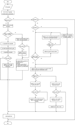
The algorithm of how the controller and network traffic classifier work is described as follows.

When a new packet arrives, the first OVS switch checks if there is a matched flow entry. If there is, the packet is sent out to its destination, otherwise, it is sent out to the controller.

Controller receives the packet and calculates the shortest path to the destination. If source and destination hosts are connected to the same OVS switch, we obtain a path equal to 1. Otherwise, more switches are involved. If path length is bigger than 2, controller will configure the flows following the next fixed order to guarantee that flow path is fully configured when source flow is added. First, in the intermediate switches, then the destination switch, and lastly the source switch. If path is equal to 2, only two OVS switches are involved. Configurations are made first in the destination and then in the source switch.

Network classifier receives 3, 5, or 7 parameters in every test, respectively, to predict the CoS, and returns a queue ID. Packets which are unable to be classified are considered in the default queue with less priority (queue ID 9).

Controller associates the queue ID with the output port as actions in the flow entry. Moreover, it checks if the threshold condition (1, 3, 5, or 7 packets) has been fulfilled before inserting the flow in the source switch. If there are less packets than the threshold requires, the flow is not added in the OVS switch table. However, the packet is successfully sent out to the destination with best effort treatment. With this condition, we guarantee that not only mice traffic arrives at the destination anytime but also a better prediction for elephant traffic.

Finally, flow is added to the flow table of every OVS switch for that specific data path. New packets of the same flow can be received by the switches and routed to the destination with the specific treatment.

More details are described in Algorithm 2 and Figure 6.

Figure 6. Flowchart of controller scheduling and CoS allocation algorithm.

Table

Algorithm 2: Controller scheduling and CoS allocation

1. Input: ipv4 packets

2. Output: send packets to destination

3. threshold TH = 1, 3, 5 or 7 packets

4. calculate the shortest path to destination

5. if (path includes a switch)

6. obtain in/out ports from the same switch

7. if (packet is UDP or TCP)

8.  Obtain queue ID from classifier output

9.  insert flow with in_port in the flow table

10.  if (reaches the TH)

11.   repeat 8-9 with out_port, priority 1

12.  end if

13. end if

14. else

15.  for other traffic, repeat 8-9 with in_port, priority 1

16.  if (reaches the threshold TH)

17.   repeat 8-9 with out_port, priority 1

18.  end if

19.  send traffic to controller

20.  repeat 9, with priority 2

21. end else

22. end if

23. else if (path $\ge$2 switches)

24. if (path>2 switches)

25. for (each middle switch in the path, insert the flows)

26.  obtain out_port from every switch

27.  if (packet is UDP or TCP)

28.   repeat 8-9 with out_port, priority 3

29.  end if

30. end for

31. end if

32. else

33.  repeat 8-9 with out_port, priority 1

34. end else

35. Obtain in/out ports from the source switch

36. Obtain in_port from the destination switch

37. if (packet is UDP or TCP)

38.  repeat 8-9 with in_port_dst, priority 3

39.  if (reaches the threshold TH)

40.   Insert the flow in the source switch at the end, repeat 8-9 with out_port_src, priority 3

41.  end if

42. end if

43. else

44.  repeat 8-9 with in_port_dst, priority 1

45.  if (reaches the threshold TH)

46.   repeat 8-9 with out_port_src, priority 1

47.  end if

48.  send traffic to controller

59.  repeat 9 with priority 2

50. end else

51. end else if

52. send packet to destination

4. Experiment setup

For data processing, we use python Numpy and Pandas libraries. For training DT, RF and KNN models, we work with scikit-learn (Pedregosa et al., 2011) library. For the DNN model, we use Keras library provided by Tensorflow python package. We train the models in a 64-bit Windows 10 OS based personal PC with Intel(R) Core(TM) i5-7500, CPU3.40 GHz, RAM 16 GB.

The prototype of the network has been implemented in a server (dual-core, Intel(R) Xeon(R)CPU E5-2630 [email protected] GHz, 264 GB RAM) running 6 Docker containers over Ubuntu OS (version16.04.1): 1 Ryu controller, 3 OVS switches, and 2 host applications, as shown in Figure 5.

In Table 2, we describe the corresponding per-hop behaviour (PHB) and differentiated services code point (DSCP). Although, we only use the queue ID when we configure a flow. Each queue has a maximum bandwidth, which has been configured in 40-Mbps output interfaces.

Table 2. Class of service and QoS parameters.

Class of services	PHB	DSCP	Queue	BW(Kbps)
Network control	CS6	48	0	1000
VoIP	EF	46	1	1000
Multimedia streaming	AF41	34	2	5000
Mission critical data	AF31	26	3	3000
Signaling	CS3	24	4	4000
OAM	CS2	16	5	3000
Transactional data	AF21	18	6	8000
Bulk data	AF11	10	7	6000
Scavenger	CS1	8	8	5000
Best effort	0	0	9	4000

In this work, we run OpenFlow 1.3 version in the three virtual switches. As shown in Figure 5, the core switch (sw-1) has an eth0 connection to the default gateway (main server), and the eth3 to the controller. Access layer switches (sw-2 and sw-3) have connections to sw-1 and host applications.

Table 3 shows CPU and memory statistics of each container in the Docker-based SDN network. A controller requires more hardware resources than the other Docker containers.

Table 3. Hardware statistics for Docker containers.

Name	CPU%	Mem usage/limit	CoS	PIDS
2S_ctr	2.48	228.3 MiB/251.7 GiB	Network control	ICMP, NTP, ICMPv6, IGMP,RTP
2S_sw-1	2.48	202.4 MiB/251.7 GiB	VoIP	SkypeCall, WhatsAppVoice
2S_sw-2	0.48	195.3 MiB/251.7 GiB	Multimedia streaming	Youtube, AmazonVideo
2S_sw-3	0.71	189.7 MiB/251.7 GiB	Mission critical Data	DNS, LLMNR, DHCP, DHCPV6, NetBIOS
2S_usr-1	0.00	125.1 MiB/251.7 GiB	Signaling	TLS,QUIC, H323, STUN.SkypeCall, STUN.Signal
2S_usr-2	0.00	76.62 MiB/251.7 GiB	OAM	SSH, TELNET, SNMP, UPnP, SSDP, BJNP

Moreover, we implement supervisord Dockers (Supervisord Docker, n.d.) to run multiple processes simultaneously for the database (ovsdb-server) and open vSwitch daemon (ovs-vsctl), although it increases memory usage in switches.

Finally, we deploy the system and classify the type of traffic with the mentioned parameters in Figure 4. In the prototype implementation, we associate the queue ID and outport in an action group to guarantee different treatment for every flow. For example, for ICMP traffic, which is control and high priority traffic (queue ID: 0), we obtain two unidirectional flows with actions: “group: 30” and “group: 20”. According to our standards, the first number represents the outport in the switch, and the second one, the queue ID (0). In this paper, we neither analyse any QoS scheduling nor congestion algorithms.

5. Evaluation

This section briefly reviews the experiment result of the proposed network traffic classifiers and the Docker-based virtual SDN network system. In Section 5.1 we summarise the performance of the classifiers. Section 5.2 shows the implementation results of the classifiers in the proposed Docker container-based virtual network system.

5.1. Network classifier simulation

In this section, we discuss the accuracy and performance of pertained classifiers and the DNC simulation. In order to measure the performance of the classifiers, we use the following performance metrics: accuracy, precision, recall, and f1-score.

Accuracy (2) is the ratio of total number of correctly classified components and the total number of sample components. (2) $Accuracy=\frac{(TP+TN)}{(TP+TN+FP+FN)}$(2)

Precision (3) is the ratio of the components that is correctly classified to a given component class. (3) $Precision=\frac{(TP)}{(TP+FP)}$(3)

Recall (4) is the ratio of the components belonging to a class that is correctly classified to that specific class. (4) $Recall=\frac{(TP)}{(TP+FN)}$(4)

F1-score (5) is the harmonic mean of precision and recall, defined as follows: (5) $F1\text{ - }score\text{ = }\frac{2\times (Precision\times Recall)}{(Precision+Recall)}$(5)

Table 4 depicts the average accuracy of DT, RF, and KNN algorithms for 3, 5, and 7 parameters. We can observe that KNN gives comparatively higher accuracy than DT and RF. It is also noticeable that the accuracy of the classifiers shows a correlation with the number of parameters. Therefore, we only use seven parameters for further evaluations.

Table 4. Accuracy of ML models for different number of parameters.

Parameters	DT (%)	RF (%)	KNN (%)
Protocol, src_port, des_port, src_packets, src_bytes, des_packets, des_bytes	95.80	96.69	97.14
Protocol, src_port, des_port, src_packets, des_packets	95.56	96.52	96.69
Protocol, src_port, des_port	87.64	89.90	94.82

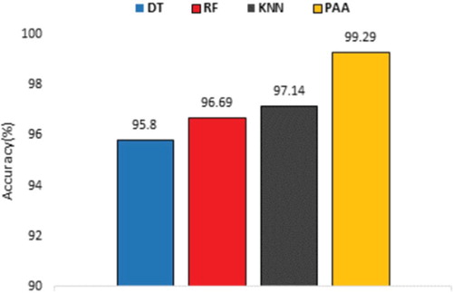
We can analyse that DT overall demonstrates 95.80% of accuracy, however, it has the tendency to over-fit. In such cases, RF imparts marginally better accuracy of 96.69%, which restrain the problem of overfitting. Although DT and RF have such higher overall accuracy, they fail to achieve satisfactory accuracy and f1-score. Therefore, we train a KNN model that detects VoIP and multimedia streaming data with better accuracy and an overall accuracy of 97.14%. Finally, Figure 7 demonstrates that proposed PAA achieves 99.29% accuracy, and as the epoch goes higher, the accuracy slowly increases in.

Figure 7. Accuracy versus epochs for PAA model.

From Table 5, we can calculate the macro average precision, recall and f1-score for 7 parameters of the classifiers. Among the three traditional classifiers, KNN demonstrates the best results: precision, recall and f1-score respectively 68%, 98%, and 77%. DT and RF show almost similar scores however, RF has a slightly higher recall of 98%, but the lower precision affects the overall f1-score. It is also observable that most classes have more than 90% f1-score for DT, RF, and KNN. However, there is no single model that outperforms others in each class. The CoSs such as multimedia streaming, bulk, and VoIP obtain significantly lower performance scores than other classes. Moreover, confusion matrices of DT (Figure 8(a)), RF (Figure 8(b)), and KNN (Figure 8(c)) indicate that VoIP traffic is mistakenly classified as transactional data, scavenger and default classes. Mainly, because these classes have similarities in their behaviours.

Figure 8. (a) Confusion matrix of DT for seven parameters. (b) Confusion matrices of RF for seven parameters. (c) Confusion matrices of KNN for seven parameters. (d) Confusion matrices of DNC for seven parameters.

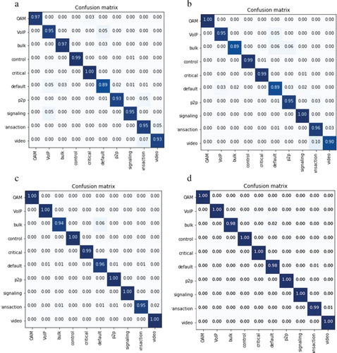
Table 5. Comparison of precision, recall, and F1-score for DT, RF, KNN, and PAA.

	DT			RF			KNN			PAA
Class of service	Precision	Recall	F1-score	Precision	Recall	F1-score	Precision	Recall	F1-score	Precision	Recall	F1-score
OAM	0.99	0.97	0.98	0.97	1.00	0.98	0.94	1.00	0.96	1.00	1.00	1.00
VoIP	0.05	0.95	0.09	0.08	0.95	0.15	0.19	1.00	0.32	0.50	0.91	0.65
Bulk data	0.15	0.97	0.26	0.15	0.89	0.26	0.18	0.97	0.30	0.60	0.92	0.73
Network control	1.00	0.99	0.99	1.00	0.99	0.99	0.89	0.99	0.94	0.99	1.00	1.00
Mission critical data	1.00	1.00	1.00	1.00	0.99	1.00	1.00	1.00	1.00	1.00	1.00	1.00
Best effort	0.99	0.89	0.94	0.99	0.89	0.94	0.99	0.96	0.97	0.99	0.98	0.99
Scavenger	0.78	0.93	0.85	0.68	0.95	0.80	0.85	0.99	0.91	0.93	1.00	0.96
Signaling	0.24	0.95	0.38	0.12	1.00	0.21	0.48	1.00	0.65	0.85	0.98	0.91
Transactional data	0.99	0.95	0.97	0.99	0.96	0.98	0.99	0.95	0.97	0.99	0.99	0.99
Multimedia streaming	0.22	0.93	0.35	0.34	0.90	0.49	0.47	0.99	0.64	0.79	0.92	0.85

These results prove that no individual model can offer the best performance for every class. Therefore, we propose PAA to improve the overall performance of the models. Comparing PAA with the individual model’s accuracy, the former shows an accuracy improvement of 2–3.5% as shown in Figure 9. Moreover, PAA also improves other performance metrics including f1-score. Table 5 shows us among the four models, PAA gives the best f1-score value for any of the 10 CoS. Finally, we conducted a simulation test that indicates DT, RF, and KNN consume only 3 ms on average to classify a flow. However, PAA takes 20 ms, which is slightly higher than others but offers significant improvements in overall performance.

Figure 9. Accuracy of PAA versus other ML models.

5.2. Network classifier implementation

In this section, we present and analyse the results obtained in the DNC implementation. In order to prove that DNC can classify traffic data without increasing the latency considerably, we run tests using ping, iperf, and SSH, and obtain the controller processing time of 10 µs on average per packet for each application as shown in Figure 10.

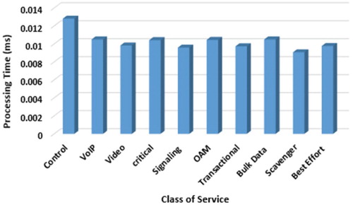
Figure 10. Average processing time per CoS.

We evaluate different parameters such as delay, packet loss, jitter, and bandwidth for TH values of 1, 3, 5, and 7 packets. To create a better comparison, we conduct the same tests without NC. We implement the prototype with seven parameters as shown in Figure 4 and execute the proposed PAA algorithm and create DNC. The evaluations are described as follows.

5.2.1. Control class: ICMP

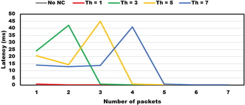
Using ICMP, we check connectivity between host 1 and host 2 for 100 packets. As shown in Figure 11, there is an initial time, which increases proportionally with the threshold. This variation is associated with the number of packets that DNC needs to process before a prediction.

Figure 11. Initial time for 1st–7th ICMP packets with no NC and 1, 3, 5, and 7 thresholds.

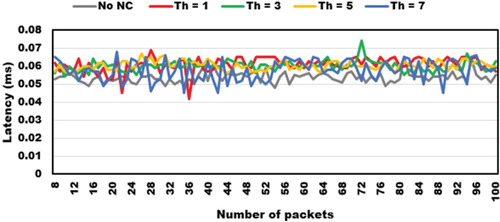
After the 7th and 8th packet, we can notice latency is similar for all tests because flow entries are already inserted in the flow tables (control class). On average, this value is 58.9 µs as shown in Figure 12.

Figure 12. Initial time for 8th–100th ICMP packets with no NC and 1, 3, 5, and 7 thresholds.

Finally, in Table 6, we summarise the results for packet loss, average initial time (1st–7th packets), average time (8th–100th packets), and total average time (1st–100th packets). We conclude that total average time is directly proportional to the number of thresholds. Controller requires more processing time when more packets need to be processed.

Table 6. Latency for control class packets.

Parameters	No NC	TH = 1	TH = 3	TH = 5	TH = 7
Packet loss (%)	0	0	0	0	0
Avg. initial time (ms)	0.1204	0.1321	9.5888	11.5830	11.7714
Avg. time (ms)	0.0538	0.0612	0.0602	0.0609	0.05795
Total Avg. time (ms)	0.0584	0.0660	0.2721	0.8670	0.8776

With these results, we assert that the proposed classifier with TH = 1 (66 µs) presents a similar latency to no NC (58.43 µs). On average, the increasing processing time difference is 7.6 µs.

5.2.2. Scavenger class: UDP/TCP Iperf

For this experiment, we use the Iperf command to send UDP and TCP traffic from host 1 to host 2 with 1 Mbps bandwidth.

We observe 0% packet loss and 1–2 ms jitter for UDP from Table 7. However, in Table 8 for TCP packets, we show bandwidth, transfer bytes and TCP windows size parameters. In conclusion, there are no notable differences with Iperf when threshold value changes.

Table 7. Network parameters for UDP scavenger class.

Parameters	No NC	TH = 1	TH = 3	TH = 5	TH = 7
Bandwidth (Mbps)	1.05	1.05	1.05	1.05	1.05
Transfer (Mbytes)	1.25	1.25	1.25	1.25	1.25
Jitter (ms)	0.002	0.001	0.001	0.001	0.002
Packet loss (%)	0	0	0	0	0
Diagrams	893	893	893	893	893

Table 8. Network parameters for TCP scavenger class.

Parameters	No NC	TH = 1	TH = 3	TH = 5	TH = 7
Bandwidth (Mbps)	1.1	1.12	1.15	1.14	1.14
Transfer (Mbytes)	1.38	1.38	1.38	1.38	1.38
Window size (KB)	85.3	85.3	85.3	85.3	85.3

We repeat this test more than 10 times for each threshold. We initially observed 1300 ms jitter and 50% packet loss. To mitigate these effects, we run a script to clean up flow and ARP tables in switches and hosts before each test.

5.2.3. OAM class: SSH

To generate OAM class traffic, we send an SSH request from host 1 to a server located outside of the Docker container network. From Figure 13(a), we can see that the processing time for OAM traffic without NC is on average 5.9 µs.

Figure 13. Controller processing time with no NC and 1, 3, 5, and 7 thresholds.

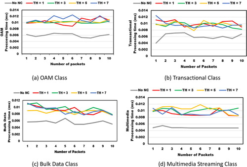
For TH = 1, 3, 5, and 7, we obtain averages of 10.3, 10.1, 10.2, and 10.1 µs respectively, after testing 10 packets. We can conclude that the average processing time of the controller using DNC is 10.4 µs, which is hardly perceptible for OAM traffic.

5.2.4. Transactional, bulk, and multimedia streaming classes: Firefox HTTP

We faced some hindrances in running this test since the server lacked graphics card. During this evaluation, we open Baidu search engine and obtain different packet flows. In Figure 13(b), we show the generated HTTP and HTTPS traffic classified as transactional data. We obtain 10, 9.4, 9.7, and 9.6 µs for TH equal to 1, 3, 5, and 7 respectively. We can conclude that 9.7 µs is the average processing time for OAM traffic. With no NC, we obtain 6 µs on average since it does not classify traffic.

In Figure 13(c), we identify a similar behaviour for bulk data class. We obtain 9.1, 9.5, 8.6, and 9 µs for a threshold of 1, 3, 5, and 7 respectively. The average processing time for bulk data is 9 µs while without NC is 5 µs. For multimedia streaming class, we test Amazon video packets and obtain 9.2, 10.1, 10.4, and 9.4 µs for 1, 3, 5, and 7 packet threshold as shown in Figure 13(d). The average processing time is 9.8 µs while without NC is 4.9 µs. Similar results have been observed while testing the other classes.

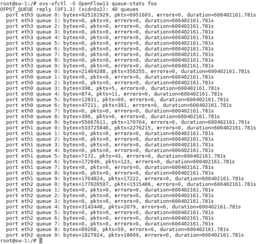
Figure 14 shows the queue statistics in the core switch (sw-1) of the network. For each Ethernet port, we have 10 queues which represent 10 CoS. In the figure, we can notice how our proposed system classifies the network traffic and put it in the queues. Based on the priority of the queue the network traffic will get proper treatment. Finally, with the experimental results of the prototype we conclude that the processing time of the controller is relatively similar to that of not using a classifier. Since the processing time of the controller hardly affects the system, we, therefore, strongly consider working with a packet and seven parameters as the accuracy for the proposed DNC is reaches up to 99.29%.

Figure 14. Queue statistics of network traffic in core switch (sw-1).

6. Conclusion

In this paper, we have introduced the design and evaluation of DNC for a SDN-based network. Using three ML techniques, we classify TCP and UDP flows with 3, 5, and 7 parameters giving up to 97.14% accuracy. We then present a new PAA, which is capable of combining different ML models and accelerating the accuracy up to 3.5%. Additionally, using PAA we get DNC that shows significant improvements in overall performance. In order to evaluate the performance, we introduce a new Docker-based SDN network system and implement the proposed DNC in a Ryu controller removing the burden of matching the incoming traffic manually and ensuring better QoS. Experiment results demonstrate significant improvement in latency performance in which analysing a packet takes a controller processing average time of 10 µs. Moreover, we plan to introduce a multi-cluster controller, scheduling, and congestion algorithms in our system as future work.

Disclosure statement

No potential conflict of interest was reported by the author(s).

Additional information

Funding

This work was partially supported by the Research and Development Projects of Applied Technology of Inner Mongolia Autonomous Region, China under grant number 201802005, the Key Program of the National Natural Science Foundation of China under grant number 61932014, and Pudong New Area Science & Technology Development Fund under Grant No. PKX2019-R02.

References

- Abar, T., Letaifa, A. B., & Asmi, S. E. (2020). Quality of experience prediction model for video streaming in SDN networks. International Journal of Wireless and Mobile Computing, 18(1), 59–70. https://doi.org/10.1504/IJWMC.2020.104769
- Aguirre, L. P., González, F., & Mejía, D. (2013). Aplicaciones de MPLS, transición de IPv4 a IPv6 y mejores prácticas de seguridad para el ISP Telconet. Revista Politécnica, 32, 43–51. https://revistapolitecnica.epn.edu.ec/ojs2/index.php/revista_politecnica2/article/view/40
- Ahmed, A., & Pierre, G. (2020). Docker-pi: Docker container deployment in fog computing infrastructures. International Journal of Cloud Computing (IJCC), 9(1), 6–27. https://doi.org/10.1504/IJCC.2020.105885
- Alsaeedi, M., Mohamad, M., & Al-Roubaiey, A.-R. (2019). Toward adaptive and scalable OpenFlow-SDN flow control: A survey. IEEE Access, 7, 107346–107379. https://doi.org/10.1109/ACCESS.2019.2932422
- Altman, N. S. (1992). An introduction to kernel and nearest-neighbor nonparametric regression. The American Statistician, 46(3), 175–185. https://www.tandfonline.com/doi/abs/10.1080/00031305.1992.10475879
- Amaral, P., Dinis, J., Pinto, P., Bernardo, L., Tavares, J., & IEEE. (2016). Machine learning in software defined networks: Data collection and traffic classification. In 2016 IEEE 24th International Conference on Network Protocols (ICNP) (pp. 1–5). Singapore, Singapore.
- Bachiega, N. G. (2020). Performance evaluation of container’s shared volumes. In 2020 IEEE International Conference on Software Testing, Verification and Validation Workshops (ICSTW). Porto, Portugal.
- Breiman, L. (2001). Random forests. Machine Learning, 45(1), 5–32. https://doi.org/10.1023/A:1010933404324
- Bujlow, T., Carela-Español, V., & Barlet-Ros, P. (2015). Independent comparison of popular DPI tools for traffic classification. Computer Networks, 76, 75–89. https://doi.org/10.1016/j.comnet.2014.11.001
- Burrows, W. R., Benjamin, M., Beauchamp, S., Lord, E. R., McCollor, D., & Thomson, B. (1995). CART decision-tree statistical analysis and prediction of summer season maximum surface ozone for the Vancouver, Montreal, and Atlantic. Journal of Applied Meteorology, 34(8), 1848–1862. https://doi.org/10.1175/1520-0450(1995)034<1848:CDTSAA>2.0.CO;2
- Chawla, N. V. (2002). SMOTE: Synthetic minority over-sampling technique. Journal of Artificial Intelligence Research, 16, 321–357. https://doi.org/10.1613/jair.953
- Chokkanathan, K., & Koteeswaran, S. (2018). A study on flow based classification models using machine learning techniques. International Journal of Intelligent Systems Technologies and Applications, 17(4), 467–482. https://doi.org/10.1504/IJISTA.2018.095114
- Cisco Visual Networking Index. (2018). Cisco visual networking index: Forecast and trends, 2017–2022. White Paper, 1, 1. CISCO.
- Cui, L., Yu, F. R., & Yan, Q. (2016). When big data meets software-defined networking: SDN for big data and big data for SDN. IEEE Network, 30(1), 58–65. https://doi.org/10.1109/MNET.2016.7389832
- David, B. (2020). Software-defined networking (SDN) Definition. ONF.
- Deri, L., Martinelli, M., Bujlow, T., & Cardigliano, A. (2014). nDPI: Open-source high-speed deep packet inspection. In 2014 International Wireless Communications and Mobile Computing Conference (IWCMC) (pp. 617–622). Nicosia, Cyprus. https://doi.org/10.1109/IWCMC.2014.6906427
- Estinet, Simulation Platform. (n.d.). https://www.estinet.com/ns/?page_id=23355
- Karatsiolis, S., & Schizas, C. N. (2012). region based support vector machine algorithm for medical diagnosis on Pima Indian diabetes dataset. In 2012 IEEE 12th International Conference on Bioinformatics & Bioengineering (BIBE) (pp. 139–144). Larnaca, Cyprus.
- Latah, M., & Toker, L. (2018). Artificial intelligence enabled software-defined networking: A comprehensive overview. IET Networks, 8(2), 79–99. https://doi.org/10.1049/iet-net.2018.5082
- Liu, H. (1995). Chi2: Feature selection and discretization of numeric attributes. IEEE Computer Society (p. 88). NW Washington, DC, USA. https://doi.org/10.1109/TAI.1995.479783
- Liu, C. C., Chang, Y., Tseng, C. W., Yang, Y. T., Lai, M. S., Chou, L. D., & IEEE. (2018). SVM-based classification mechanism and its application in SDN networks. In 2018 10th International Conference on Communication Software and Networks (ICCSN) (pp. 45–49). Chengdu, China.
- Liu, Z., Japkowicz, N., Wang, R., & Tang, D. (2019). Adaptive learning on mobile network traffic data. Connection Science, 31(2), 185–214. https://doi.org/10.1080/09540091.2018.1512557
- Lopez, M., Carro, B., Sanchez, A., & Lloret, J. (2017). Network traffic classifier with convolutional and recurrent neural networks for internet of things. IEEE Access, 5, 18042–18050. https://doi.org/10.1109/ACCESS.2017.2747560
- Merkel, D. (2014). Docker: Lightweight Linux containers for consistent development and deployment. Linux Journal. https://dl.acm.org/doi/10.5555/2600239.2600241
- Mininet. (n.d.). Mininet: An instant virtual network on your laptop (or other PC). http://mininet.org/
- Moore, A., Zuev, D., & Crogan, M. (2013). Discriminators for use in flow-based classification. Queen Mary University of London.
- Ofnet. (n.d.). https://github.com/contiv/ofnet
- Oliveira, T. P., Barbar, J. S., & Soares, A. S. (2016). Computer network traffic prediction: A comparison between traditional and deep learning neural networks. International Journal of Big Data Intelligence, 3(1), 28–37. https://doi.org/10.1504/IJBDI.2016.073903
- Open Virtual Switch. (n.d.). https://www.openvswitch.org/
- Pedregosa, F., Varoquaux, G., Gramfort, A., Michel, V., Thirion, B., Grisel, O., Blondel, M., Prettenhofer, P., Weiss, R., Dubourg, V., Vanderplas, J., Passos, A., Cournapeau, D., Brucher, M., Perrot, M., & Duchesnay, E. (2011). Scikit-learn: Machine learning in Python. Journal of Machine Learning Research, 12, 2825–2830. https://dl.acm.org/doi/10.5555/1953048.2078195
- Quinlan, J. R. (1986). Induction of decision trees. Machine Learning, 1(1), 81–106. https://doi.org/10.1007/BF00116251
- Rezaei, S., & Liu, X. (2020). Multitask learning for network traffic classification. 2020 29th International Conference on Computer Communications and Networks (ICCCN), Honolulu, HI, USA, 2020, pp. 1–9. https://doi.org/10.1109/ICCCN49398.2020.9209652
- Ryu. (n.d.). https://ryu.readthedocs.io/en/latest/index.html
- Supervisord Docker. (n.d.). https://docs.docker.com/config/containers/multi-service_container/
- Tseng, C.-W., Lai, P.-H., Huang, B.-S., Chou, L.-D., & Wu, M.-C. (2019). NFV deployment strategies in SDN network. International Journal of High Performance Computing and Networking, 14(2), 237–248. https://doi.org/10.1504/IJHPCN.2019.10022739
- Wang, P., Lin, S.-C., & Luo, M. (2016). A framework for QoS-aware traffic classification using semi-supervised machine learning in SDNs. In 2016 IEEE International Conference on Services Computing (SCC) (pp. 760–765). San Francisco, CA, USA.
- Wang, C., Xu, T., & Qin, X. (2015). Network traffic classification with improved random forest. In 2015 11th International Conference on Computational Intelligence and Security (CIS) (pp. 78–81). Chengdu, China.
- Xu, J., Wang, J., Qi, Q., Sun, H., He, B., & IEEE. (2018). Deep neural networks for application awareness in SDN-based network. In 2018 IEEE 28th International Workshop on Machine Learning for Signal Processing (MLSP) (pp. 1–6). Aalborg, Denmark.
- Yuan, Z., & Wang, C. (2016). An improved network traffic classification algorithm based on Hadoop decision tree. In 2016 IEEE International Conference of Online Analysis and Computing Science (ICOACS) (pp. 53–56). Chongqing, China.
- Zhang, J., Chen, C., Xiang, Y., & Zhou, W. (2012). Semi-supervised and compound classification of network traffic. International Journal of Security and Networks, 7(4), 252–261. https://doi.org/10.1504/IJSN.2012.053463
- Zhang, C., Wang, X., Li, F., He, Q., & Huang, M. (2018). Deep learning-based network application classification for SDN. Transactions on Emerging Telecommunications Technologies, 29(5), 3302. https://doi.org/10.1002/ett.3302
- Zhou, W., Dong, L., Bic, L., Zhou, M., Chen, L., & IEEE. (2011). Internet traffic classification using feed-forward neural network. In 2011 International Conference on Computational Problem-Solving (ICCP) (pp. 641–646). Chengdu, China.