Adaptive weights learning in CNN feature fusion for crime scene investigation image classification

ABSTRACT

The combination of features from the convolutional layer and the fully connected layer of a convolutional neural network (CNN) provides an effective way to improve the performance of crime scene investigation (CSI) image classification. However, in existing work, as the weights in feature fusion do not change after the training phase, it may produce inaccurate image features which affect classification results. To solve this problem, this paper proposes an adaptive feature fusion method based on an auto-encoder to improve classification accuracy. The method includes the following steps: Firstly, the CNN model is trained by transfer learning. Next, the features of the convolution layer and the fully connected layer are extracted respectively. These extracted features are then passed into the auto-encoder for further learning with Softmax normalisation to obtain the adaptive weights for performing final classification. Experiments demonstrated that the proposed method achieves higher CSI image classification performance compared with fix weights feature fusion.

KEYWORDS:

• Convolutional neural network
• auto-encoder
• crime scene investigation image classification
• feature fusion

1. Introduction

As criminal activities become increasingly sophisticated, technologies behind evidence collection and criminal investigation process have to be kept up to pace. This is especially important for solving repeat offenses by criminals with numerous priors. Being able to narrow the scopes of investigation and to improve the efficiency of investigators are challenging tasks in the field of criminal investigation (Liu et al., 2018). Computer-aided machine vision is an indispensable tool, although researchers in this field are faced with the following difficulties. Firstly, crime scene investigation (CSI) evidential images are greatly specialised and highly confidential, which leads to the lack of large open-source datasets essential in designing image classification algorithms. Secondly, most CSI images have complex and cluttered background, whilst some objects-of-interest can be partially occluded or occupy small portions of the images. These problems make it hard to locate, segment, and determine the characteristics of the target objects, which in turn pose a challenge to the image feature extraction process. Nonetheless, researchers over the world have produced some important results in this field of image retrieval and classification. Such works mainly approach the problem from two angles, using (i) low-level spatial features, and (ii) high-level semantic features. More recent works use a combination of both types of features.

In earlier years, pattern recognition algorithms for image retrieval and classification make use of low-level image features such as colour, texture, shape and spatial relationship. In (Zhao et al., 2014), the algorithm first extracts local binary pattern (LBP) and wavelet texture feature of an image, and combines them as the final image feature, then fuzzy K-Nearest-Neighbors algorithm is used for image classification. (Bulan et al., 2012) proposed a method to extract low-level binary edge information of tire pattern images to improve classification performance and to overcome the problem of motion-blur images in videos. In (Lan et al., 2018), an image retrieval method based on texture and shape feature fusion is proposed. Double-tree complex wavelet and grey-level co-occurrence matrix are used to extract 24 coefficients to describe texture features, and seven HU invariant moments are calculated as shape features. The texture and shape features are merged, and the Manhattan distance (L1 norm) is used as the dissimilarity measure for the CSI image retrieval. In (Liu et al., 2017), the authors proposed a texture analysis in discrete cosine transform (DCT) domain. The GIST descriptors are used for the first time on CSI images, and are then combined with the colour histogram and the DCT coefficients to jointly describe an image. In (Liu et al., 2017), support vector machine (SVM) classification was added to the method described in (Liu et al., 2017), and the retrieval accuracy was further improved by 3.1%. Based on the speed up robust features (SURF), the authors in (Bai et al., 2016) proposed the SURF based on Gaussian pyramid (GP-SURF). The core idea of this algorithm is to use the Gaussian pyramid model when constructing the scale space, and then the GP-SURF features are extracted. Finally, the Bag of Words (BoW) model is used to describe the image, and the SVM classifier is obtained through training to realise image classification. Tire pattern image is a special type of CSI. In (Liu et al., 2020), the existing texture feature extraction algorithms for tire pattern images are summarised. All the above methods are based on manually designed low-level feature extraction, which fails to fully represent the characteristics of the CSI images, thus limiting the effectiveness of the features obtained.

In recent years, the rise of deep learning using deep neural networks (DNN) has impacted significantly in many research fields, and has attracted much attention. Compared to traditional machine learning models, DNNs are well adapted to different datasets and do not rely on much prior information. In addition, the DNN features have been shown to be capable of narrowing down the gap between low-level features and high-level semantics, and can extract and represent more abstract information. In (Bai et al., 2018), the pyramid pooling layer was introduced into the VGGNet and the ResNet for addressing the machine vision needs of the criminal investigation and image classification applications. The two network structures were customised and optimised on the CSI image datasets. Test results showed that the modified VGGNet and ResNet outperform their original methods. The algorithm proposed in (Ezeobiejesi & Bhanu, 2018) is a deep learning model for latent fingerprint quality assessment which contains two steps. In the first step, the proposed model uses deep learning to segment a latent fingerprint. Then, in the second step, feature vectors computed from the segmented latent fingerprint are sent to a multi-class perceptron to predict the quality of the fingerprint. In (Vagac et al., 2017), the Torch framework is used to implement 3×3 convolutional kernels and sigmoid functions for extracting edge information of the sole patterns for matching of shoe prints. In (Liu et al., 2019), to describe CSI images more effectively with multiple sources of information, HSV colour features, Gabor features, and the deep inner-layer features of the convolutional neural network (CNN) are weighted and fused. This method improves retrieval accuracy and recall rate of the CSI images. Liu et al. (2018) use transfer learning to obtain tire surface pattern image feature, which is a weighted fusion of the features extracted from the sixth and the seventh fully connected layers in AlexNet. In (Xu & Zhang, 2020), the proposed hand segmentation method made use of a 3-layers shallow CNN which is trained as a binary classification function to predict whether the segmentation is a partition of hand.

The above methods use concatenation and weighted sum feature fusion. Although substantial performance improvements have been achieved, these methods do not leverage on the non-uniformity characteristic of the feature distributions. In addition, using the same fixed weights to extract features from images with atypical characteristics will adversely affect the CSI image classification task (Li et al., 2019). In order to address the above short-comings, this paper proposes an adaptive weight learning strategy for multi-layer CNN feature fusion. The proposed method is a two-stage algorithm involving:

1. Transfer learning and feature extraction. The CNN model is pre-trained on the ImageNet image dataset (Krizhevsky et al., 2012), and is refined with the CSI image dataset. Two feature maps, one from a convolution layer and one from a fully connect layer are extracted.

2. Serial auto-encoder and feature refinement and fusion. Both bottom-up unsupervised learning and supervised learning methods are applied to fine tune the entire network parameters adaptively.

The rest of the paper is structured as follows. Section 2 describes the CNN, transfer learning, auto-encoder and serial auto-encoder used in this paper. Section 3 describes the adaptive weights learning (AWL) network model in detail. Section 4 presents our experimental results in image classification tested on CSI image dataset and natural image dataset as well. Finally, Section 5 concludes the work and findings presented in this paper.

2. Related work

2.1. Convolutional neural networks

One of the original applications for the convolutional neural networks (CNN) is image classification. Although different versions of CNN have proven to be successful, they are essentially composed of several to hundreds of interleaving convolution layers (with non-linear activation functions), pooling layers, and normalisation layers chained together. These are collectively termed the convolution layers, and are then followed by a few fully connected layers which end up with a Softmax layer. The most primitive functional CNN classifier is the VGGNet. Out of the three different VGGNet architectures (VGG-F, VGG-M and VGG-S) proposed in (Chatfield et al., 2014), we use the VGG-S network as our pre-trained model. As shown in Figure 1, VGG-S contains 5 convolutional layers and 3 fully connected layers.

Figure 1. The overall architecture of the VGG-S model.

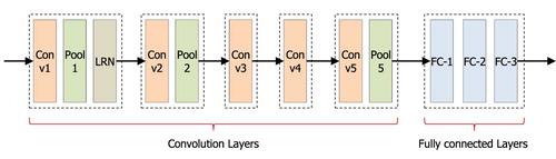
The five convolution layers have filter kernel sizes, strides, and output sizes indicated in the table below. Each convolutional layer uses the rectified linear unit (ReLU) as the non-linear activation function: (1) $\text{ReLU(}x\text{) = max}(0,x)$(1) Pool1, Pool2, and Pool5 are max-pooling layers after Conv1, Conv2, and Conv5 convolution layers respectively, and a local response normalisation (LRN) layer is added after Pool1 to locally normalise the feature map across neighbouring features, as expressed in Equation (2). (2) $b_{i,j,k}=\frac{a_{i,j,k}}{{\left[1+(\alpha /n){\sum }_{q=\text{max}(0,i-(n/2))}^{\text{min}(N-1,k+(n/2))}{(a_{i,j,k})}^2\right]}^{\beta }}$(2)

In the above equation, $a_{i,j,k}$ and $b_{i,j,k}$ represent the k-th feature map value at pixel location of the pooling output before and after normalisation, respectively. i is the output of the i th convolution kernel after using the activation function ReLU at position (x, y), N is the number of feature maps in the Pool1 output, q is the square cumulative index, which represents the sum of the squares of the pixel values q ∼ i, and $n,\alpha ,\beta$are hyper-parameters. In the experiments described in this paper, these values are used$n=5,\alpha =0.001,\beta =0.75$. The output feature map of each layer is a three-dimensional vector of shape, where C is the channel depth (number of features), H is the height of the feature map (number of rows), and W is the width of the feature map (number of columns). Table 1 shows the network parameters in VGG-S.

Table 1. VGG-S network parameters.

Layer name	Convolution kernel/ Stride/ Padding	Output size (C×H×W)
Data	—	3×256×256
Conv1	7×7/2/0	96×109×109
Pool1	3×3/3/0	96×37×37
LRN	—	96×37×37
Conv2	5×5/1/1	256×33×33
Pool2	2×2/2/0	256×17×17
Conv3	3×3/1/1	512×17×17
Conv4	3×3/1/1	512×17×17
Conv5	3×3/1/1	512×17×17
Pool5	3×3/1/1	512×6×6
FC-1		4096
FC-2		4096
FC-3		1000

2.2. Transfer learning

Transfer learning addresses the problem of insufficient training data required for deep learning (Tan et al., 2018). In transfer learning, model parameters are not trained from scratch; instead, they are “transferred” from a similar network pre-trained with another, usually much larger training dataset. The new model with the transferred parameters is then refined with the smaller, dedicated dataset. This approach can significantly reduce training time and the amount training data needed. Studies have shown that CNNs learned with transfer learning can achieve significant accuracy improvements in various applications (Tan et al., 2018). Usually, the first few layers of any CNN containing low-level edge and texture features which are suitable for most general machine vision tasks can be ported directly over amongst different machine vision tasks. The deeper layers, on the other hand, contain high-level semantic features which is specific to their respective tasks; so these are not re-usable between applications. The combination of porting low-level parameters and fine-tuning the higher-levels in transfer learning with a small training set avoids the problem of over-fitting neural networks due to the lack of sufficient training data, and has been proved as a useful strategy for different types of computer vision tasks with a small amount of training data available (Lima et al., 2017).

2.3. Auto-encoder

The basic auto-encoder (Bengio, 2009) is a three-layer unsupervised neural network structure which is divided into two halves – the encoder and the decoder. As shown in Figure 2, each auto-encoder (AE) has three layers of data – an input layer, a hidden layer and an output layer. The input and the output are represented as $x=[x_n]\in {\mathrm{\Re }}^N$ and $y=[y_n]\in {\mathrm{\Re }}^N$respectively, where N is the number of features per input and output sample. The hidden layer is the feature vector $h=[h_n]\in {\mathrm{\Re }}^H$, where H is the number of features of the hidden layer. Usually, $H<N$ in order for the auto-encoder to compress data, suppress noise or simplify data structure. In this paper, the number of features in the hidden layer is equal to the number of input and output features, that is, H = N.

Figure 2. Structure of an auto-encoder.

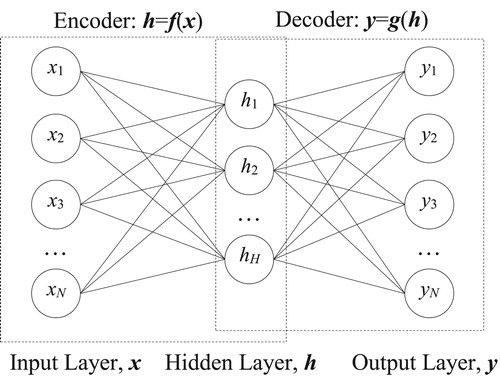
The encoding function and the decoding function are represented by f and g respectively. The encoding function is expressed as: (3) $\begin{array}{rl}{h}_{11}& =f_{{\theta }_{11}}(x)=s(W_{11}x+b_{11})\end{array}$(3) (4) $\begin{array}{rl}s(t)& =\frac{1}{1+e^{-t}}\end{array}$(4) where s(t) is the activation function of the encoder performed element-wise, $x$ is the feature vector of the convolutional layer, $f_{{\theta }_{11}}$ represents the encoding function, $W_{11}$ indicates the weight matrix between the input layer and the hidden layer, $b_{11}$ is the bias, and ${\theta }_{11}=\{W_{11},b_{11}\}$ means the connection weights and bias parameters between the input layer and the hidden layer. The decoder maps the hidden layer representation h to the output layer y through the decoding function: (5) $y=g_{\theta }(h)=s(W^{T}h+b)$(5)

The weight matrix representing the decoder is W^T, the transpose of the encoder weight matrix, while $b\in {\mathrm{\Re }}^N$ is the decoder’s bias. The aim of this auto-encoder is to find the parameters $\theta =\{\text{W},a,b\}$ which minimise the discrepancies between the inputs $x\in {\mathrm{\Re }}^N$ and the outputs $y\in {\mathrm{\Re }}^N$ whose difference is given as: (6) $J(x,y;\theta )=-\sum _{n=1}^N[x_n\log (y_n)+(1-x_n)\log (1-y_n)]$(6)

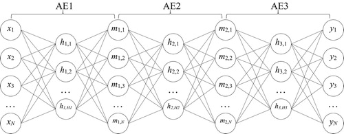
Auto-encoders can be concatenated one after another, where the outputs of the current auto-encoder are used as inputs of the next encoder. These concatenated structures are termed serial auto-encoders and can be used to extract features with progressive abstractions.

2.4. Serial auto-encoder

An auto-encoder consists of three layers (input, hidden, and output) connected by an encoder and a decoder. A series of auto-encoders can be concatenated back-to-back to form a serial auto-encoder, which the current auto-encoder shares its output layer with the next auto-encoder as input. Hence an M­­-length serial auto-encoder with input x and output y can be expressed as M auto-encoders. (7) $y=A{E}_M(\dots A{E}_2(A{E}_1(x;{\theta }_1);{\theta }_2)\dots ;{\theta }_M)$(7)

Alternatively, each j^th auto-encoder can be expressed as: (8) $m_j=A{E}_j(m_{j-1};{\theta }_j)$(8) where m_j is the output of the jth auto-encoder and m_j-1 is the input of the jth auto-encoder, which is also the output of the (j-1)th auto-encoder. Note that the M hidden layers h_j can have different sizes H_j while the input (m₀), output (m_M), and every middle layer (m_j, j=1, … , M-1) all have size N (Figure 3).

Figure 3. An example of 3-serial auto-encoder.

3. Proposed method

This paper proposes an adaptive weights-learning network model (AWL), which combines: (i) transfer learning of pre-trained VGG-S and feature extraction, and (ii) feature refinement with dual serial auto-encoders and adaptive feature weights, to perform image classification for CSI. The entire network is shown in Figure 4. Firstly, the VGG-S model is pre-trained with the ImageNet image dataset, and a refined VGG-S network model is obtained through transfer learning using CSI image dataset. Then, for each training sample, a convolution layer feature map and a fully connected layer features are extracted. A pair of AE network is then constructed separately, one trained with the convolution layer features and the other with the fully connected layer features. Finally, the obtained features are adaptively weighted, merged and the test samples are classified by using the trained network.

Figure 4. Adaptive weight learning network architecture.

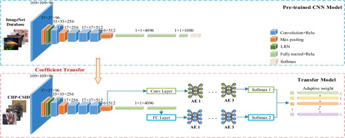
3.1. CNN transfer learning and feature extraction

A traditional CNN-based classifier passes its activations as a feature map from its last convolutional layer into a series of fully connected classifier layers. However, as different layers carry different aspects of the image information, every single layer of features on its own is insufficient to represent the image. Hence the combination of a few layers of features provides better representation (Xin et al., 2018). The low-level convolutional layers represent more primitive features such as edges, textures, contours and shapes. As we traverse deeper into the network, the resolution of the feature maps decreases while the amount of high-level semantic information increases (Li et al., 2018). Hence, we extract features from multiple layers of the neural network. The steps of the feature extraction based on transfer learning are as follows:

1. Initialise the VGG-S Model with parameters pre-trained with the ImageNet dataset.

2. Freeze the parameters of the 5 convolution layers, and continue to train the 3 fully connected layers using the CSI image dataset. The learning rate is set to 0.0005, and the number of iterations is limited to 40.

3. For each CSI dataset sample, extract the last pooled layer of the convolutional neural network model (Pool5) as a convolution layer features, F_conv.

4. For each CSI dataset sample, extract the second fully connected layer (FC-2) as the fully connected layer features, F_FC.

3.2. Adaptive weight learning

An important part of the AWL network model is a weight learning neural network module composed of auto-encoders and Softmax activations, and the process of adaptive weight learning based on feature maps from the convolution and fully connected layers generated by CSI Images. The steps of adaptive weight learning are summarised as follows:

1. Extract F_conv, the feature maps from the max-pool layer after the 5th convolutional layer and F_FC, the 2^nd fully connected layer of the final CNN model. Furthermore, F_conv is flattened and dimensionally reduced via a single auto-encoder to generate F′_conv which has the same shape as F_FC.

2. Build SAE_conv, a serial auto-encoder consisting of 1–3 auto-encoders followed by a fully connected classifier with the Softmax activation function. Input SAE_conv with F′_conv.

3. Build SAE_FC, a serial auto-encoder consisting of 1–3 auto-encoders followed by a fully connected classifier with the Softmax activation function. Input SAE_FC with F_FC.

4. Pass the CSI image dataset images into the post-trained VGG-S Net to extract the set F′_conv and F_FC. Use these feature map sets to train SAE_conv and SAE_FC respectively. Instead of using the trained weights of SAE_conv and SAE_FC for subsequent classification purposes, we obtain their corresponding aggregate classification losses generalised by the following expression for the next stage: (9) $J_{agg}(SAE)=-\frac{1}{M}\left[\sum _{m=1}^{M}J(x_m,y_m;\theta )\right]$(9) In the above equation, M represents the total number of samples in the training set, {x_m, y_m} is the inputs to the SAE and target classes respectively. J() is the loss function for individual sample. The two aggregate losses are termed as J_agg(SAE_conv) and J_agg(SAE_FC).

3.3. Feature fusion

In the above steps, the SAE model is trained with feature maps extracted from a convolutional layer and a fully connected layer, and the network parameters are fine-tuned to fully exploit the advantages of the convolutional layer and the fully connected layer which are representative of different levels of abstraction. The extracted features F_conv and F_FC both are normalised, and then feature fusion is used based on the aggregate training costs of SAE_conv and SAE_FC to form the final feature which is fed into a new classification layer whose inputs are F′_conv and F_FC: (10) $F_{fusion}=\frac{1}{J_{agg}(SA{E}_{CONV})}{F}_{CONV}^{\mathrm{\prime }}+\frac{1}{J_{agg}(SA{E}_{FC})}{F}_{FC}^{}$(10)

Better classification of CSI evidential images is then achieved when the fused features are used in the Softmax classifier.

4. Experiment results and analysis

4.1. Datasets and performance Indicators

4.1.1. Datasets

In order to verify the effectiveness of the proposed method on CSI image classification task and its applicability on other image datasets, the experiments used images from three different sources – the CSI image dataset and two public datasets The detailed description of each dataset is given in Table 2.

Table 2. Detailed description of the test datasets.

Name	Description	Class count	Image counts
CIIP-CSID1	bloodstains, vehicles, fingerprints, site plans, shoe prints, skin, tattoos, crime tools, windows, tire patterns	10	5000
CIIP-CSID2	biological evidence, bloodstains, vehicles, doors, fingerprints, site plans, shoe prints, skin, tattoos, crime tools, windows, tire patterns	12	9600
CIIP-CSID3	biological evidence, bloodstains, vehicles, doors, fingerprints, site plans, shoe prints, skin, tattoos, crime tools, windows, tire patterns	12	10600
GHIM-10K	sunsets, fireworks, architectures, cars, dragonflies, snow mountains, flowers, trees, fields, beaches, airplanes, butterflies, the Great Wall, Forbidden City, motorcycles, sailing boats, warships, chickens, insects, horses	20	10000
Corel-1K	Africa, beaches, buildings, buses, dinosaurs, elephants, flowers, horses, mountains, food	10	1000

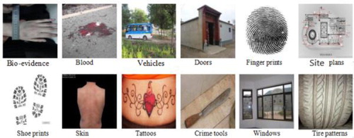
The CSI image dataset (CIIP-CSID) has been built by Center for Image and Information Processing (CIIP) in Xi'an University of Posts and Telecommunications (XUPT). It contains 19,363 actual CSI case images in 17 categories, such as biological evidence, vehicles, tire patterns, fingerprints, site plans, shoe prints, etc.

At present, there is no standard, publicly recognised large-scale image dataset in the field of CSI image research. References show that the CIIP-CSID dataset is the largest multi-class hybrid public CSI image dataset used by the academia. The images are all from real cases, and have been pre-processed according to the data confidentiality requirements from the police department. Figure 5 shows sample images in the CIIP-CSID dataset.

Figure 5. CIIP-CSID samples images.

In this experiment, three subsets CSI images of different scales are selected from CIIP-CSID dataset, namely CIIP-CSID1, CIIP-CSID2, and CIIP-CSID3. The CIIP-CSID1 dataset contains 5000 images in 10 categories, including bloodstains, vehicles, fingerprints, site plans, shoe prints, skins, tattoos, crime tools, windows, and tire patterns. The CIIP-CSID2 dataset contains 9600 images from 12 categories, such as biological evidence, bloodstains, vehicles, doors, fingerprints, and so on. The CIIP-CSID3 dataset contains images from the same 12 categories as in CIIP-CSID2, but at larger scale, with the total amount of images as 10600.

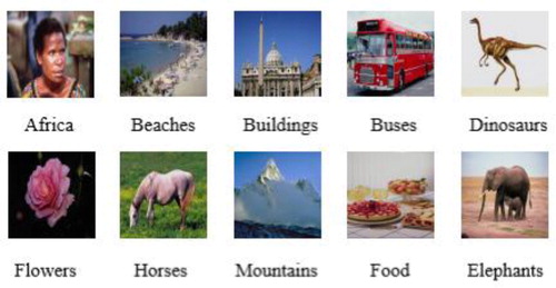
The public datasets GHIM-10 K and Corel-1 K are used to test the applicability of the proposed algorithm images with different contents. The GHIM-10 K dataset contains 10,000 natural images, divided into 20 categories such as sunsets, warships, flowers, architectures, cars, snow mountains, insects, and so on. The Corel-1 K dataset have 1000 images in 10 categories, including Africa, beaches, buildings, buses, dinosaurs, elephants, flowers, horses, mountains, and food. Figures 6 and 7 display sample images in GHIM-10 K and Corel-1 K, respectively.

Figure 6. GHIM-10 K samples images.

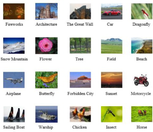
Figure 7. Corel-1 K samples images.

In the experiment part of this paper, 80% of the images in each category are selected as the training set and 20% as the test set. The experiments in this paper used MatConvNet to implement our algorithm. MatConvNet is a MATLAB toolbox that provides CNN function, many pre-trained CNN networks can be used. The experimental environment is Windows 10 operating system and the software programming environment is MATLAB R2016a.

4.1.2. Evaluation index

To evaluate the classification performance of the proposed algorithm, classification accuracy (Accuracy) and Average Accuracy (AA) are defined. (11) $\text{Accuracy}=\frac{T\text{i}}{N\text{i}}\times \text{100\%}$(11) (12) $AA=\frac{1}{N}\sum _{i=1}^N(\text{Accuracy}{)}_i$(12)

In the above formula, N_i is the total number of samples in class i, T_i is the number of correctly-classified samples in class i, and N is the total number of categories. The higher the accuracy measure, the better the classification. The Accuracy value represents the proportion of correctly classified images. The AA value indicates the average accuracy over all N classes.

4.2. Experimental results

Experiment 1: Comparison of classification performance between different network models and different network layers.

In order to validate the superiority of our proposed fine-tuned VGG-S network model, this experiment compares its classification accuracy with those of VGG-S, VGG-F, VGG-M, and AlexNet network models. The experimental results based on the CIIP-CSID3 dataset, Corel-1 K and GHIM-10 K datasets are shown in Table 3.

Table 3. Classification accuracy of different models in different databases.

	Accuracy (%)
Network model	CIIP-CSID3	Corel-1K	GHIM-10K
VGG-S	90.09	96.35	95.4
VGG-F	85.77	95.85	92.5
VGG-M	87.66	96.12	94.0
AlexNet	89.23	96.01	93.5
VGG-S-fine-tuned	91.83	95.65	96.0

As can be observed from the results in Table 3 above, different models have varying classification performance on the same image dataset. Taking the CIIP-CSID3 dataset as an example, the classification accuracy of the VGG-S model is 90.09%. The VGG-S-fine-tuned model has about 2% performance margin over the VGG-S model. At the same time, it is about 6% higher than the VGG-F model, and the performance is more prominent. In addition, comparing the classification accuracy of different network models on the public natural image datasets, our experimental results show that the VGG-S model performs best for classification on the Corel-1 K dataset. The classification accuracy of VGG-S model on Corel-1 K dataset is 96.35%, which is higher than 95.65% of VGG-S-fine-tuned model. The experimental results on the GHIM-10k dataset show that the classification accuracy of VGG-S – fine-tuned model is the highest, which can reach 96.0%, and is about 1% and 5% higher than that of VGG-S model and VGG-F model respectively. The experimental results show that since the Corel-1K dataset has small number of image categories and small amount of data, the VGG-S model has higher classification accuracy than the VGG-S-fine-tuned model. However, in the CIIP-CSID3 and GHIM-10K datasets which have lager training samples, the VGG-S-fine-tuned model performs better than the VGG-S model. In general, the VGG-S-fine-tuned model can give better results in the datasets with large amounts of data.

Experiment 2: Comparison of classification results of SAEs with different depths in various datasets.

In order to validate that AEs with various depths have different classification results, we compare the classification results of Serial AEs of different depths. The experimental results based on the CIIP-CSID1, CIIP-CSID2, CIIP-CSID3, Corel-1 K and GHIM-10 K datasets are shown in Table 4.

Table 4. Classification results of serial AEs of different depths.

Dataset	AE1 Iteration (Times)	AE2 Iteration (Times)	AE3 Iteration (Times)	Softmax Iteration (Times)	Fine-tuned Iteration (Times)	AA (%)
CIIP-CSID1	50	–	–	100	–	94.86
	50	50	–	100	–	94.88
	50	50	50	100	–	95.02
	50	50	50	100	100	95.21
CIIP-CSID2	50	–	–	100	–	95.11
	50	50	–	100	–	95.45
	50	50	50	100	–	96.03
	50	50	50	100	100	96.33
CIIP-CSID3	50	–	–	100	–	96.01
	50	50	–	100	–	96.82
	50	50	50	100	–	97.12
	50	50	50	100	100	97.41
GHIM-10K	50	–	–	100	–	98.32
	50	50	–	100	–	99.26
	50	50	50	100	–	98.33
	50	50	50	100	100	98.63
Corel-1K	50	–	–	100	–	99.89
	50	50	–	100	–	99.99
	50	50	50	100	–	99.99
	50	50	50	100	100	100

Table 4 records classification performances of AEs with different depths in various datasets. AEs in Table 4 represent the number of hidden layer features. 50/100 is the number of iterations. Results show that, the fine-tuned three-layer SAE has the best performance on the CIIP-CSID1, CIIP-CSID2, CIIP-CSID3 and Corel-1 K datasets, reaching 95.21%, 96.33%, 97.41%, 100% respectively. As for the results on the GHIM-10 K dataset, the average classification accuracy of the two-layer SAE is the highest, which is up to 99.26%, and has about 0.6% performance margin over the fine-tuned three-layer SAE. It can be seen that when there are many categories of datasets, it is not necessary to use multi-layer encoder to achieve good classification results. It can be seen from Table 4 that when the depths of the AEs vary, the classification results in the respective datasets also differ. The trainings with CSI images of different cardinalities yield different results. From the experimental results, it can be seen that when the training samples get larger, the classification effect will get better. In addition, we conclude from the classification results that the classification performance of the fine-tuned three-layer SAE is the best. However, since the GHIM-10 K dataset has the largest image category, it shows the best classification in the two-layer Serial AE. The Corel-1 K dataset has the highest average classification accuracy because of its small number of image categories and small amount of data. Therefore, depending on the dataset, its settings for the Serial AE should also be adjusted.

Experiment 3: Comparison of classification results of different features in CIIP-CSID3 datasets.

In order to compare the classification performance of different CNN features on the CSI images, we select the CIIP-CSID3 dataset and test the classification accuracy by using the convolution layer feature in CNN (Conv5), the fully connected layer feature in CNN (FC7), the fusion feature of convolution layer feature and fully connected layer feature in CNN (Conv5+FC7), CNN feature (CNN) and the AWL weight fusion method proposed in this paper. The results are displayed in Figure 8.

Figure 8. Classification results of different features on CIIP-CSID3.

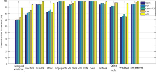
The results in Figure 8 tells that the proposed method improves the classification accuracy on the CSI image dataset, especially in “biological evidence”, “bloodstains”, “doors”, and “windows” classes, whereby the classification accuracies have increased between 10% and 20%. In addition, the classification accuracies of “site plans”, “tattoos”, “crime tools”, and “tire patterns” have increased by 1%-5% only. It is observed that for classes with lower within-class similarity (in other words, the content difference between images within the class is greater) such as biological evidence and windows, the proposed method brings more obvious performance improvement compared with other features. However, for classes with higher within-class similarity such as tire patterns, all the tested features seem to work well and the performance gain produced by the proposed method is little.

4.3. Discussion

The above three experiments have proved the effectiveness of the proposed algorithm. The first experiment compared the classification performance between different network models and different network layers. The results demonstrated that the classification performance of VGG-S-fine-tuned model performs the best. The second experiment compared the classification results of Serial AEs of different depths in different datasets. It is shown that when the depths of the AEs vary, the classification results in the respective datasets also differ. The third experiment compared the classification results of different features on the CIIP-CSID3 dataset. The results showed that the AWL feature fusion method proposed outperforms other features.

Attention mechanism imitates human visual behaviour and can find the salient region of an image. Therefore, researchers have introduced attention mechanism into CNN to extract image features with more powerful representation ability (Wang et al., 2017; Zhu et al., 2019). Our future work intends to leverage on attention mechanism to further improve the performance of CSI image classification. In (Wu, & Gao, 2018), the authors presented a fully convolutional network (FCN)-based model to implement pixel-wise classifications for remote sensing image, and an adaptive threshold algorithm is adopted to adjust the threshold of Jaccard index in each class. The adaptive threshold methodology could be further explored to enhance the performance of CSI image classification.

In practical application scenarios, some CSI images have complex and cluttered background, whilst the objects-of-interest can be partially occluded or occupy small portions of the images. These problems make the process of image feature extraction and the recognition of similar small targets difficult. In (Srivastava & Biswas, 2020), a learning method based on salient features is adopted. Only specific features are embedded in SVM classifier for deep feature extraction, which can achieve better classification accuracy and reduce the amount of calculation. In (Qian et al., 2020), a new feature detection method is proposed, which can extract rich semantic information from the edge and corner features of the target, and help to increase the number of effective feature points extracted from the image. These two feature extraction methods are worth trying in our future research. In (Zhu et al., 2020), the authors proposed a modified region-based fully convolutional network, which can identify out different leaves with similar characteristics in one scene. This method can be used to identify small targets such as shoe prints and fingerprints in CSI images, which is conducive to case analysis and comparison.

5. Conclusion

In this paper, a novel CSI image classification method has been proposed based on adaptive weighted fusion of multiple CNN feature layers. The method involves using transfer learning to extract the multi-layer CNN features for CSI images. It also involves constructing two serial auto-encoder networks for the multi-layer CNN features to obtain adaptive fusion weights through network training and parameter fine-tuning. The experimental results demonstrated the effectiveness of the proposed method on CSI image classification, as well as its applicability on other image data of different content.

Disclosure statement

No potential conflict of interest was reported by the author(s).

Correction Statement

This article has been republished with minor changes. These changes do not impact the academic content of the article.

Additional information

Funding

This work has been partially supported by National Natural Science Foundation of China [grant numbers 61802305, 61671377].

References

- Bai, X., Liu, Y., & Shen, Y. (2018). Application of deep learning in image classification of crime scene investigation. Journal of Xi'an University of Posts and Telecommunications, 23(5), 47–51. DOI:10.13682/j.issn.2095-6533.2018.05.007
- Bai, X., Shi, T. Y., & Liu, Y. (2016). An improved criminal scene investigation image classification algorithm. Journal of Xi'an University of Posts and Telecommunications, 21(6), 24–28. DOI:10.13682/j.issn.2095-6533.2016.06.005
- Bengio, Y. (2009). Learning deep architectures for AI. Foundations and Trends in Machine Learning, 2(1), 1–127. https://doi.org/10.1561/2200000006
- Bulan, O., Bernal, E. A., Loce, R. P., & Wu, W. C. (2012). Tire classification from still images and video. 2012 15th International IEEE Conference on Intelligent Transportation Systems (ITSC), 485-490.
- Chatfield, K., Simonyan, K., Vedaldi, A., Zisserman, A. (2014). Return of the devil in the details: delving deep into convolutional nets. Proceedings of the British Machine Vision Conference. United Kingdom: Springer, pp.1–12.
- Ezeobiejesi, J., & Bhanu, B. (2018). Latent fingerprint image quality assessment using deep learning. 2018 IEEE/CVF Conference on Computer Vision and Pattern Recognition Workshops (CVPRW), IEEE Computer Society, pp. 621-630.
- Krizhevsky, A., Sutskever, I., & Hinton, G. (2012). ImageNet classification with deep convolutional neural networks. NIPS, 25.
- Lan, R., Guo, S., & Jia, S. (2018). Forensic image retrieval algorithm based on fusion. Computer Engineering and Design, 39(4), 1106–1110. DOI:10.16208/j.issn1000-7024.2018.04.036
- Li, J., Zhou, X., Chan, S., Chen, S. (2018). A novel video target tracking method based on adaptive convolutional neural network feature. Journal of Computer-Aided Design & Computer Graphics, 30(2), 273–281. https://doi.org/10.3724/SP.J.1089.2018.16268
- Li, S., Zhu, X., Liu, Y., Bao, J. (2019). Adaptive spatial-spectral feature learning for hyperspectral image classification. IEEE Access, 7, 61534–61547. https://doi.org/10.1109/ACCESS.2019.2916095
- Lima, E., Xin, S., Dong, J., Hui, W, Yang, Y, Liu, L. (2017). Learning and transferring convolutional neural network knowledge to ocean front recognition. IEEE Geoscience and Remote Sensing Letters, 14(3), 354–358. https://doi.org/10.1109/LGRS.2016.2643000
- Liu, Y., Hu, D., Fan, J., Wang, F., Zhang, D. (2017). Multi-feature fusion for crime scene investigation image retrieval. 2017 International Conference on Digital Image Computing: Techniques and Applications (DICTA), IEEE, pp. 1–7.
- Liu, Y., Hu, D., & Fan, J. (2018). A survey of crime scene investigation image retrieval. Chinese Journal of Electronics, 46(3), 761–768. DOI:10.3969/j.issn.0372-2112.2018.03.035
- Liu, Y., Liu, Q., Fan, J., et al. (2020). Tyre pattern image retrieval – current status and challenges. Connection Science. DOI:10.1080/09540091.2020.1806207
- Liu, Y., Peng, Y., Lim, K., Ling, N. (2019). A novel image retrieval algorithm based on transfer learning and fusion features. World Wide Web, 22(3), 1313–1324. https://doi.org/10.1007/s11280-018-0585-y
- Liu, Y., Wang, F., Hu, D., et al. (2017). Multi-feature fusion with SVM classification for crime scene investigation image retrieval. IEEE International Conference on Signal & image Processing. IEEE, 160–165. DOI:10.1109/SIPROCESS.2017.8124525.
- Liu, Y., Zhang, S., Wang, F., & Ling, N. (2018). Read pattern image classification using convolutional neural network based on transfer learning. IEEE Workshop on Signal Processing Systems (SIPS, 2018), pp. 21–24.
- Qian, J., Zhao, R., Wei, J., Luo, X., Xue, Y.,(2020). Feature extraction method based on point pair hierarchical clustering. Connection Science, 32(3), 223–238. DOI:10.1080/09540091.2019.1674246.
- Srivastava, V., & Biswas, B. (2020). CNN-based salient features in HSI image semantic target prediction. Connection Science, 32(2), 113–131. https://doi.org/10.1080/09540091.2019.1650330
- Tan, C., Sun, F., Kong, T., et al. (2018). A survey on deep transfer learning. International Conference on Artificial Neural Networks (ICANN, 2018), pp. 270–279.
- Vagac, M., Povinsky, M., & Melichercik, M. (2017). Detection of Shoe Sole Features Using DNN, 2017), IEEE 14th International Scientific Conference on Informatics, IEEE, pp. 416–419.
- Wang, F., Jiang, M., Qian, C., et al. (2017). Residual attention network for image classification. Computer Vision and Pattern Recognition, 6450–6458. DOI:10.1109/CVPR.2017.683.
- Wu, Z., Gao, Y., Li, L., Xue, J., Li, Y. (2018). Semantic segmentation of high-resolution remote sensing images using fully convolutional network with adaptive threshold. Connection Science, 31(2), 169–184. https://doi.org/10.1080/09540091.2018.1510902
- Xin, P., Xu, Y., Tang, H., et al. (2018). Fast airplane detection based on multi-layer feature fusion of fully convolutional networks. Acta Optica Sinica, 38(3), 344–350. DOI:10.3788/AOS201838.0315003.
- Xu, Z., & Zhang, W. (2020). Hand segmentation pipeline from depth map: An integrated approach of histogram threshold selection and shallow CNN classification. Connection Science, 32(2), 162–173. https://doi.org/10.1080/09540091.2019.1670621
- Zhao, Y., Wang, Q., & Fan, J. (2014). Fuzzy KNN classification for criminal investigation image scene. Applications Research of Computers, 31(10), 3158–3160. DOI:10.3969/j.issn.1001-3695.2014.10.067.
- Zhu, X., Cheng, D., Zhang, Z., et al. (2019). An Empirical Study of Spatial Attention Mechanisms in Deep Networks, 2019), IEEE/CVF International Conference on Computer Vision (ICCV), Seoul, Korea (South), 6687-6696.
- Zhu, X., Zuo, J., & Ren, H. (2020). A modified deep neural network enables identification of foliage under complex background. Connection Science, 32(1), 1–15. https://doi.org/10.1080/09540091.2019.1609420