Deep blur detection network with boundary-aware multi-scale features

Abstract

Recently, blur detection is a hot topic in computer vision. It can accurately segment the blurred areas from an image, which is conducive for the post-processing of the image. Although many hand-crafted features based approaches have been presented during the last decades, they were not robust to the complex scenarios. To solve this problem, we newly establish a boundary-aware multi-scale deep network in this paper. First, the VGG-16 network is used to extract the deep features from multi-scale layers. Contrast layers and deconvolutional layers are added to make the difference between the blurred areas and clear areas more prominent. At last, a new boundary-aware penalty is introduced, which makes the edges of our results much clearer. Our method spends about 0.2 s to evaluate an image. Experiments on the large dataset confirm that the proposed model performs better than other models.

Keywords:

• Blur detection
• multi-scale
• boundary-aware
• deep learning

1. Introduction

Blur detection without any knowledge about the blur type, level and the camera setting is a challenging problem. It aims to accurately segment the blurred areas in an image. It is very useful in many interesting applications, such as image restoration (Zhang et al., 2016), defocus magnification (Bae & Durand, 2007), salient object detection (Jiang et al., 2013; Sun et al., 2017), blur segmentation and deblurring (Shi et al., 2014, 2015), and so on. Blur detection is different from the object detection. It aims to detect the blurred parts of an image, not only the objects. According to the cause of blurness, the blur could be divided into out-of-focus (Figure 1(a)) or motion blur (Figure 1(b,c)).

Figure 1. Some examples of different blur detection tasks. In the sub-figure, the left is the original image and the right is its ground truth for blur detection. The white masks denote the blurred regions. (a) Example of the clear object and blurred background. (b) Example of a blurred object and (c) Example of blurred regions.

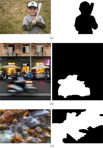
As shown in Figure 1, the blurred parts of an image could be an object, or a region, even the rest parts of an image excluding the clear object. In the case of Figure 1(a), since there is a clear object and the blurred regions are almost the whole background, it is easier to get a good detection result benefiting from some skills of object detection. But in the case of Figure 1(b,c), things are more difficult because the blurred regions are no longer limited to the background. The uncertainty and diversity of the blurred regions make the blur detection task more challenging to the traditional detection tasks.

Sometimes, the blur is purposely generated by photographers. They take a wide aperture and prevent light converging to achieve a visual effect, which makes the important objects more prominent. This photography skill is very common in the images captured by optical imaging systems. Based on studying the cause of blurness, many methods were proposed to solve this problem. In Levin (2007), they tried to identify partial motion blur via analysing the statistics information of an image. In Liu et al. (2008), they used four local blur features to detect the blurred regions. In Chakrabarti et al. (2010), they first used the local Fourier transform to solve this problem. In Shi et al. (2014), they analysed the discriminative features for the blur detection task in gradient and Fourier space. All these methods belong to the hand-crafted features based methods. In simple scenarios, they are convenient and often effective; however, they cannot handle the complex scenarios well.

One possible reason is that it is hard to segment the blurred areas from the smooth areas inside a clear object. There is no structural information in blurred areas, including clear boundaries and textures. Neither does the smooth areas inside a clear object. Only depending on the low-level cues, it is too hard to distinguish them. The second reason is that the traditional methods are more sensitive to the edges of objects, but they often fail when there is not a clear object in an image, just as the case of Figure 1(b,c). For these two possible reasons, in this paper, we avoid to design a new hand-crafted feature. Instead, we set up a multi-scale deep network to learn which regions are blurred in an arbitrary image.

During the last five years, convolutional neural network (CNN) has developed very fast. It has performed better than the traditional methods in many applications, including object detection (Kang et al., 2016; Srivastava & Biswas, 2020; Xu & Zhang, 2020; Zhu et al., 2020), image classification (Wei et al., 2015), image denoising (Zhang, K. et al., 2017), image super-resolution (Dong et al., 2015), saliency detection (Zhang, P. et al., 2017), object tracking (Sun et al., 2018) and network optimisation (Liu et al., 2020; Wang et al., 2016; Xue & Wang, 2015, 2016; Ye et al., 2016). Inspired by these facts, we proposed a boundary-aware multi-scale deep network to solve the blur detection problem in this paper. First, the image scales are one of the most important factors to determine the blur confidence of an image (Shi et al., 2014). Motivated by this observation, we used the VGG-16 network (Simonyan & Zisserman, 2015) to get the feature maps with different scales from an input image. Second, we used a series of contrast layers to strengthen the differences between the blurred areas and the clear areas. And we connected the corresponding deconvolution layers to get the final estimation result with the same resolution of input image. Finally, a new loss function was added to force the blur boundary more clear. Since our new model is not based on the image patches, it is trained end-to-end. Our new model spends only 0.2 s evaluating an input image. Experiments on the large dataset show that the performance of our new model is better than the other methods.

In a word, our contributions in this paper are summarised as follows:

• We have given an deep blur detection network which has achieved a good balance between fast running speed and high detection accuracy. Our network architecture is simple, clear and effective.

• We have demonstrated it is more useful to use the contrast layers as the skip connection between the encoder network and the decoder network. It could be also useful for the other applications base on the contrast features, such as salient object detection, etc.

• We proposed a boundary-aware loss function, which penalised the errors on the boundary. Benefiting from the new loss function, our blur detection results have more clear edges and much cleaner background.

The rest sections are arranged as follows. Section 2 summarises the related literatures. The proposed model is detailed described in Section 3. In Section 4, we have shown a plenty of experiments and the comparison results. At last, we give the conclusion in Section 5.

2. Related work

Traditional blur detection models include two categories: the gradient magnitude-based methods (Chen et al., 2020; Elder & Zucker, 1998; Su et al., 2011; Tai & Brown, 2009, etc.) and frequency space-based methods (Golestaneh & Karam, 2017; Lu et al., 2016; Shi et al., 2014; Tang et al., 2016; Wu et al., 2019, etc.).

It is observed that if an image patch is clear, there are more strong gradients. Based on this observation, in Elder and Zucker (1998), and Tai and Brown (2009), the authors used the ratio of strong gradient magnitude to characterise the sharpness of an image patch. In Su et al. (2011), the authors combined the distributions of singular value and gradient pattern in the alpha channel, which was used to detection the blur areas.

In frequency space, a blur image often has less high-frequency components and more low-frequency components. Based on this fact, many methods were proposed in frequency space. They detected the blur areas by calculating the ratio of high-frequency components for an given image. In Golestaneh and Karam (2017), the authors combined the multi-scale blur detection maps in high frequency. In Shi et al. (2014), the authors have proposed four effective descriptors including a Fourier domain descriptor. In Tang et al. (2016), the authors iteratively refined the coarse blur map by using the similar neighbour image patches. In Lu et al. (2016), the authors used unsigned utility magnitudes to compute the blur areas.

In some simple scenarios, the hand-crafted features have shown good performance, but they often fail in the complex scenes, just as shown in Figure 1(b,c). The blur detection task is still an open problem.

3. Boundary-aware multi-scale deep network for blur detection

3.1. Network architecture

In this paper, we propose an end-to-end fully convolutional and boundary-aware multi-scale network to segment the blur areas from an given image. The entire network of our model is shown in Figure 2. As shown, the entire network contains five scales and three rows. Five scales mean to extract the features with multi-resolutions. Three rows are used for feature extracting, contrast computation and up-sampling processing, respectively. The input image I is resized to $352\times 352$. The estimated blur map is $176\times 176$, and we resize it back to $352\times 352$ with a bilinear interpolation. The detailed network settings are listed in Table 1.

Figure 2. The entire network architecture of our model.

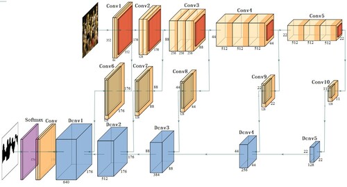
Table 1. Details of our boundary-aware multi-scale deep network for estimating the blur maps.

Layer	Contents	Kernel	Stride	Resolution	Channels
Conv1	Conv*2	3*3	1	352*352	64
	Max-pool	2*2	2	176*176	64
Conv2	Conv*2	3*3	1	176*176	128
	Max-pool	2*2	2	88*88	128
Conv3	Conv*3	3*3	1	88*88	256
	Max-pool	2*2	2	44*44	256
Conv4	Conv*3	3*3	1	44*44	512
	Max-pool	2*2	2	22*22	512
Conv5	Conv*3	3*3	1	22*22	512
	Max-pool	2*2	2	11*11	512
Conv6	Conv	3*3	1	176*176	128
	Diff	3*3	1	176*176	128
Conv7	Conv	3*3	1	88*88	128
	Diff	3*3	1	88*88	128
Conv8	Conv	3*3	1	44*44	128
	Diff	3*3	1	44*44	128
Conv9	Conv	3*3	1	22*22	128
	Diff	3*3	1	22*22	128
Conv10	Conv	3*3	1	11*11	128
	Diff	3*3	1	11*11	128
Dcnv1	Deconv	5*5	2	176*176	640
Dcnv2	Deconv	5*5	2	176*176	512
Dcnv3	Deconv	5*5	2	88*88	384
Dcnv4	Deconv	5*5	2	44*44	256
Dcnv5	Deconv	5*5	2	22*22	128
Conv	Conv*2	1*1	1	176*176	2
Softmax	Softmax	1*1	1	176*176	2

As mentioned in Section 1, the multi-scale resolutions are important to the blur detection task. In our network, the first row includes five layers coming from VGG-16 network (Simonyan & Zisserman, 2015). All of these five layers connect with a max-pooling layer, which down-samples $\{F_1,F_2,\dots ,F_5\}$ by a stride of 2. The output resolutions of these five layers are $\{176\times 176,88\times 88,\dots ,11\times 11\}$, respectively.

The second row contains five layers, named Conv6 to Conv10, which are connected to the Conv1 to Conv5, respectively. These five layers aim to compute the contrast features $\{C_1,C_2,\dots ,C_5\}$. These contrast features are local, which capture the lost of object details compared to their local neighbourhoods.

The last row contains five deconvolution layers, which fuse and up-sample the feature maps from the first row and the contrast feature maps from the second row. The up-sample factor is 2, therefore, the resolution changes from $11\times 11$ to $176\times 176$ step by step. The final estimated blur map is got after two convolution layers and one softmax operation.

3.2. Multi-scale features extraction

The multi-scale perception in blur detection has been noticed in Shi et al. (2014). Looking from one singe resolution, it is hard to accurately identify whether an area of an image is blur. Looking from the large scale, an image may be clear, but when looking into the smaller scale, if no more details of structures or textures information provided, it is considered to be blurred. That is called the scale ambiguity (Lu et al., 2013; Yan et al., 2013).

In this paper, we use VGG-16 network (Simonyan & Zisserman, 2015) as our pre-trained network. It has multiple stages of spatial pooling, which progressively down-sample the input image, resulting in a multi-resolutions feature maps. To transform the original VGG-16 model into a fully convolutional network, we only reserve the first five down pooling blocks of VGG-16 network as the multi-scale feature extraction layers, e.g. Conv1 to Conv5, and the multi-resolutions feature maps are denoted as $\{F_1,F_2,\dots ,F_5\}$.

3.3. Skip connection using contrast layers

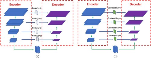
Skip connection has been recently used to associate the low-level features maps across resolutions. For example, it was used in U-Net (Milletari et al., 2016) and SharpMask (Pinheiro et al., 2016) for segmentation, in Recombinator networks (Honari et al., 2016) for face detection, and in Stacked Hourglass networks (Newell et al., 2016) for keypoint estimation. The skip connection was often executed by a convolutional layer with $1\times 1$ resolution, named Conv(1*1), just as shown in Figure 3(a). In this paper, we used a contrast layer as the skip connection instead of Conv(1*1), as shown in Figure 3(b), because we found that it was more effective to strengthen the contrast features between the blur regions and the clear regions than only to introduce them.

Contrast features are often used in salient object detection (Achanta et al., 2009; Jiang et al., 2013; Yan et al., 2013). In blur detection task, the clear image refers to the image with clear edges, subtle textures, and rich detailed information. On the other hand, the blurred image has blurred edges or textures, and is often lack of details. Therefore, the contrast features are also useful in blur detection. But the contrast features for blur detection are more difficult to extract. In the past, the contrast features for blur detection are founded through image statistics information in gradient distribution (Jiang et al., 2013; Liu et al., 2008; Su et al., 2011; Zhao et al., 2013; Zhuo & Sim, 2011) or in frequency space (Park et al., 2017; Shi et al., 2014; Tang et al., 2013, 2016; Vu et al., 2011). Instead of finding a new hand-crafted features, in this paper, we use a series of local contrast features layers to capture the difference between clear and blurred regions.

Figure 3. Skip connection using contrast layers. (a) Skip connection using Conv(1*1), (b) Skip connection using Contrast Layers.

We connect a convolutional layer to each scale feature map, e.g. Conv6 to Conv10. Each convolutional layer has a kernel size $3\times 3$ and 128 channels. And each contrast feature map $C_i$ is calculated as follows: (1) $C_i=\mathrm{D}\mathrm{i}\mathrm{f}\mathrm{f}\left(F_i\right)=F_i-\mathrm{A}\mathrm{v}\mathrm{g}\mathrm{P}\mathrm{o}\mathrm{o}\mathrm{l}\left(F_i\right)$(1) Note our contrast features are learned and not pre-defined. The size of each contrast feature map $C_i$ is equal to the corresponding feature map $F_i$.

3.4. Deconvolution layers

Since we have got a lot of contrast feature maps from different scales, we need a fuse category to fuse them together and generate the final estimated blur map with the same size of input image. We adopt five deconvolution layers each connected to one contrast layer. In the same time, the lower deconvolution layer is connected to the higher deconvolution layer. The feature map is up-sampled from the lowest deconvolution layer to the highest by a factor of 2 one layer after another. At each deconvolution layer, the resulting up-pooled feature map $U_i$ is computed by combining the corresponding contrast feature map $C_i$ and the previous up-pooled feature map $U_{i+1}$. It is defined as follows: (2) $U_i=\mathrm{U}\mathrm{p}\mathrm{P}\mathrm{o}\mathrm{o}\mathrm{l}(C_i,U_{i+1})$(2) The final estimated blur map is the result of $U_1$ after two convolutional layers and one softmax layer. The detailed network parameters could be found in Table 1.

3.5. Boundary-aware loss function

Given the training set $\{\mathrm{\Omega }=(U,G\left)\right\}$, where U denotes the estimated blur maps, and the G denotes the ground truths. Here, x, y denotes the coordinate of one pixel. The pixel-wise loss function between the estimated blur maps U and the ground truths G is generally defined as follows: (3) $L\left(\mathrm{\Theta }\right)=-\sum _{\mathrm{\Omega }}\sum _{x,y}\{G_{x,y}\log \rho (U_{x,y}|\mathrm{\Theta })+(1-G_{x,y})\log (1-\rho (U_{x,y}|\mathrm{\Theta }\left)\right)\}$(3) where (4) $\rho \left(U_{x,y}|\mathrm{\Theta }\right)=(1+e^{-U_{x,y}}{)}^{-1}$(4) Here, Θ denotes the parameter set.

Motivated by the progress on medical image segmentation (Milletari et al., 2016; Taha & Hanbury, 2015; Zou et al., 2004), in this paper, we use a boundary-aware loss function to approximate the penalty on boundary length. To compute the boundary pixels, we use a Sobel operator and a tanh function to get the gradient magnitude in the estimated blur map. The tanh function could project the gradient magnitude of the estimated blur map to a probability range of $[0,1]$. The boundary penalty term is defined as follows: (5) $L_{Boundary}=1-\frac{\left|{\hat{U}}_i\cap {\hat{G}}_i\right|}{\left|{\hat{U}}_i\cup {\hat{G}}_i\right|}$(5) where ${\hat{U}}_i$ denotes the gradient magnitude of the results, and ${\hat{G}}_i$ denotes the corresponding ground truth.

The final loss function of our model is the sum of Equations (3(3) $L\left(\mathrm{\Theta }\right)=-\sum _{\mathrm{\Omega }}\sum _{x,y}\{G_{x,y}\log \rho (U_{x,y}|\mathrm{\Theta })+(1-G_{x,y})\log (1-\rho (U_{x,y}|\mathrm{\Theta }\left)\right)\}$(3) ) and (5(5) $L_{Boundary}=1-\frac{\left|{\hat{U}}_i\cap {\hat{G}}_i\right|}{\left|{\hat{U}}_i\cup {\hat{G}}_i\right|}$(5) ). This final loss function is boundary penalised and the computation procedure is end-to-end trainable. Its usage will be demonstrated in the experimental section.

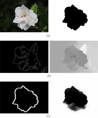
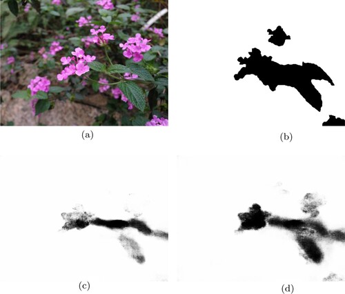
Here, we have shown the comparison with the other methods using gradient magnitude in Figure 4. In Figure 4(a), there is an original image and the corresponding ground truth. In the Figure 4(b), the left is the gradient magnitude detected by a Sobel edge detector in Zhuo and Sim (2011), and then the blur amount at edge locations was the propagated to the entire image to get the final blur map in the right. In Figure 4(c), the left is the learned boundary by our method after 200 epochs of training process, the right is our detected blur map. Obviously, the learned boundary after 200 cycles are more accurate to the boundary of ground truth. This will be useful for a better blur map.

Figure 4. Comparison with the other methods using gradient magnitude. In (a), the left is original image and the right is the ground truth; in (b), the left is the gradient magnitude and the right is the result generated by Zhuo and Sim (2011); in (c), the left is the our learned boundary and the right is the result of our method. (a) Image and GT. (b) Zhuo and Sim (2011) and (c) Our method.

4. Experiments

4.1. Experimental setup

4.1.1. Dataset

The blur detection dataset proposed in Shi et al. (2014) is selected as the evaluating dataset. For the convenience, this blur detection dataset is named Shi's dataset¹ in this paper. As far as we know, it is the largest public blur detection dataset with pixel-wise ground truths. It contains 1000 images with pixel-wise ground truth annotations for the blurred regions. Ground truth masks are produced by 10 volunteers. It varies a lot in contents, including images with defocus blur or motion blur.

4.1.2. Experimental setup

Our blur detection model was based on TensorFlow (Abadi et al., 2016) platform. The weights in the Conv1 to Conv5 layers were initialised with the pre-trained weights of VGG-16 network (Simonyan & Zisserman, 2015). All the weights of new layers were randomly initialised with a truncated normal distribution ($\delta =0.01$). The Adam optimizer (Kingma & Ba, 2015) is adopted in our training process. Initial learning rate is set to ${10}^{-6}$.

For avoiding over-fitting problem, we selected the first 500 images from the Shi's dataset as our training set, and used the following 100 images as the validation set. The rest 400 images are used to test. The images of training dataset were resized to $352\times 352$.

Our model was trained on a personal computer. The CPU is an Intel i7-8750H, and the memory is 8GB. The Nvidia GeForce GTX1060 GPU is used in our computer. It spent about 12 h for 20 epochs during the training stage, and we needed only 0.2 s to generate the estimated blur map for a testing image with $352\times 352$ resolution.

4.1.3. Evaluation metrics

In the experiments, six metrics (Ma et al., 2018) are selected as the metrics, including the precision-recall curves, average of Precision values, average of Recall values, mean absolute error, the max F-measure score and the structural measures. For convenience, they are abbreviated as PR curves, Avg(Precision), Avg(Recall), MAE, Max-F and S-measure, respectively.

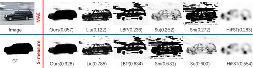
To more easily understand how to use different metrics to evaluate different methods, in Figure 5, we have given an illustration. In this figure, given an input image and the corresponding ground truth (GT), the results of 6 methods are shown and two metrics (MAE and S-measure) are used to evaluate their performances. As shown in the first row, since the MAE value is the smaller the better, we have sorted the performances of 6 methods from left to right. But the S-measure value is the bigger the better, as shown in the second row, we still arrange the best method to the most left. According to the MAE,  Su et al. (2011) method is better than  Shi et al. (2014) method, but according to the S-measure,  Shi et al. (2014) method is better. Therefore, by evaluating the performance from different views, we could give a comprehensive comparison to all these methods. Taking Figure 5 as an example, we can see that our method achieves the highest value of S-measure and the lowest value of MAE, so the comprehensive performance of our method is best.

Figure 5. Different evaluation views in terms of MAE and S-measure.

4.2. Ablation studies

4.2.1. Effectiveness of the boundary penalty

To demonstrate the effectiveness of our newly added boundary penalty to the loss function, we removed the boundary penalty from our model and the rest parts remained the same. Then we trained the “ours_1” network for 20 epochs and the quantitative results were reported in the Table 2. Using MAE value, our newly added boundary penalty has improved our method by about 8% on Shi's dataset. In the Figure 6, we have shown the comparison of results generated from our model without and with boundary penalty. Result with boundary penalty is more clear at the object boundaries, and the background is also cleaner.

Figure 6. Comparison of results generated from our model without and with boundary penalty. (a) Original Image. (b) GT. (c) Result without boundary penalty MAE = 0.097 S-measure = 0.885 and (d) Result with boundary penalty MAE = 0.033 S-measure = 0.943.

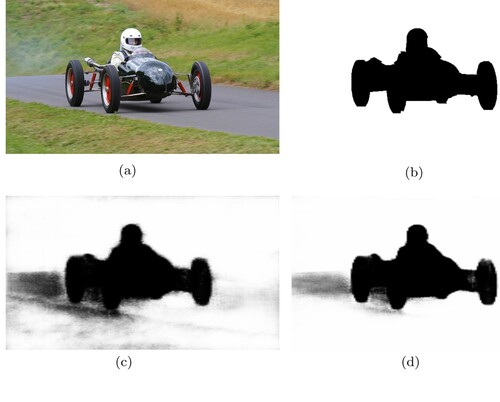
Table 2. Model analysis results.

Metrics	Ours_1^a	Ours_2	Ours
MAE↓	0.227	0.221	0.210
Max-F↑	0.750	0.753	0.758

^a “Ours_1” denotes our model without the boundary penalty. “Ours_2” denotes our model without the contrast layers.

4.2.2. Effectiveness of the contrast layers

To demonstrate the effectiveness of the contrast layers of our model, we removed the contrast layers from our network and connected the output of VGG-16 network to the deconvolutional layers with a Conv(1*1) skip connection. Then we trained the “ours_2” network for 20 epochs and the quantitative results were reported in Table 2, too. Using MAE value, the contrast layers have improved our method by about 5% on Shi's dataset. In Figure 7, we have shown the comparison of results generated from our model without and with contrast layers. Benefiting the contrast layers, the result of our model with the contrast layers is more complete and closer to the ground truth.

Figure 7. Comparison of results generated from our model without and with contrast layers. (a) Original Image. (b) GT. (c) Result without contrast layers MAE = 0.098 S-measure = 0.657 and (d) Result with contrast layers MAE = 0.082 S-measure = 0.792.

4.3. Performance comparisons

4.3.1. Objective comparisons

We compared our model with the other seven methods on the Shi's dataset, including FFT (Chakrabarti et al., 2010),  Liu et al. (2008),  Su et al. (2011),  Shi et al. (2014), JNB (Shi et al., 2015), LBP (Yi & Eramian, 2016) and HiFST (Golestaneh & Karam, 2017).

Table 3 has shown the performance comparison results on Shi's dataset (Shi et al., 2014) using MAE, Max F-measure score, Average Precision, Average Recall and S-measure metrics. As shown, on Shi's dataset, our method has achieved the best performance in terms of Average Precision, MAE, Max F-measure and S-measure scores. Especially in term of MAE metric, our method has got an improvements by over 30 percents than the previous methods. In term of S-measure score, our method has also got the performance promotion by over 21 percents. In term of Avg(Recall) score, the HiFST method is higher than our method, but its score of Avg(Precision) is lower than our method. In other word, most of the positive samples predicted by HiFST method are correct, but the negative samples predicted may be wrong, which is usually caused by over-fitting. The Max F-measure is the balance of both scores of the Precision and Recall. In term of the score of Max F-measure, our method has the comparable performance with the HiFST, but the results of our method have clearer boundaries and cleaner backgrounds, which means a lot to the applications.

Table 3. Comparison results on Shi's dataset (Shi et al., 2014) in terms of MAE, Max F-measure, Precision Average, Recall Average and S-measure.

Metrics	FFT	Liu et al.	Su et al.	Shi et al.
MAE${\downarrow }^a$	0.432	0.397	0.362	0.372
Max F-measure↑	0.674	0.696	0.717	0.711
Avg(Precision)↑	0.669	0.678	0.654	0.741
Avg(Recall)↑	0.614	0.571	0.818	0.524
S-measure↑	0.438	0.443	0.499	0.458
Metrics	JNB	LBP	HiFST	Ours
MAE↓	0.338	0.343	0.334	0.210
Max F-measure↑	0.725	0.715	0.757	0.758
Avg(Precision)↑	0.683	0.711	0.655	0.755
Avg(Recall)↑	0.774	0.716	0.912	0.709
S-measure↑	0.457	0.482	0.512	0.624

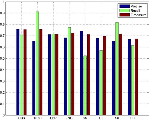
Figure 8 has shown the PR curves of different methods on Shi's dataset. Obviously, both PR curves of the HiFST method and our method are higher than the others. Furthermore, Figure 9 has shown the F-measure, precision and recall values of different methods on Shi' dataset. Although the HiFST method achieved the highest recall value, but its precision value was lower. Our method has got the highest precision values while remaining the high recall values, and then the F-measures value of our method was also the highest.

Figure 8. PR curves of different methods on Shi's dataset (Shi et al., 2014).

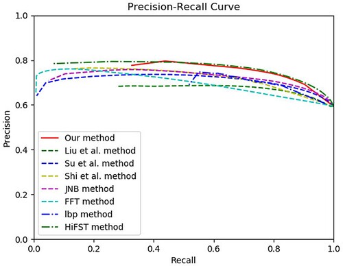
Figure 9. F-measures, precision, and recall of different methods on Shi's dataset(Shi et al., 2014).

Overall, based on these quantitative evaluations on Shi's dataset (Shi et al., 2014), our novel blur detection method has achieved higher precision and recall rate, bigger Max F-measure and S-measure scores, and less mean absolute errors, compared with other methods.

4.3.2. Subjective comparisons

For further understanding our superiority, the subjective comparisons on Shi's dataset are shown in Figures 10 and 11.

Figure 10. Examples of clear objects and blurred backgrounds in the blur detection task. Results are got by different methods on Shi's dataset. (a) Img. (b) GT. (c) FFT. (d) Su. (e) Liu. (f) Shi. (g) JNB. (h) LBP. (i) HiFST and (j) Ours.

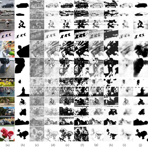
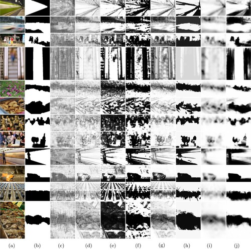
Figure 11. Examples of blurred regions in the blur detection task. Results are got by different methods on Shi's dataset. (a) Img. (b) GT. (c) FFT. (d) Su. (e) Liu. (f) Shi. (g) JNB. (h) LBP. (i) HiFST and (j) Ours.

In Figure 10, the blurness of images is caused by out of focus or by motion. All these images have something in common, that is, all of them have the clear objects and the blurred background. For this kind of image, the blur detection task is much easier. Some traditional methods, such as  Su et al. (2011) and Liu et al. (2008), JNB (Shi et al., 2015), etc., could generate the good results by using hand-crafted features. But as shown, their common disadvantage is that the backgrounds in the results are messy, and the detected objects are not complete. In contrast, the clear objects detected by our method are more complete and the blurred backgrounds are more cleaner.

In Figure 11, all original images have the blurred regions. Because the blurred parts are regions, that means no specific shapes or structures, the performance of the traditional methods decline a lot, especially in the 3rd, 6th, 7th and 8th examples. In these special cases, our method still performs well. Our method could locate the position of the blurred regions and highlight them all. Benefiting from our newly added boundary-aware loss function, our results have clearer boundaries and much closer to the ground truths.

4.3.3. Running time comparison

The comparisons of the running time of different methods, which were published during the last four years and had higher performances are shown in Table 4. We can see that the proposed method keeps a good balance between the fast running speed and high detection accuracy.

Table 4. Average running time per image in seconds on the Shi's dataset.

Methods	Shi	JNB	LBP	HiFST	Ours
Code Types	Matlab	Matlab	Matlab	Matlab	Python
Time(s)	3.14	4.51	25.4	99.5	0.20

5. Conclusions

In this paper, we present a novel boundary-aware multi-scale deep network for the blur detection. Multi-scale features extraction is benefited from the VGG-16 network. Instead of the skip connection using Conv(1*1), the contrast layers are used in this paper to enlarge the margin between the blurred areas and clear areas. For getting the same resolution with the input image, the step by step deconvolutional layers are introduced. Finally, the boundary-aware loss function is introduced to refine the results. Our method has achieved the fast evaluating speed and superior performance to the other methods, which has been demonstrated by the experiments on the public large dataset.

Disclosure statement

No potential conflict of interest was reported by the authors.

Additional information

Funding

This work is supported by the National Natural Science Funds of China [grant number 61772343], [grant number 61872429], [grant number 62072312].

Notes

1 http://www.cse.cuhk.edu.hk/leojia/projects/dblurdetect/dataset.html.

References

- Abadi, M., Agarwal, A., Barham, P., Brevdo, E., Chen, Z., Citro, C., Corrado, G. S., Davis, A., Dean, J., Devin, M., & Ghemawat, S. (2016). Tensorflow: Large-scale machine learning on heterogeneous distributed systems. arXiv preprint arXiv:1603.04467.
- Achanta, R., Hemami, S., Estrada, F., & Susstrunk, S. (2009). Frequency-tuned salient region detection. In Proceedings of the IEEE International Conference on Computer Vision and Pattern Recognition (pp. 1597–1604). https://doi.org/10.1109/CVPR.2009.5206596.
- Bae, S., & Durand, F. (2007). Defocus magnification. Computer Graphics Forum, 26(3), 571–579. https://doi.org/10.1111/cgf.2007.26.issue-3
- Chakrabarti, A., Zickler, T., & Freeman, W. T. (2010). Analyzing spatially-varying blur. In Proceedings of the IEEE International Conference on Computer Vision and Pattern Recognition (pp. 2512–2519). https://doi.org/10.1109/CVPR.2010.5539954.
- Chen, Y. H., Chang, C. C., & Hsu, C. Y. (2020). Content-based image retrieval using block truncation coding based on edge quantization. Connection Science, 32(4), 431–448. https://doi.org/10.1080/09540091.2020.1753174
- Dong, C., Loy, C. C., He, K., & Tang, X. (2015). Image super-resolution using deep convolutional networks. IEEE Transactions on Pattern Analysis and Machine Intelligence, 38(2), 295–307. https://doi.org/10.1109/TPAMI.2015.2439281
- Elder, J. H., & Zucker, S. W. (1998). Local scale control for edge detection and blur estimation. IEEE Transactions on Pattern Analysis and Machine Intelligence, 20(7), 699–716. https://doi.org/10.1109/34.689301
- Golestaneh, S. A., & Karam, L. J. (2017). Spatially-varying blur detection based on multiscale fused and sorted transform coefficients of gradient magnitudes. In Proceedings of the IEEE Conference on Computer Vision and Pattern Recognition (pp. 596–605). https://doi.org/10.1109/CVPR.2017.71.
- Honari, S., Yosinski, J., Vincent, P., & Pal, C. (2016). Recombinator networks: Learning coarse-to-fine feature aggregation. In Proceedings of the IEEE International Conference on Computer Vision and Pattern Recognition (pp. 5743–5752). https://doi.org/10.1109/CVPR.2016.619.
- Jiang, P., Ling, H., Yu, J., & Peng, J. (2013). Salient region detection by ufo: Uniqueness, focusness and objectness. In Proceedings of the IEEE International Conference on Computer Vision (pp. 1976–1983). https://doi.org/10.1109/ICCV.2013.248.
- Kang, K., Ouyang, W., Li, H., & Wang, X. (2016). Object detection from video tubelets with convolutional neural networks. In Proceedings of the IEEE International Conference on Computer Vision and Pattern Recognition (pp. 817–825). https://doi.org/10.1109/CVPR.2016.95.
- Kingma, D. P., & Ba, J. (2015). Adam: A method for stochastic optimization. In International Conference on Learning Representations 2015. https://de.arxiv.org/pdf/1412.6980.
- Levin, A. (2007). Blind motion deblurring using image statistics. In Proceedings of Advances in Neural Information Processing Systems (pp. 841–848). https://dl.acm.org/doi/10.5555/2976456.2976562.
- Liu, R., Li, Z., & Jia, J. (2008). Image partial blur detection and classification. In Proceedings of the IEEE International Conference on Computer Vision and Pattern Recognition (pp. 1–8). https://doi.org/10.1109/CVPR.2008.4587465.
- Liu, H. Y., Wang, Y. P., & Fan, N. L. (2020). A hybrid deep grouping algorithm for large scale global optimization. IEEE Transactions on Evolutionary Computation, 24(6), 1112–1124. https://doi.org/10.1109/TEVC.4235
- Lu, C., Shi, J., & Jia, J. (2013). Abnormal event detection at 150 fps in Matlab. In Proceedings of the IEEE International Conference on Computer Vision (pp. 2720–2727). https://doi.org/10.1109/ICCV.2013.338.
- Lu, Y., Stafford, T., & Fox, C. (2016). Maximum saliency bias in binocular fusion. Connection Science, 28(3), 258–269. https://doi.org/10.1080/09540091.2016.1159181
- Ma, K., Fu, H., Liu, T., Wang, Z., & Tao, D. (2018). Deep blur mapping: Exploiting high-level semantics by deep neural networks. IEEE Transactions on Image Processing, 27(10), 5155–5166. https://doi.org/10.1109/TIP.83
- Milletari, F., Navab, N., & Ahmadi, S. A. (2016). V-net: Fully convolutional neural networks for volumetric medical image segmentation. In Proceedings of the IEEE International Conference on 3d Vision (pp. 565–571). https://doi.org/10.1109/3DV.2016.79.
- Newell, A., Yang, K., & Deng, J. (2016). Stacked hourglass networks for human pose estimation. In Proceedings of the European Conference on Computer Vision (pp. 483–499). https://doi.org/10.1007/978-3-319-46484-8_29.
- Park, J., Tai, Y. W., Cho, D., & So Kweon, I. (2017). A unified approach of multi-scale deep and hand-crafted features for defocus estimation. In Proceedings of the IEEE International Conference on Computer Vision and Pattern Recognition (pp. 1736–1745). https://doi.org/10.1109/CVPR.2017.295.
- Pinheiro, P. O., Lin, T. Y., Collobert, R., & Dollár, P. (2016). Learning to refine object segments. In Proceedings of European Conference on Computer Vision (pp. 75–91). https://doi.org/10.1007/978-3-319-46448-0_5.
- Shi, J., Xu, L., & Jia, J. (2014). Discriminative blur detection features. In Proceedings of the IEEE International Conference on Computer Vision and Pattern Recognition (pp. 2965–2972). https://doi.org/10.1109/CVPR.2014.379.
- Shi, J., Xu, L., & Jia, J. (2015). Just noticeable defocus blur detection and estimation. In Proceedings of the IEEE International Conference on Computer Vision and Pattern Recognition (pp. 657–665). https://doi.org/10.1109/CVPR.2015.7298665.
- Simonyan, K., & Zisserman, A. (2015). Very deep convolutional networks for large-scale image recognition. In International Conference on Learning Representations 2015. https://arxiv.org/abs/1409.1556.
- Srivastava, V., & Biswas, B. (2020). CNN-based salient features in HSI image semantic target prediction. Connection Science, 32(2), 113–131. https://doi.org/10.1080/09540091.2019.1650330
- Su, B., Lu, S., & Tan, C. L. (2011). Blurred image region detection and classification. In Proceedings of the ACM International Conference on Multimedia (pp. 1397–1400). https://dl.acm.org/doi/10.5555/1785794.1785825.
- Sun, C., Wang, D., Lu, H., & Yang, M. H. (2018). Learning spatial-aware regressions for visual tracking. In Proceedings of the IEEE International Conference on Computer Vision and Pattern Recognition (pp. 8962–8970). https://doi.org/10.1109/CVPR.2018.00934.
- Sun, X., Zhang, X., Zou, W., & Xu, C. (2017). Focus prior estimation for salient object detection. In Proceedings of the IEEE International Conference on Image Processing (pp. 1532–1536). https://doi.org/10.1109/ICIP.2017.8296538.
- Taha, A. A., & Hanbury, A. (2015). Metrics for evaluating 3D medical image segmentation: analysis, selection, and tool. BMC Medical Imaging, 15(1), 29. https://doi.org/10.1186/s12880-015-0068-x
- Tai, Y. W., & Brown, M. S. (2009). Single image defocus map estimation using local contrast prior. In Proceedings of the IEEE International Conference on Image Processing (pp. 1797–1800). https://doi.org/10.1109/ICIP.2009.5414620.
- Tang, C., Hou, C., & Song, Z. (2013). Defocus map estimation from a single image via spectrum contrast. Optics Letters, 38(10), 1706–1708. https://doi.org/10.1364/OL.38.001706
- Tang, C., Wu, J., Hou, Y., Wang, P., & Li, W. (2016). A spectral and spatial approach of coarse-to-fine blurred image region detection. IEEE Signal Processing Letters, 23(11), 1652–1656. https://doi.org/10.1109/LSP.2016.2611608
- Vu, C. T., Phan, T. D., & Chandler, D. M. (2011). A spectral and spatial measure of local perceived sharpness in natural images. IEEE Transactions on Image Processing, 21(3), 934–945. https://doi.org/10.1109/TIP.2011.2169974
- Wang, Y. W., Liu, H., Wei, F., Zong, T., & Li, X. (2016). Cooperativeco-evolution with formula-based variable grouping for large-scale global optimization. Evolutionary Computation, 26(4), 569–596. https://doi.org/10.1162/evco_a_00214
- Wei, Y., Xia, W., Lin, M., Huang, J., Ni, B., Dong, J., Zhao, Y., & Yan, S. (2015). HCP: A flexible CNN framework for multi-label image classification. IEEE Transactions on Pattern Analysis and Machine Intelligence, 38(9), 1901–1907. https://doi.org/10.1109/TPAMI.2015.2491929
- Wu, Z., Gao, Y., Li, L., Xue, J., & Li, Y. (2019). Semantic segmentation of high-resolution remote sensing images using fully convolutional network with adaptive threshold. Connection Science, 31(2), 169–184. https://doi.org/10.1080/09540091.2018.1510902
- Xu, Z., & Zhang, W. (2020). Hand segmentation pipeline from depth map: an integrated approach of histogram threshold selection and shallow CNN classification. Connection Science, 32(2), 162–173. https://doi.org/10.1080/09540091.2019.1670621
- Xue, X., & Wang, Y. (2015). Optimizing ontology alignments through a memetic algorithm using both match fmeasure and unanimous improvement ratio. Artificial Intelligence, 223, 65–81. https://doi.org/10.1016/j.artint.2015.03.001
- Xue, X., & Wang, Y. (2016). Using memetic algorithm for instance coreference resolution. IEEE Transactions on Knowledge and Data Engineering, 28(2), 580–591. https://doi.org/10.1109/TKDE.2015.2475755
- Yan, Q., Xu, L., Shi, J., & Jia, J. (2013). Hierarchical saliency detection. In Proceedings of the IEEE International Conference on Computer Vision and Pattern Recognition (pp. 1155–1162). https://doi.org/10.1109/CVPR.2013.153.
- Ye, M., Wang, Y., Dai, C., & Wang, X. (2016). A hybrid genetic algorithm for minimum exposure path problem of wireless sensor network based on a numerical functional extreme model. IEEE Transactions on Vehicular Technology, 65(10), 8644–8657. https://doi.org/10.1109/TVT.2015.2508504
- Yi, X., & Eramian, M. (2016). LBP-based segmentation of defocus blur. IEEE Transactions on Image Processing, 25(4), 1626–1638. https://doi.org/10.1109/TIP.2016.2528042
- Zhang, X., Wang, R., Jiang, X., Wang, W., & Gao, W. (2016). Spatially variant defocus blur map estimation and deblurring from a single image. Journal of Visual Communication and Image Representation, 35, 257–264. https://doi.org/10.1016/j.jvcir.2016.01.002
- Zhang, P., Wang, D., Lu, H., Wang, H., & Yin, B. (2017). Learning uncertain convolutional features for accurate saliency detection. In Proceedings of the IEEE International Conference on Computer Vision (pp. 212–221). https://doi.org/10.1109/ICCV.2017.32.
- Zhang, K., Zuo, W., Chen, Y., Meng, D., & Zhang, L. (2017). Beyond a gaussian denoiser: Residual learning of deep cnn for image denoising. IEEE Transactions on Image Processing, 26(7), 3142–3155. https://doi.org/10.1109/TIP.83
- Zhao, J., Feng, H., Xu, Z., Li, Q., & Tao, X. (2013). Automatic blur region segmentation approach using image matting. Signal, Image and Video Processing, 7(6), 1173–1181. https://doi.org/10.1007/s11760-012-0381-6
- Zhu, X., Zuo, J., & Ren, H. (2020). A modified deep neural network enables identification of foliage under complex background. Connection Science, 32(1), 1–15. https://doi.org/10.1080/09540091.2019.1609420
- Zhuo, S., & Sim, T. (2011). Defocus map estimation from a single image. Pattern Recognition, 44(9), 1852–1858. https://doi.org/10.1016/j.patcog.2011.03.009
- Zou, K. H., Warfield, S. K., Bharatha, A., Tempany, C. M., Kaus, M. R., Haker, S. J., Wells III, W. M., Jolesz, F. A., & Kikinis, R. (2004). Statistical validation of image segmentation quality based on a spatial overlap index. Academic Radiology, 11(2), 178–189. https://doi.org/10.1016/S1076-6332(03)00671-8