Cost-sensitive regression learning on small dataset through intra-cluster product favoured feature selection

Abstract

Massive regression and forecasting tasks are generally cost-sensitive regression learning problems with asymmetric costs between over-prediction and under-prediction. However, existing classic methods, such as clustering and feature selection, are subject to difficulties in dealing with small datasets. As one of the key challenges, it is difficult to statistically validate the importance of features using traditional algorithms (e.g. the Boruta algorithm) owing to insufficient available data. By leveraging the feature information intra-cluster (item group with similar attributes), we propose an intra-cluster product favoured (ICPF) feature selection algorithm to select the information based on the traditional filtering method (specifically the Boruta algorithm in our study). The experimental results show that the ICPF algorithm significantly reduces the number of dimensions of the selected feature set and improves the performance of cost-sensitive regression learning. The misprediction cost decreased by 33.5% (linear-linear cost function) and 32.4% (quadratic-quadratic cost function) after adopting the ICPF algorithm. In addition, the advantage of the ICPF algorithm is robust to other regression models, such as random forest and XGboost.

Keywords:

• Cost-sensitive regression
• demand forecasting
• small dataset
• asymmetric cost function
• feature selection
• information filtering

1. Introduction

Cost-sensitive regression learning (CSRL) is an important branch of machine learning (ML) and plays a critical role in decision science. CSRL is pervasive in business operations and management, such as demand forecasting, real estate assessment, purchase rate forecasting, system reliability estimation, and bank loan charge-off forecasting (Bansal et al., 2008). For instance, the result of CSRL would assist purchasing officers in determining the optimal order quantities of different products.

In the realm of regression learning, there are two opposing errors: over-prediction and under-prediction errors. In the context of cost-insensitive regression learning (CIRL), which is the most widely studied in the forecasting domain, misprediction incurs identical costs regardless of over-prediction or under-prediction. In general, the modellers simply adopt a misprediction error to measure the empirical loss of the regression learning model. Lessmann and Voß (2017) used symmetric cost functions (e.g. the mean square error) to evaluate the prediction accuracy.

However, concerning CSRL, there is cost asymmetry with different costs owing to over-predictions and under-predictions. For example, in forecasting the demand for “dresses” an over-prediction may incur an inventory holding cost, whereas an under-prediction would generate a loss of orders with a difference in cost from the inventory holding cost. To solve these problems, we should train the model based on a cost minimisation rather than the error criterion, which is what the term “cost-sensitive” refers to. Crone (2010) proposed the asymmetric cost of error functions, the experimental results of which illustrate that they have a significant potential to improve the quality of decision-making.

A large amount of data is typically required to train ML models and approach the true mapping between the features and target value by as much as possible, including neural networks (Crone, 2002; Dai & Wang, 2021; Phani Narasimham & Sai Pragathi, 2019; Onan & Korukoğlu, 2017; Wang et al., 2021; Zhao et al., 2020) and support vector machines (Kim, 2003; Mohammadi & Amiri, 2019). For tree-based algorithms, such as random forest (Boehmke & Greenwell, 2019) and XGboost (Zhou et al., 2019), which require a relatively smaller sample size for model training than other ML models, more data are needed to train the model and learn the parameters than traditional statistical models (e.g. time series). In addition, in the era of big data, a higher dimension of information is available, such that we can extract a large number of features from the information hidden in the original data. This requires more samples for feature selection in the process of feature engineering and model training.

However, a small dataset, which is insufficient for ML model training, is ubiquitous in practice. For instance, newly launched products have only a short sales history. Similarly, in the inventory decision of seasonal products (e.g. fruits) that are frequently updated, many merely have few historical sales records. Moreover, as e-commerce and new retailing flourish, the frequency of product updating has accelerated. There is an increasing number of short life-cycle products in the market with little historical data. Thus, it is inevitable for us to conduct CSRL tasks with small datasets (Chang et al., 2015; Li & Liu, 2009).

CSRL may exhibit a weak performance on a small dataset. First, there may be a large number of irrelevant, redundant, and highly noisy features remaining after the feature selection processing. With an insufficient number of samples to identify the important features, it is difficult to statistically validate the significance of important measures and filter information in the selection algorithm. Second, the small dataset incurs a higher bias of the trained model. Fewer samples imply a lower probability of the model going through all possible patterns and a smaller number of patterns available for the model.

Traditionally, many solutions have been proposed to deal with machine learning on small datasets, such as an increase in the sample size (e.g. virtual data and clustering) (Huang & Moraga, 2004; Li et al., 2010; Zhou & Liu, 2006) and dimensionality reduction (feature selection or PCA) (Chandrashekar & Sahin, 2014; Too & Abdullah, 2020). Nonetheless, because they are developed in a cost-insensitive context and take no account of the asymmetry cost, these solutions tend to have a low efficiency. For instance, in the context of CSRL, similar products are classified into a single cluster. The ML model was trained by feeding the training data of the products in the cluster. Assuming that the over-prediction cost of product A in the cluster may be higher than the under-prediction cost, the opposite is true for product B. To minimise the loss in the training process, the training dataset from product A manipulates the model to under-prediction (decreasing the service level to avoid inventory cost). However, the input from product B tends to modulate the model to over-prediction (increasing the service level in the case of stockouts). As a result, the training of the model faces the dilemma of minimising the loss of data from product A at the expense of B or minimising the loss of data from B sacrificing A. Hence, traditional machine learning methods that deal with small datasets have deficiencies in cost-sensitive regression learning. Therefore, it is imperative to develop new solutions to address cost-sensitive regression learning.

We focus on reducing the number of dimensions of the feature set to improve the performance of cost-sensitive regression learning on a small dataset by increasing the matching level of the feature dimension and sample size. A new dimensionality reduction (feature selection) method, called the intra-cluster product favoured (ICPF) algorithm, is proposed, which integrates clustering and classic dimensionality reduction methods. First, we cluster the items (products) according to their attributes. Second, we use the traditional feature selection algorithm (the Boruta algorithm in our study) to select important features. Third, for each selected feature of each item, the frequency of importance is counted and sorted in descending order. Finally, we further select the features with the top frequency to train the model, where the number is related to the length of the data.

We estimate the performance of the proposed algorithm ICPF in the cost-sensitive regression learning task of demand forecasting to optimise the inventory cost using desensitised data from mainstream e-commerce in China. Cost-sensitive regression learning using the Boruta algorithm to select the features is chosen as a benchmark case. The ICPF algorithm is adopted after the feature selection of the Boruta algorithm. We employ a backpropagation neural network as the regression learning model, considering two classic types of loss function: linear-linear cost (LLC) and quadratic-quadratic cost (QQC).

The experimental results show that the ICPF significantly improves the performance of regression learning. First, the average number of selected feature sets across the 189 items decreased from 15 (Boruta algorithm) to 6 (Boruta + ICPF). Second, the average misprediction cost is reduced by 33.5% (LLC) and 32.4% (QQC), in contrast to the benchmark. Finally, the advantage of the ICPF algorithm is robust to other ML models, such as random forest and XGboost. The contributions of our study are twofold.

1. An efficient and robust novel algorithm, called ICPF, is used to filter information (features). This algorithm is easily applicable with a low complexity and fast implementation and does not require significant computational resources. The performance of the ICPF algorithm is robust to the primary feature selection methods and machine learning models.

2. An improved system for cost-sensitive regression learning on a small dataset for decision-making purposes is applied. Based on the traditional system, including the feature selection algorithm and the neural network model, we integrate the ICPF algorithm into the system to better address the tasks of CSRL on a small dataset.

The remainder of this paper is organised as follows: Section 2 summarises the relevant studies. Section 3 briefly introduces the research problems and objectives of this paper. Section 4 proposes the ICPF algorithm in detail. Section 5 describes the results of the experiment conducted to estimate the effectiveness of the ICPF algorithm. Finally, section 6 provides some concluding remarks regarding this paper.

2. Literature review

In this section, we review the relevant studies on cost-sensitive regression learning problems and predictions in the context of small datasets, as shown in Table 1.

Table 1. Related studies.

Topics	Perspective	Related studies
Cost-sensitive learning	Ex-ante rescaling	Zhou and Liu (2006), Tsou and Lin (2019), Cui et al. (2014), Liu et al. (2011), Wen et al. (2021).
	Model manipulation	Crone et al. (2005), Crone (2002), Ye and Luo (2020), Nunzio (2014).
	Ex-post modification	Bansal et al. (2008), Zhao et al. (2011), Zhang and Garcia (2015).
Learning on small dataset	Increasement of sample size	Niyogi et al. (1998), Li et al. (2003), Li and Wen (2014), Chang et al. (2014).
	Dimensionality reduction	Baumgartner et al. (2004), Kursa and Rudnicki (2010), Chandrashekar and Sahin (2014), Micallef et al. (2017), Mishra and Singh (2020).
	Learning methods	Huang and Moraga (2004), Chen et al. (2005), Mao et al. (2006), Li and Liu (2009), Li, Chang, et al. (2012), Guo et al. (2017), Luo and Paal (2021).

2.1. Cost-sensitive learning

In the realm of cost-sensitive regression learning, the key challenge is cost asymmetry. To address this problem, three different procedures are introduced: “Ex-ante Rescaling” of the samples before learning, “Model Manipulation” of the learning models during the process of learning, and “Ex-post Modification” after learning.

Ex-ante Rescaling. This procedure has been widely applied to classification problems with imbalanced samples, including a re-sampling of the samples (Liu et al., 2011; Tsou & Lin, 2019) and a re-weighting method (Zhou & Liu, 2006). Re-sampling is a type of biased sampling, which includes under-sampling and over-sampling. The category ratio of the training set samples is changed by adjusting the number of samples in different categories to balance the impact of cost differences on the learning model. Re-weighting involves weighting different classes of samples according to cost. The weight is reweighted according to the corresponding cost level. Moreover, by integrating self-paced learning and spectral rotation clustering in a unified learning framework, Wen et al. (2021) presented one-step spectral rotation clustering for imbalanced high-dimensional data to address the imbalance problem of classification. However, the ex-ante rescaling of samples, which is prone to cause an information distortion, has rarely been applied in regression learning.

Model manipulation. The loss function of the trained model is manipulated according to the over-prediction and under-prediction costs. Previous studies have mainly focussed on neural networks, tree methods, and support vector machines. Crone et al. (2005) used a multi-hidden neural network to construct a cost-sensitive loss function to conduct regression learning and forecast product sales. However, its loss function only considers an absolute error. Crone (2002) proposed a set of asymmetric cost functions as a new loss function to train a neural network for regression learning. Di Nunzio (2014) introduced a new decision function for cost-sensitive Naïve Bayes classifiers. Iranmehr et al. (2019) introduced a constructive procedure to extend the standard loss function of Support Vector Machine to optimise the classifier with respect to class imbalance or class costs.

These studies considered cost asymmetry when training the regression model. Nonetheless, none of them have a negative effect on the performance of the models caused by insufficient samples in the dataset. Our study considers two loss functions: linear (absolute) and quadratic (square) errors. A new algorithm is proposed to improve regression learning with asymmetric costs in the context of small datasets.

Ex-post Modification. This method works by adding an adjustment function after training the benchmark learner without cost asymmetry. Bansal et al. (2008) recently proposed a “re-adjustment” algorithm for cost-sensitive classification learning. Zhao et al. (2011) proposed an extended cost-sensitive regression adjustment method to minimise the average error prediction under an asymmetric cost structure. Zhang and García (2015) developed a new classifier by adding an adaptation function to the base classifier and updating the adaptation function parameter according to the streaming data samples. As an advantage, it does not need to retrain the learning model and improve the agility of the prediction model. However, this framework is generally criticised because it cannot guarantee the Bayesian continuity of the loss function and the effectiveness of the readjustment (Zhao et al., 2011). Thus, we focus on the model manipulation framework.

2.2. Learning on small dataset

The prediction of small datasets is universal in various industries such as manufacturing and the financial and retail industries (Bansal et al., 2008; Chang et al., 2019). The small size of the sample will cause challenges in the forecasting for small datasets, such as how to extract more effective information from such dataset (Li & Liu, 2012). Incomplete data may cause the trained model to not fully represent the real data structure, or cause model training to appear overfitting (Li & Liu, 2012; Li, Liu, et al., 2012). Some effective machine learning models tend to be unstable on small datasets (Li & Wen, 2014).

In the existing research, there are three main frameworks to be applied in regression and forecasting of small datasets:

Increase in sample size. This is the simplest solution to address the problem with small datasets. For instance, Niyogi et al. (1998) proposed an algorithm that uses prior knowledge obtained from a given small training set to generate virtual samples. Li et al. (2003) introduced a functional virtual population (FVP) to generate more virtual samples. Li and Wen (2014) constructed virtual samples using genetic algorithm-based virtual sample generation to improve the learning robustness on a small dataset.

Some others consider resorting to clustering algorithms. Li et al. (2003) adopted a new clustering algorithm to solve the problem of small sample size predictions. Moreover, they integrated data clustering and virtual sample generation methods by identifying the data structure and extending it to higher dimensions to improve the predictive capability of the trained model (Li et al., 2010).

However, these methods may not necessarily work in scenarios with asymmetric costs, which will undermine the effectiveness as the sample size increases. There are different cost levels for under-prediction and over-prediction. The learning capability of the ML model may be counteracted by these two scenarios, that is, a good fitness on the samples with an under-prediction error would generate poor fitness on those with an over-prediction. Simply increasing the sample size will not solve this problem.

Dimensionality reduction. Reducing the number of features, usually resorting to feature selection, is an effective solution to address the problem of learning on a small dataset. Chandrashekar and Sahin (2014) introduced an overview of feature selection methods that can be applied to a wide array of machine learning problems. These methods are grouped into three classes: filter, wrapper, and embedded. By extending the information system with “shadow attributes” that are random by design, a random forest model is able to decide which attributes are indeed important (with a statistically valid significance of the feature importance). Micallef et al. (2017) presented a novel approach using an interactive elicitation of knowledge on the feature relevance to guide the selection of features and thus improve the prediction accuracy for small datasets. Another group of studies classifies features into clusters and replaces the feature set with the corresponding feature centroid of the cluster (Baumgartner et al., 2004; Onan, 2017).

Some others combine feature selection with ensemble learning methods (Liu et al., 2019; Onan, 2018a; Onan & Korukoğlu, 2016; Onan & Tocoglu, 2020; Onan et al., 2016). Onan and Korukoğlu (2017) proposed an integrated approach to feature selection that combines several separate lists of features derived from different feature selection methods to produce a more robust and efficient subset of features. Later, he proposed a psycholinguistic approach to twitter sentiment analysis to select appropriate feature subsets in sentiment analysis and integrate them (Onan, 2018b). However, this method was not considered in our study because of its high complexity, large computational amount and its failure to improve feature screening ability.

Our study is similar to that of Mishra and Singh (2020). They introduced a wrapper feature selection method called FS-MLC, which uses clustering to find the similarity among features and example-based precision, and to rank the features. The number of features is reduced by selecting a single representative feature to represent multiples within a cluster. However, our dimensionality reduction method differs from FS-MLC in terms of the usage of clusters. In our study, we group the items rather than features into clusters and resort to the feature importance information of intra-clustered items to select the features.

Learning Methods. A number of machine learning methods have been developed for classification on small datasets, including a regularised linear discriminant analysis and transfer learning method (Chen et al., 2005; Li et al., 2018). Moreover, Mao et al. (2006) integrated techniques for creating new learning samples and support vector machine to obtain posterior probabilities with a neural network model to improve the learning accuracy of small datasets.

Other studies have focussed on the realm of regression learning, including diffusion neural network, data trend estimation techniques, omega-trend-diffusion techniques, central location data tracking methods, structure-based data transformation methods, domain knowledge, and transfer learning methods (Guo et al., 2017; Huang & Moraga, 2004; Li, Chang, et al., 2012; Luo & Paal, 2021). However, few studies have paid attention to cost-sensitive regression learning on small datasets. Our paper focuses on a feature dimension reduction rather than the development of new learning models.

3. Research questions

3.1. Background

In the real world, the costs (consequences) of under-prediction and over-prediction errors are universally different, for example, demand forecasting, bank loan charge-off forecasting, estate assessment, and system reliability estimation (Bansal et al., 2008; Carbonneau et al., 2011; Lin & Chou, 2020). For instance, in the realm of demand forecasting, an over-prediction causes an overstock and brings about costs, including holding and capital costs, as well as a deterioration of the inventory. By contrast, an under-prediction leads to product shortages and incurs an out-of-stock cost. The costs of these two errors differ to each other. Thus, efforts should be made to minimise the cost generated by a prediction error (called a “misprediction cost” in this article), rather than simply error metrics such as the average squared error.

The regression learning between cost-sensitive (asymmetric cost) and cost-insensitive (symmetric cost) differs according to the setting of the cost function (performance measure). For example, the objective of the regression problem in forecasting the demand of product i is to minimise the inventory cost with a sample set ${\mathbf{S}}_i=\{⟨{\mathbf{x}}_j^i,y_j^i⟩,j=1,2,\dots ,n_i\}$. The learned regression model refers to a mapping from ${\mathbf{x}}_j^i$ to $y_j^i$, that is, $f:{\mathbf{x}}_j^i\to y_j^i$, where $y_j^i$ is the demand (dependent variable) and ${\mathbf{x}}_j^i$ indicates the feature (independent variable) vector of sample j. Assuming that the prediction error $e_j$ of the jth sample produces a misprediction cost $C(e_j)$, the average misprediction cost (Zhao et al., 2011) of the mapping f can be defined as follows: (1) $\begin{array}{rl}A{C}^i& =\frac{1}{n_i}\sum _{j=1}^{n_i}C(e_j)\\ & =\frac{1}{n_i}\sum _{j=1}^{n_i}C(f({\mathbf{x}}_j^i)-y_j^i).\end{array}$(1) In the context of a symmetric misprediction cost, regular regression models (e.g. linear regression and neural network models) assume a symmetric cost. Symmetric cost refers to $C(e_j)=C(-e_j)$ for a misprediction error. Consequently, the cost of a misprediction becomes constant in (1(1) $\begin{array}{rl}A{C}^i& =\frac{1}{n_i}\sum _{j=1}^{n_i}C(e_j)\\ & =\frac{1}{n_i}\sum _{j=1}^{n_i}C(f({\mathbf{x}}_j^i)-y_j^i).\end{array}$(1) ). The cost function $A{C}^i$, which is essentially the prediction error function, is usually rewritten as (2) $A{C}^i=\frac{1}{n_i}\sum _{j=1}^{n_i}|f({\mathbf{x}}_j^i)-y_j^i|.$(2) In the context of an asymmetric misprediction cost, for product i, we use $c_o^i$ and $c_u^i$ to denote the cost of an over-prediction and under-prediction, respectively. The misprediction cost with the prediction of the jth sample ${\hat{y}}_j^i=f({\mathbf{x}}_j^i)$ (where the true value equals $y_j^i$) can be defined as follows: (3) $c_r^i=\{\begin{array}{ll}{c}_o^i,& {\hat{y}}_j^i\ge y_j^i;\\ c_u^i,& {\hat{y}}_j^i<y_j^i.\end{array}$(3) The cost minimisation problem of regression learning is transformed into a cost function, i.e. Equation (4(4) $\begin{array}{rl}A{C}^i& =\frac{1}{n_i}\sum _{j=1}^{n_i}{c}_r^i\left|\begin{array}{c}{\hat{y}}_j^i-y_j^i\end{array}\right|\\ & =\frac{1}{n_i}\sum _{j=1}^{n_i}[c_o^i{({\hat{y}}_j^i-y_j^i)}^{+}+c_u^i{({\hat{y}}_j^i-y_j^i)}^{-}].\end{array}$(4) ), which is a typical newsvendor problem in the field of inventory management: (4) $\begin{array}{rl}A{C}^i& =\frac{1}{n_i}\sum _{j=1}^{n_i}{c}_r^i\left|\begin{array}{c}{\hat{y}}_j^i-y_j^i\end{array}\right|\\ & =\frac{1}{n_i}\sum _{j=1}^{n_i}[c_o^i{({\hat{y}}_j^i-y_j^i)}^{+}+c_u^i{({\hat{y}}_j^i-y_j^i)}^{-}].\end{array}$(4) The ML method has been widely adopted in the areas of regression learning and forecasting. According to computational learning theory (Anthony & Biggs, 1997), a large amount of data is required to train the ML model to estimate the parameters properly and obtain a learning model with an outstanding performance. However, there are many tasks subject to small datasets, for example, the demand forecasting of new products or products having a short historical record. Data scarcity not only incurs an insufficient capability of machine learning models, but also implies a relatively high-dimensional feature set against the number of samples, which may lead to a poor feature selection and even an over-fitting of the trained ML model. The three classic feature selection frameworks, filtering, wrapping, and embedded, all suffer from insufficient screening capabilities in the context of a small dataset (Li & Liu, 2012; Niyogi et al., 1998; Verma & Salour, 2020).

To address this problem, several methods have been proposed to improve the performance of the ML model with a small dataset in the context of symmetric cost. One of the most popular solutions is clustering, which increases the number of samples in the training data to improve the feature selection and reduce the overfitting. However, it is challenging to tackle regression learning on small datasets with an asymmetric cost. Cost asymmetry renders inapplicable classic solutions (e.g. clustering) that are feasible in a task with cost symmetry.

3.2. Research objectives

In the realm of cost-sensitive regression learning (CSRL) on small datasets, the traditional solutions are inapplicable (clustering) or perform poorly (feature selection). Our study aims to propose a new solution to improve the performance of CSRL on a small dataset, which is critical in machine learning favouring decision making.

Being unable to increase the number of training data, we have to feed the small dataset (e.g. data of A or B) into the ML model. The three methods described in Section 2.2 cannot be directly applied to the context of cost-sensitive regression. Therefore, it would be reasonable to increase the matching between the dimension of the feature set and training data by designing a more effective feature selection method to reduce the number of dimensions of the information imported into the model. We attempt to improve the performance of CSRL on a small dataset at the expense of some important features (but with a small marginal contribution to the model). In the next section, we propose the ICPF feature selection algorithm to filter features (information) on a small dataset.

4. Method

The proposed algorithm integrates the traditional feature selection and clustering. In our study, we used the Boruta algorithm, which is a pervasive solution for selecting valid features and marking their importance (Kursa & Rudnicki, 2010; Liu & Setiono, 1997).

Using the Boruta algorithm, each original feature is marked as “important”, “pending”, or “unimportant”. The importance matrix Γ(boruta) for the original feature set is constructed. Here, ${\mathrm{\Gamma }}_j^i=1$ implies that feature j is important for the regression learning of item i, whereas ${\mathrm{\Gamma }}_j^i=0$ represents the opposite.¹ However, the Boruta algorithm performs poorly in the context of a small dataset. However, too many features are selected for the sample size, calling for a further selection of features (information).

The clustering algorithm can classify similar products into a single group. Although aggregating the dataset of similar items inside a cluster is infeasible, it is worth considering the use of information regarding the feature importance of the intra-cluster. This rationale pertains to the belief that a similar dataset (item) should have a similar important feature set for the regression learning model. Thus, we propose a novel algorithm based on item clustering and the Boruta algorithm to improve the feature selection for the model.

There are five critical steps used in the ICPF algorithm procedure (see Algorithm 1):

1. Employing the Boruta algorithm, every original feature is marked as “important”, “pending”, or “unimportant”,

2. Classifying the items (products) using the hierarchical clustering algorithm based on the product attributes,

3. Counting frequency of “important” marks for each original feature inside the cluster,

4. The importance frequencies of the original features are sorted,

5. Selecting $\ln m_{i,train}$ features with the top frequency for training the model, where $m_{i,train}$ is the number of training samples.

The procedure of cost-sensitive regression learning with the ICPF algorithm includes two critical processes: feature selection and model training (as shown in Figure 1). In the first step (feature selection), the ICPF algorithm is used for the secondary selection of features based on the Boruta algorithm, which operates as the primary selection.

Figure 1. Flow diagram of cost-sensitive regression learning with ICPF Algorithm 1.

Figure 1 shows the flow frame diagram of cost-sensitive regression learning with ICPF algorithm 1. Regression learning mainly includes six steps, and ICPFFS algorithm operates in the third step, namely feature selection.

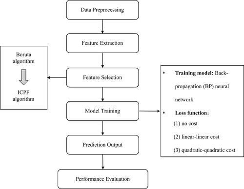
In the context of cost-sensitive regression, there are usually three commonly used frameworks according to the stage for dealing with asymmetric cost: “ex-training” (Tsou & Lin, 2019), “inter-training” (Iranmehr et al., 2019), and “post-training” (Zhou & Liu, 2006). As stated in Section 3, our study focuses on the inter-training framework because the model is able to manipulate the loss function of the learning model, e.g. directly taking the cost function as the loss function. In particular, neural networks (NNs) have the advantages of a strong learning ability and flexible loss function settings. Hence, in the second step (model training), we employ a multilayer backpropagation neural network (NN) as the regression model. Three types of loss functions are considered: no cost function (NC), linear-linear cost function (LLC), and quadratic-quadratic cost (QQC) function.

5. Datasets and experiments

5.1. Data

To verify the effectiveness of the proposed ICPF algorithm, we use desensitised time-series data from a mainstream e-commerce platform in China. The platform aims to decrease the inventory costs. The dataset contains hundreds of items with nationwide aggregated records from October 10, 2014 and December 27, 2015. We selected 189 items with a sample size (the length of the time-series data) ranging from 51 to 444.² The database consists of 30 variables, including four classes of information, i.e. item information (item ID, category, and brand), behavioural information of consumers (e.g. number of daily impressions, number of daily visitors, and frequency of “collection”), sales records (e.g. number of orders placed, number of items ordered, number of paid orders, and amount of payment), and cost information (excess and shortage of inventory, referring to over-prediction and under-prediction, respectively). With respect to the machine learning model, particularly the neural network, the sample size of the data (from one single item), with tens or hundreds of records, is relatively small. We select 189 datasets (items) with such short record length.

Table 2 provides a statistical description of the selected databases. The “sales cycle” refers to the record length of each item (time-series) in the original data, which is essentially the sample size. “Days with sales” represents the number of days of an item with sales of larger than zero. “Daily sales” indicates the daily sales per item. By averaging the daily sales of an item, “item-level daily sales” are calculated to depict the sales level of each item. By assuming that there is a sufficient inventory to fulfill demand,³ we use sales as a demand representation. For 109 items, the over-prediction cost is higher than the under-prediction cost, whereas the other items show the opposite trend. The distribution of ($c_o^i/c_u^i$) indicates that there is dramatic cost asymmetry in the dataset of each item. The statistics imply that it would be much more challenging to forecast demand (regression learning) with not only a short historical record but also cost asymmetry.

Table 2. Description of the dataset.

Statistics	Minimum	Maximum	Mean	Standard deviation
Sales cycle	51	444	268	140
Days with sales	50	444	248	130
Daily sales	0	3260	26	46
Item-level Daily sales	3	206	23	27
Over-prediction cost, $c_o^i$	8.02	95.63	46.35	9.94
Under-prediction cost, $c_u^i$	10.73	47.94	37.38	33.76
$c_o^i/c_u^i$	0.22	3.94	1.30	0.90

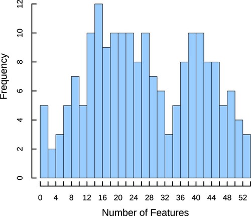
We extracted 71 features that belong to 7 classes of features from the original data, i.e. weekdays, transaction records, customer behaviours, lost sales, channel of visitors, online traffic funnel, and periodic terms. Using the Boruta algorithm, we mark the importance of features and select those with the “important” label for all items. The results demonstrate that there are still too many selected features relative to the number of samples. As shown in Figure 2, the average number of features selected from the data is 26, with a maximum of 53. The mean sample size is 206. In the ML model, the complexity of learning increases with the number of features. Thus, the number of dimensions of the feature set after the traditional filtering process is still too high compared to the sample size.

Figure 2. Histogram of the number of features selected.

This Figure describes the results of common feature selection algorithms using frequency graphs. As shown in the figure, the average number of features selected from the data is 26, the maximum number is 53, and most of the selected features are more than 15. Therefore, the dimension of the feature set processed by the traditional feature selection algorithm is still too high compared with the sample size.

5.2. Performance metrics

Equation (4(4) $\begin{array}{rl}A{C}^i& =\frac{1}{n_i}\sum _{j=1}^{n_i}{c}_r^i\left|\begin{array}{c}{\hat{y}}_j^i-y_j^i\end{array}\right|\\ & =\frac{1}{n_i}\sum _{j=1}^{n_i}[c_o^i{({\hat{y}}_j^i-y_j^i)}^{+}+c_u^i{({\hat{y}}_j^i-y_j^i)}^{-}].\end{array}$(4) ) is the objective function of the model, which implies a linear-linear cost function. However, previous studies have shown that using the quadratic cost as the loss function is more friendly to mathematical operations and exerts more punishment on large errors. Therefore, we consider both the linear-linear cost function (LLC) and quadratic-quadratic cost function (QQC) as cost-asymmetric loss functions, that is, (5) $\begin{array}{rl}LL{C}_j^i& =\{\begin{array}{ll}{c}_o^i({\hat{y}}_j^i-y_j^i),& {\hat{y}}_j^i\ge y_j^i;\\ c_u^i(y_j^i-{\hat{y}}_j^i),& {\hat{y}}_j^i<y_j^i.\end{array}\end{array}$(5) (6) $\begin{array}{rl}QQ{C}_j^i& =\{\begin{array}{ll}{c}_o^i({\hat{y}}_j^i-y_j^i{)}^2,& {\hat{y}}_j^i\ge y_j^i;\\ c_u^i(y_j^i-{\hat{y}}_j^i{)}^2,& {\hat{y}}_j^i<y_j^i.\end{array}\end{array}$(6) The average daily cost of a demand forecast on the ith product $AD{C}^i$ is calculated as follows: (7) $AD{C}^i=\{\begin{array}{ll}{\displaystyle \frac{\sum _{j=1}^{m^i}LL{C}_j^i}{m^i},}& Linear-LinearCost;\\ {\displaystyle \frac{\sum _{j=1}^{m^i}QQ{C}_j^i}{m^i},}& Quadratic-QuadraticCost.\end{array}$(7) where $m^i$ represents the sample size of the ith item.

This study uses five indicators to evaluate the effectiveness of the proposed algorithm, i.e. the average daily cost of different item training sets $AD{C}_{train}$ (in units of 100cny), average daily cost of different item test sets $AD{C}_{test}$, median of the average daily cost of the testing set $MD{C}_{test}$. The specific calculation formulas are defined as follows: (8) $\begin{array}{rl}AD{C}_{train}& =\frac{\sum _{i=1}^{n}AD{C}_{train}^i}{n}.\end{array}$(8) (9) $\begin{array}{rl}AD{C}_{test}& =\frac{\sum _{i=1}^{n}AD{C}_{test}^i}{n}.\end{array}$(9) (10) $\begin{array}{rl}MD{C}_{test}& =Median\{AD{C}_{test}^i\}.\end{array}$(10)

5.3. Experimental results

5.3.1. Results

This section introduces the experimental results of cost-sensitive regression learning using the ICPF feature selection algorithm. The codes for the experiments were programmed using Python 3.7.

As shown in Table 3, the novel feature selection method introduced in Algorithm 1 significantly reduces the number of features in the product dataset, and the number of selected features is significantly decreased by applying the ICPF algorithm; for example, the number of selected features is at most 10. On average, the mean value (the last column in Table 3) decreased from 15 to 6 after secondary selection.

Table 3. Distribution of selected feature set size.

Boruta algorithm	No. items	Boruta algorithm + ICPF	No. items
$[1,10]$	22	$[1,4]$	7
$[11,20]$	46	5	90
$[21,30]$	45	6	33
$[31,40]$	32	7	10
$[41,50]$	37	8	34
$[51,60]$	7	$[9,10]$	15
Mean	15	Mean	6

The experimental results for different measurement metrics are presented in Table 4. Here, BP_LLC_AF and BP_QQC_AF (where AF indicates all features) refer to the method using the complete original feature set with a linear-linear and quadratic-quadratic cost function, respectively. In addition, BP_LLC_Boruta and BP_QQC_Boruta denote the method using the feature set selected using the Boruta algorithm, and BP_LLC_ICPF and BP_QQC_ICPF indicate methods using the ICPF algorithm.

Table 4. Test results of different feature sets (cost unit: cny).

Method	$AD{C}_{train}$	$AD{C}_{test}$	$MD{C}_{test}$
BP_LLC_AF	468	630	280
BP_LLC_Boruta	428	540	25
BP_LLC_ICPF	314	359	179
BP_QQC_AF	488	596	278
BP_QQC_Boruta	425	512	265
BP_QQC_ICPF	330	346	184

Here, n represents the number of items. We compare the performance metrics with those from the forecasting using the Boruta algorithm for selecting the features. For a single item, the smaller the values of $AD{C}_{train}^i$ and $AD{C}_{test}^i$, the better the performance of the proposed algorithm. With respect to the entire learning task, smaller $MD{C}_{test}$ values indicate that our method is superior to the benchmark.

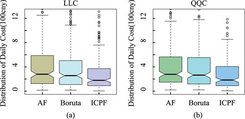
In contrast to the traditional feature selection method, the average daily prediction cost ($AD{C}_{train}$ and $AD{C}_{test}$) is significantly reduced in the model with either the LLC or QQC loss function, using the features selected by the ICPF algorithm. For instance, with the LLC loss function, the average daily misprediction cost of the test set is reduced by 33.5%, decreasing from 540 to 359. With the QQC loss function, the average misprediction cost decreased by 32.4% from 512 to 346. Moreover, as shown in Figure 3, we use a boxplot to visually compare the level of distribution of the misprediction cost. Regardless of whether the model adopts the LLC or QQC loss function, the average daily misprediction cost of the testing samples in the model using the ICPF algorithm is significantly lower than the benchmark.

Figure 3. Box-plot of average daily misprediction cost of different feature selection algorithms.

This Figure depicts the average daily misprediction cost of the three feature selection algorithms. Figure (a) shows that when the model cost loss function is LLC, the ICPF algorithm significantly reduces the average daily misprediction cost of the model. Figure (b) shows that when the cost loss function of the model is QQC, the daily misprediction cost of ICPF algorithm is also lower than that of the benchmark algorithm.

We used a single-tail paired t-test to verify the effect of the ICPF algorithm. Three pairs differing by the loss function (NC, LLC or QQC) are tested. The results in Table 5 indicate that the effect of the proposed ICPF algorithm on the misprediction cost is significant at the 0.001 level (in fact, the p-value is lower than ${10}^{-9}$). Therefore, the misprediction cost caused by the forecasting from the employment of the ICPF algorithm is significantly lower than that of the benchmark (Boruta algorithm).

Table 5. Paired sample t-test on the average daily misprediction cost.

		Average daily misprediction cost
Pairs		mean	t	df	p-value
BP_NC_Boruta	BP_NC_ICPF	211	6.69	188	$2.37\mathrm{E}-{10}^{\ast \ast \ast }$
BP_LLC_Boruta	BP_LLC_ICPF	153	6.02	188	$8.74\mathrm{E}-{09}^{\ast \ast \ast }$
BP_QQC_Boruta	BP_QQC_ICPF	135	6.14	188	$4.84\mathrm{E}-{09}^{\ast \ast \ast }$

${}^{\ast \ast \ast }p<0.001$.

All empirical results verify that the proposed ICPF algorithm, using the two steps of feature selection through item clustering, effectively reduces the number of dimensions of the feature set. As a result, the performance of the ML model in cost-sensitive regression learning is considerably improved.

5.3.2. Robust test

To inspect the reliability of the ICPF algorithm, the robustness of this algorithm is tested in this section. We consider the other two classic ML models in the field of regression learning: random forecast(“RF”) and XGboost. Table 6 presents the performance metrics of the two models using different feature selection algorithms. Feature selection includes three scenarios: all the original features are fed into the model without selection (“AF”); the feature selection using Boruta algorithm (“Boruta”); and the feature selection using ICPF algorithm (“ICPF”).

Table 6. Performance metrics of the two ML models.

ML Model	Feature selection	$AD{C}_{train}$	$AD{C}_{test}$	$MD{C}_{test}$
RF	AF	126	567	285
	Boruta	121	522	275
	ICPF	133	437	240
XG	AF	93	531	320
	Boruta	99	506	297
	ICPF	136	446	264

The results confirm that the performance improvement of the ICPF algorithm is robust under different ML models from the following two perspectives:

1. The average daily forecast cost of the test data was significantly reduced. There is a jump in cost by 22.9% (from 567 to 437) in the random forest model, whereas the cost decreases by 16.0% (from 531 to 446) in the XGboost model. Figure 4(a,b) shows boxplots of the average daily prediction cost in the testing data. Regardless of whether random forest or XGboost is used, the ICPF algorithm outperforms the benchmark in terms of both the level and concentration of the cost distribution.

2. The results of the paired t-test is consistent with statement (1). As shown in Table 7, in regression learning using random forest, the effect of the proposed ICPF algorithm on a misprediction cost is significant at the level of 0.001. Hence, the misprediction cost from the employment of the ICPF algorithm is significantly lower than that of the benchmark (Boruta algorithm). This is similar to the results of XGboost.

Figure 4. Boxplots of average daily predicted cost.

Figure 4 shows the test results of three feature selection algorithms under different algorithm models. In figure (a), the algorithm model is random forest. When ICPF is used for feature selection, the average daily misprediction cost of the test set is lower than that of the benchmark algorithm. Figure (b) shows the results of the Xgboost model. Similarly, the ICPF algorithm significantly reduces the average daily misprediction cost.

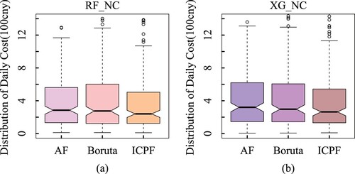
Table 7. Paired sample t-test on average daily misprediction cost.

			Average daily misprediction cost
Model	Pairs		mean	t	df	p-value
RF	Boruta	ICPF	70	4	188	$1.66\mathrm{E}-{04}^{\ast \ast \ast }$
XG	Boruta	ICPF	47	4	188	$1.39\mathrm{E}-{04}^{\ast \ast \ast }$

${}^{\ast \ast \ast }p<\mathrm{0.001.}$

Moreover, it is worth mentioning that the algorithm is robust for different primary feature selection methods. In this study, we mainly focus on the Boruta algorithm, which is classic and powerful approach used in feature engineering. However, the ICPF algorithm works independently against the primary feature selection. Adopting a distinct selection method does not change the core function of the ICPF algorithm.

In summary, the performance of the ICPF algorithm for secondary feature selection, which is proposed to tackle the challenge of cost-sensitive regression learning on a small dataset, is robust to the different loss functions (NC, LLC and QQC), a variety of ML models (Neural Network, Random Forest, and XGboost), and even the primary feature selection method carried out prior to the ICFP algorithm.

6. Conclusion

In this paper,to increase the matching between the number of dimensions of the feature set and the length of the training data, we propose the ICPF algorithm to improve the performance of the ML model by secondary select features based on the traditional feature filtering procedure. The main idea of the ICPF algorithm is utilising the selected features of other datasets (items) intra-clustered to further refine the feature set of the targeted item at the expense of less important information (features).

We evaluated the performance of the ICPF algorithm in the domain of demand forecasting with asymmetric costs using real-world online records from a mainstream platform in China. The empirical performance metrics illustrate that this could be of major help to regression learning when trying to refine a feature set. The experimental results show that the number of dimensions of the feature set is significantly reduced, with the average decreasing from 15 to 6. In the framework of a back propagation neural network, the average daily misprediction cost of the testing data decreased by 33.5% (LLC) and 32.4% (QQC). Moreover, the improvement in misprediction cost is robust on other ML models.

Our study provides several avenues for future research: (1) other loss functions are applied, such as the smooth L1; (2) this study focuses on the model manipulation without involving ex-ante rescaling or ex-post modification; (3) the proposed algorithm does not apply to a dataset with excessively small number of samples. For instance, if only 10 or 20 samples are available for a single item, cost-sensitive regression learning is infeasible, even with our method. The development of methods to handle such a small dataset would be an intriguing subject for future research.

Disclosure statement

No potential conflict of interest was reported by the author(s).

Additional information

Funding

This work was supported by the grants from National Key Research and Development Program of China under Grant (Project No. 2018YFC0831800), the National Natural Science Foundation of China (Project No. 62076092), Special Project of Foshan Science and Technology Innovation Team under Grant (Project No. FS0AA-KJ919-4402-0069), National Key R&D Program of China (Project No. 2019YFB1404901), and National Natural Science Foundation of China (Project No. 71821002).

Notes

1 In our study, those features marked as “pending” are also labelled as 0.

2 Actually, there are items with a sample size of smaller than 50. However, in the context of cost-sensitive learning, the clustering method is inapplicable. It would be more appropriate to use the time-series methods (i.e. ARIMA) for prediction if the sample size is too small. Hence, we exclude those items with a sample size of smaller than 50.

3 The assumption is reasonable because the sellers on the online platform are able to reduce the backorder by delaying the shipments.

References

- Anthony, M. H. G., & Biggs, N. (1997). Computational learning theory. Cambridge University Press.
- Bansal, G., Sinha, A. P., & Zhao, H. (2008, December). Tuning data mining methods for cost-sensitive regression: A study in loan charge-off forecasting. Journal of Management Information Systems, 25(3), 315–336. https://doi.org/10.2753/MIS0742-1222250309
- Baumgartner, R., Somorjai, R., Bowman, C., Sorrell, T., Mountford, C., & Himmelreich, U. (2004, February). Unsupervised feature dimension reduction for classification of MR spectra. Magnetic Resonance Imaging, 22(2), 251–256. https://doi.org/10.1016/j.mri.2003.08.033
- Boehmke, B., & Greenwell, B. (2019, November). Random forests. In Hands-on machine learning with R (pp. 203–219). Chapman and Hall/CRC.
- Carbonneau, R. A., Kersten, G. E., & Vahidov, R. M. (2011, January). Pairwise issue modeling for negotiation counteroffer prediction using neural networks. Decision Support Systems, 50(2), 449–459. https://doi.org/10.1016/j.dss.2010.11.002
- Chandrashekar, G., & Sahin, F. (2014, January). A survey on feature selection methods. Computers and Electrical Engineering, 40(1), 16–28. https://doi.org/10.1016/j.compeleceng.2013.11.024
- Chang, C. J., Dai, W. L., & Chen, C. C. (2015, November). A novel procedure for multimodel development using the grey silhouette coefficient for small-data-set forecasting. Journal of the Operational Research Society, 66(11), 1887–1894. https://doi.org/10.1057/jors.2015.17
- Chang, C. J., Li, D. C., Chen, C. C., & Chen, W. C. (2019, March). Extrapolation-based grey model for small-data-set forecasting. Economic Computation and Economic Cybernetics Studies and Research, 53(1), 171–182. https://doi.org/10.24818/18423264
- Chang, C. J., Li, D. C., Dai, W. L., & Chen, C. C. (2014). A latent information function to extend domain attributes to improve the accuracy of small-data-set forecasting. Neurocomputing, 129, 343–349. https://doi.org/10.1016/j.neucom.2013.09.024
- Chen, W. S., Yuen, P. C., & Huang, J. (2005, November). A new regularized linear discriminant analysis method to solve small sample size problems. International Journal of Pattern Recognition and Artificial Intelligence, 19(7), 917–935. https://doi.org/10.1142/S0218001405004344
- Crone, S. F. (2002). Training artificial neural networks for time series prediction using asymmetric cost functions. In L. Wang, J. C. Rajapakse, K. Fukushima, S.-Y. Lee, & X. Yao (Eds.), Proceedings of the 9th international conference on Neural Information Processing, ICONIP'02 (pp. 2374–2380). Springer.
- Crone, S. F. (2010). Neuronale netze zur prognose und disposition im handel. Gabler.
- Crone, S. F., Lessmann, S., & Stahlbock, R. (2005). Utility based data mining for time series analysis. In Proceedings of the 1st international workshop on utility-based data mining-UBDM'05 (pp. 59–68). Knowledge Discovery and Data Mining.
- Cui, G., Wong, M. L., & Wan, X. (2014). Cost-sensitive learning via priority sampling to improve the return on marketing and CRM investment. Journal of Management Information Systems, 29(1), 341–374. https://doi.org/10.2753/MIS0742-1222290110
- Dai, Y., & Wang, T. (2021). Prediction of customer engagement behaviour response to marketing posts based on machine learning. Connection Science, 33(4), 891–910. https://doi.org/10.1080/09540091.2021.1912710
- Di Nunzio, G. M. (2014, September). A new decision to take for cost-sensitive Naïve Bayes classifiers. Information Processing and Management, 50(5), 653–674. https://doi.org/10.1016/j.ipm.2014.04.008
- Guo, Z. G., Gao, X. G., Ren, H., Yang, Y., Di, R. H., & Chen, D. Q. (2017, December). Learning bayesian network parameters from small data sets: A further constrained qualitatively maximum a posteriori method. International Journal of Approximate Reasoning, 91, 22–35. https://doi.org/10.1016/j.ijar.2017.08.009
- Huang, C., & Moraga, C. (2004, February). A diffusion-neural-network for learning from small samples. International Journal of Approximate Reasoning, 35(2), 137–161. https://doi.org/10.1016/j.ijar.2003.06.001
- Iranmehr, A., Masnadi Shirazi, H., & Vasconcelos, N. (2019, May). Cost-sensitive support vector machines. Neurocomputing, 343, 50–64. https://doi.org/10.1016/j.neucom.2018.11.099
- Kim, K. J. (2003, September). Financial time series forecasting using support vector machines. Neurocomputing, 55(1–2), 307–319. https://doi.org/10.1016/S0925-2312(03)00372-2
- Kursa, M. B., & Rudnicki, W. R. (2010). Feature selection with the Boruta Package. Journal of Statistical Software, 36(11). https://doi.org/10.18637/jss.v036.i11
- Lessmann, S., & Voß, S. (2017, October). Car resale price forecasting: The impact of regression method, private information, and heterogeneity on forecast accuracy. International Journal of Forecasting, 33(4), 864–877. https://doi.org/10.1016/j.ijforecast.2017.04.003
- Li, D. C., Chang, C. C., & Liu, C. W. (2012, February). Using structure-based data transformation method to improve prediction accuracies for small data sets. Decision Support Systems, 52(3), 748–756. https://doi.org/10.1016/j.dss.2011.11.021
- Li, D. C., Chen, L. S., & Lin, Y. S. (2003, January). Using functional virtual population as assistance to learn scheduling knowledge in dynamic manufacturing environments. International Journal of Production Research, 41(17), 4011–4024. https://doi.org/10.1080/0020754031000149211
- Li, D. C., Chen, W. C., Liu, C. W., & Lin, Y. S. (2010, August). A non-linear quality improvement model using SVR for manufacturing TFT-LCDs. Journal of Intelligent Manufacturing, 23(3), 835–844. https://doi.org/10.1007/s10845-010-0440-1
- Li, D. C., & Liu, C. W. (2009, August). A neural network weight determination model designed uniquely for small data set learning. Expert Systems with Applications, 36(6), 9853–9858. https://doi.org/10.1016/j.eswa.2009.02.004
- Li, D. C., & Liu, C. W. (2012, March). Extending attribute information for small data set classification. IEEE Transactions on Knowledge and Data Engineering, 24(3), 452–464. https://doi.org/10.1109/TKDE.2010.254
- Li, D. C., Liu, C. W., & Chen, W. C. (2012, December). A multi-model approach to determine early manufacturing parameters for small-data-set prediction. International Journal of Production Research, 50(23), 6679–6690. https://doi.org/10.1080/00207543.2011.613867
- Li, D. C., & Wen, I. H. (2014, November). A genetic algorithm-based virtual sample generation technique to improve small data set learning. Neurocomputing, 143, 222–230. https://doi.org/10.1016/j.neucom.2014.06.004
- Li, W., Ding, S., Chen, Y., Wang, H., & Yang, S. (2018, September). Transfer learning-based default prediction model for consumer credit in China. The Journal of Supercomputing, 75(2), 862–884. https://doi.org/10.1007/s11227-018-2619-8
- Lin, Y. F., & Chou, J. (2020). Supply chain with several competing retailers and one manufacturer. International Journal on Computer Science and Engineering, 12(1), 1–6.
- Liu, H., & Setiono, R. (1997). Feature selection and classification: A probabilistic wrapper approach. Proceedings of 9th international conference on Industrial and Engineering Applications of AI and ES (pp. 419–424).
- Liu, Y., Yu, X., Huang, J. X., & An, A. (2011, July). Combining integrated sampling with SVM ensembles for learning from imbalanced datasets. Information Processing and Management, 47(4), 617–631. https://doi.org/10.1016/j.ipm.2010.11.007
- Liu, Z., Japkowicz, N., Wang, R., & Tang, D. (2019). Adaptive learning on mobile network traffic data. Connection Science, 31(2), 185–214. https://doi.org/10.1080/09540091.2018.1512557
- Luo, H., & Paal, S. G. (2021, September). Reducing the effect of sample bias for small data sets with double–weighted support vector transfer regression. Computer-Aided Civil and Infrastructure Engineering, 36(3), 248–263. https://doi.org/10.1111/mice.12617
- Mao, R., Zhu, H., Zhang, L., & Chen, A. (2006, October, 16–18). A new method to assist small data set neural network learning. 6th international conference on Intelligent Systems Design and Applications, Jian, China. IEEE. https://doi.org/10.1109/ISDA.2006.67
- Micallef, L., Sundin, I., Marttinen, P., Ammad-ud din, M., Peltola, T., Soare, M., Jacucci, G., & Kaski, S. (2017, March). Interactive elicitation of knowledge on feature relevance improves predictions in small data sets. Proceedings of the 22nd international conference on Intelligent User Interfaces (pp. 547–552).
- Mishra, N. K., & Singh, P. K. (2020, July). FS-MLC: Feature selection for multi-label classification using clustering in feature space. Information Processing and Management, 57(4), 102240–102264. https://doi.org/10.1016/j.ipm.2020.102240
- Mohammadi, F. S., & Amiri, A. (2019). TS-WRSVM: Twin structural weighted relaxed support vector machine. Connection Science, 31(3), 215–243. https://doi.org/10.1080/09540091.2019.1573418
- Niyogi, P., Girosi, F., & Poggio, T. (1998). Incorporating prior information in machine learning by creating virtual examples. Proceedings of the IEEE, 86(11), 2196–2209. https://doi.org/10.1109/5.726787
- Nunzio, G. M. D. (2014). A new decision to take for cost-sensitive Naïve Bayes classifiers. Information Processing and Management: An International Journal, 50(5), 653–674. https://doi.org/10.1016/j.ipm.2014.04.008
- Onan, A. (2017). Hybrid supervised clustering based ensemble scheme for text classification. Kybernetes the International Journal of Systems and Cybernetics, 46(2), 330–348. https://doi.org/10.1108/K-10-2016-0300
- Onan, A. (2018a). An ensemble scheme based on language function analysis and feature engineering for text genre classification. Journal of Information Science: Principles and Practice, 44(1), 28–47. https://doi.org/10.1177/0165551516677911
- Onan, A. (2018b). Sentiment analysis on twitter based on ensemble of psychological and linguistic feature sets. Balkan Journal of Electrical and Computer Engineering, 6(2), 69–77. https://doi.org/10.17694/bajece.419538
- Onan, A., Bulut, H., & Korukoğlu, S. (2016). Ensemble of keyword extraction methods and classifiers in text classification. Expert Systems with Application, 57, 232–247. https://doi.org/10.1016/j.eswa.2016.03.045
- Onan, A., & Korukoğlu, S. (2016). Exploring performance of instance selection methods in text sentiment classification. In R. Silhavy, R. Senkerik, Z. Oplatkova, P. Silhavy, & Z. Prokopova (Eds.), Artificial intelligence perspectives in intelligent systems (Vol. 464, Advances in Intelligent Systems and Computing, pp. 167–179). Springer. https://doi.org/10.1007/978-3-319-33625-1_16
- Onan, A., & Korukoğlu, S. (2017). A feature selection model based on genetic rank aggregation for text sentiment classification. Journal of Information Science, 43(1), 25–38. https://doi.org/10.1177/0165551515613226
- Onan, A., & Tocoglu, M. A. (2020). Satire identification in Turkish news articles based on ensemble of classifiers. Turkish Journal of Electrical Engineering and Computer Sciences, 28(2), 1086–1106. https://doi.org/10.3906/elk-1907-11
- Phani Narasimham, M. V. S., & Sai Pragathi, Y. V. S. (2019). Development of realistic models of oil well by modeling porosity using modified ANFIS technique. International Journal on Computer Science and Engineering, 11(7), 34–39.
- Too, J., & Abdullah, A. R. (2020). Binary atom search optimisation approaches for feature selection. Connection Science, 32(4), 406–430. https://doi.org/10.1080/09540091.2020.1741515
- Tsou, Y. L., & Lin, H. T. (2019, April). Annotation cost-sensitive active learning by tree sampling. Machine Learning, 108(5), 785–807. https://doi.org/10.1007/s10994-019-05781-7
- Verma, N. K., & Salour, A. (2020). Feature selection. Studies in Systems, Decision and Control, 256, 175–200. https://doi.org/10.1007/978-981-15-0512-6_5
- Wang, S., Zhao, H., & Nai, K. (2021). Learning a maximized shared latent factor for cross-modal hashing. Knowledge-Based Systems, 228, 107252. https://doi.org/10.1016/j.knosys.2021.107252
- Wen, G., Li, X., Zhu, Y., Chen, L., Luo, Q., & Tan, M. (2021, January). One-step spectral rotation clustering for imbalanced high-dimensional data. Information Processing and Management, 58(1), 102388–102404. https://doi.org/10.1016/j.ipm.2020.102388
- Ye, H., & Luo, Z. C. (2020). Deep ranking based cost-sensitive multi-label learning for distant supervision relation extraction. Information Processing & Management, 57(6), 102096–102110.
- Zhang, J., & García, J. (2015, April). Online classifier adaptation for cost-sensitive learning. Neural Computing and Applications, 27(3), 781–789. https://doi.org/10.1007/s00521-015-1896-x
- Zhao, H., Cao, J., Xu, M., & Lu, J. (2020, January). Variational neural decoder for abstractive text summarization. Computer Science and Information Systems, 17(2), 537–552. https://doi.org/10.2298/CSIS200131012Z
- Zhao, H., Sinha, A. P., & Bansal, G. (2011, June). An extended tuning method for cost-sensitive regression and forecasting. Decision Support Systems, 51(3), 372–383. https://doi.org/10.1016/j.dss.2011.01.003
- Zhou, Y., Li, T., Shi, J., & Qian, Z. (2019, February). A ceemdan and XGboost-based approach to forecast crude oil prices. Complexity, 2019, 4392785. https://doi.org/10.1155/2019/4392785
- Zhou, Z. H., & Liu, X. Y. (2006, January). Training cost-sensitive neural networks with methods addressing the class imbalance problem. IEEE Transactions on Knowledge and Data Engineering, 18(1), 63–77. https://doi.org/10.1109/TKDE.2006.17