COSMIC FP method in software development estimation using artificial neural networks based on orthogonal arrays

Abstract

This paper proposes a new, improved COmmon Software Measurement International Consortium function point (COSMIC FP) method that uses Artificial Neural Network (ANN) architectures based on Taguchi’s Orthogonal Array to estimate software development effort. The minimum magnitude relative error (MRE) to evaluate these architectures considering the cost effect function, the type of data used in the training, testing, and validation of the proposed models, was used. Applying the fuzzification and clustering method to obtain seven different datasets, we would like to achieve excellent reliability and accuracy of the obtained results. Besides examining the influence of four input values, we aim to reduce the risks of potential errors, increase the coverage of a wide range of different projects and increase the efficiency and success of completing many various software projects. The main contributions of our work are as follows: the influence of four input values of the COSMIC FP method on the change of mean (MRE), development of two simple ANN architectures, the attainment of a small number of performed iterations in software effort estimation (less than 7), reduced software effort estimation time, the use of different values of the International Software Benchmarking Standards Group and other datasets used in the experiment.

KEYWORDS:

• COSMIC FP
• software effort estimation
• artificial neural network design
• Taguchi Orthogonal Arrays
• robust design of the experiment
• ISBSG

1. Introduction

Existing methods of effort and cost estimation for the project development with different algorithmic techniques or applying non-algorithmic models of artificial intelligence continue to be a huge challenge and problem for the software industry and researchers in this field of software engineering (Khaw et al., 1995; Stoica & Blosiu, 1997). This leads to the fact that the assessment of effort and cost due to different conditions is still a significant activity of software project management (CHAOS Report, 2013; D. Rankovic et al., 2021). Estimates of effort below real values often lead to project cancellations or failures due to spent budgets. Additionally, this is a problem for both software companies that have already invested resources in projects and for clients who will not get the desired products or have to invest more (Goyal & Parashar, 2018; Jiang et al., 2021; Jiao et al., 2021; Qiu et al., 2021; Subasri et al., 2020). On the other hand, the estimated effort is higher than realistic conduct to uncompetitive project design bids, so software teams often fail to get and start a project. Also, it is required to enhance the existing assessment methods and mitigate these risks (Potha et al., 2021). Several methods are currently used in practice that can be applied in quantifying software in terms of size or complexity. The parameters that are taken into account are the functionalities and the influence of non-functional requirements (Di Martino et al., 2020; Ugalde et al., 2020; Younas et al., 2020). There is also a particular group of methods that directly result in the time needed to invest in the project. Analyzing the functionality or programme code makes it possible to obtain numerical values that quantify the scope of effort on a particular project. Systems that implement similar functionalities using different technologies or programming languages and/or tools may differ in the number of source lines required for implementation but will have the exact sizes expressed in functional points. As the value of a particular system is assessed based on the functionality it provides to users and not based on technology, the most important methods from this group are the Albrecht method (now known as IFPUG 4.1 method by INTER) (Cuadrado-Gallego et al., 2008), Mark II method (Mk II created by Simons) (Symons, 1988), NESMA method (created by Netherlands Software Metrics Association) (Lavazza & Liu, 2019), and COSMIC FP method (created by COmmon Software Measurement International Consortium, Full Function Point) (Quesada-López et al., 2020). The COSMIC FP method is the latest in the family of function point methods, and it is expected that other methods will change in the future to better adapt to the COSMIC FP method. It was created to overcome the problems that affected its predecessors from the mentioned family. The COSMIC FP method observes the elementary communication and data movement that is exchanged in the system. Four basic types of data movement can be exchanged between users and systems, between system components, between systems and data warehouses, and similar (Angara et al., 2018). It is possible to improve existing estimation further, using popular prediction models based on various artificial intelligence tools and the COSMIC FP method. Artificial neural networks (ANN) have proven to be a compelling idea for prediction because they can transmit information to certain elements modified by appropriate transformations and passed on to other elements (Kheyrinataj & Nazemi, 2020; Meng et al., 2017; Moosavi & Bardsiri, 2017; Sabaghian et al., 2020). The input values of the ANN represent the independent variables based on which the prediction is made. In contrast, the output values of the design effort estimate are expressed by magnitude relative error (MRE). The advantage of neural networks over linear regression with multiple variables lies in the fact that it is unnecessary to assume functional dependence as the network will detect itself in the training phase. The disadvantage lies in the fact that many experiments are needed for the network to train well. To address this shortcoming, we proposed constructing two different ANN architectures based on Taguchi’s orthogonal vector plans (a unique set of Latin Squares) (ReliaSoft Publishing, 2012; The University of York, Department of Mathematics, 2004). The ANN is associated with an Orthogonal Array (OA) with the number of parameters equalling the number of weights of the ANN. The interval containing the solution is gradually dwindling as the result of an iterative algorithm. The obtained results show that the method of Taguchi Orthogonal Arrays is an efficient philosophy for directing ANNs in learning speed, accuracy, and a smaller number of performed iterations. The contribution of this approach lies in the application of ANNs, based on Taguchi search/optimisation arrays, using COSMIC FPP as input values. Clustering and transformation of input values enable control of the heterogeneous nature of projects. The sigmoid activation function contributes to the rate of convergence. Prediction and correlation confirm the correctness, success, stability, and reliability of the proposed approach. In addition to constructing and monitoring all of these metrics, the main goal of this paper is to examine the influence of four individual input values on the change in MRE values for two different ANN architectures (ANN-L12 and ANN-L36prim) based on Taguchi Orthogonal Arrays.

This paper is structured as follows: Section 2 provides an overview of the previous studies that applied ANNs and the COSMIC FP method for software effort estimation. Section 3 describes the methodology that we will apply in our approach and experiment. Section 4 discusses the results obtained in the experimental part of the research, while the concluding remarks are given in the last section.

2. Related work

Measuring the system based on code analysis brings with it various problems. For that reason, the researchers and practicers tried to find an appropriate measure that would not have the issues of a technical nature that source code lines have. One of the measures introduced is the measure of functional points that determine the system's functionality (Popović & Bojić, 2012). Over the last decade, it is considered that COSMIC FP measurement in organisations, as the youngest method from the function point family, is the quality that is suitable for early software development estimation. Besides, COSMIC functional size is widely used as an estimation methodology for proper management. Researches in (Hussain et al., 2013; Sakhrawi et al., 2020; Salmanoglu et al., 2017) showed that despite other new measurements such as story points in agile methodologies, in all three examined cases COSMIC based estimation was more precise and effective. The study (Fehlmann & Santillo, 2010) presented the comparisons between the impact of functional enhancement size generated from COSMIC and IFPUG (Popović & Bojić, 2012) methods on the effort prediction. COSMIC functional size gave better results as input for predicting software enhancement effort. The paper (Ochodek et al., 2020) defined an approximation model with a convolutional neural network and achieved the prediction accuracy using a word-embedding model trained on Wikipedia+Gigaworld. They also described the requirements in the form of use cases. The other study (Bagriyanik & Karahoca, 2018) proposed different machine learning algorithms to identify software COSMIC Function Point measurement development. The authors in (Xia et al., 2008, 2015) proposed calibration of Function Point (FP) complexity weights and an FP calibration model called Neuro-Fuzzy Function Point Calibration Model (NFFPCM). They used the International Software Benchmarking Standards Group (ISBSG) repository and showed improved mean magnitude relative error (MMRE) accuracy in software effort estimation after calibration. They used only the parts of the ISBSG datasets, while in this paper, the whole dataset was used without any calibration or tunning. Also, we present the clustering method of input values for the entire dataset, besides fuzzification and fewer required iterations on different combinations of datasets from the ISBSG repository. Furthermore, we introduce two other validation datasets to confirm the obtained results. In (Di Martino et al., 2016), the main objective was to investigate if COSMIC FP is more effective than traditional FPA for Web effort estimation using an industrial dataset. The results showed that the new prediction model based on estimated COSMIC FP sizes was more precise. The paper (Kaur & Kaur, 2019) described the importance of evaluating effort for testing mobile applications and predict the test effort considering COSMIC FP characteristics and factors. They also used the prediction on two criteria to predict test effort, which is not suitable for the early stage estimation. In our approach, we use the prediction on three criteria to confirm the reliability of the proposed models (N. Rankovic et al., 2021). Additionally, the correlation coefficients (Pearson's and Spearman's) are introduced to verify the proposed models’ results and determine the interrelationship between the estimated and actual values. As far as our investigation and knowledge spread, we did not find any adequate or similar research that deals with constructing the appropriate ANN architecture based on Taguchi Orthogonal Arrays for predicting effort estimation with COSMIC FP. Therefore, the critical decisions that defined the objective of our research are as follows:

• The influence of four COSMIC FP input values on the change of MMRE value;

• Comparison of two different architectures of Artificial Neural Networks and the obtained results concerning the minimum relative error obtained by the COSMIC FP;

• Division of software projects into clusters, given the different nature of each project in ISBSG repository, as well as the possibility of application to as many projects as possible,

• Finding one of the most efficient methods of encoding and decoding input values, such as fuzzification;

• Minimum number of iterations performed (less than 7),

• Testing and validation on different data sets.

3. Our approach – applied methodology

In our research, we focused on using the COSMIC FP method in software projects’ effort estimation. It is considered one of the most efficient and youngest functional size methods used in estimating the effort and cost of software projects. COSMIC FP also corresponds to the ISO 19761 standard. It is based on four parameters that can describe each project which needs adequate estimation. The parameters in our approach represent the input values of the ANN architecture based on the Taguchi Orthogonal Array and are defined as follows:

1. Entry – represents a data movement that moves a data group from a functional user across the boundary into the functional process where required.

2. Exit – represents a data movement that moves a data group from a functional process across the boundary to the functional user that requires it.

3. Read – represents a data movement that moves a data group from persistent storage into the functional process that requires it.

Write – represents a data movement that moves a data group from inside a functional process to persistent storage (cosmic-sizing.org)

In this way, we can say that the functional size of the system is equivalent to the number of data movements used. The system can be viewed as a four-dimensional vector space. This space represents the total number through which data is entered, exited, written to, or read from files. This method can be applied to both monolithic systems to distributed and modular systems. It is possible to detect and determine the impact and the minor changes on the functional size. There is no upper limit on the size of the functionality, and therefore no saturation as the complexity of the functionality can grow indefinitely depending on the number of data movements in the system (De Vito et al., 2020; Popović & Bojić, 2012).

ANNs are reliable tools for constructing models for estimating the effort and cost of software projects. The advantage of using ANN over other methods and approaches is that they can adapt quickly to predict parameters that are not functionally dependent. In the proposed COSMIC FP method, the input represents independent variables that describe the characteristics of the project and influence its success. In our approach the input values are: Entry, Exit, Read and Write. In the hidden layer, the appropriate transformation of input values is performed by the method of fuzzification in order to homogenise the input data. The clustering method further helps to control the different nature of projects. In our experiment these are the estimated value, MRE and MMRE. The obtained results are used for comparative analyses to check the proposed model's efficiency, accuracy, and precision. A correlation check between the estimated and real values with two coefficients (Pearson's and Spirman's) (Fu et al., 2020; Zhang et al., 2020) was used. This can show the connection between the set of input sizes with the size of the system, which represents the effort invested in the successful implementation of software projects. In addition, the prediction on three criteria, as the most used metric in the studies, was calculated as P(25), P(30), and P(50). For example, P(25) represents the percentage of the projects with the MRE value smaller than 25%. Additional testing focused on the influence of each input value on the change in MRE values, on all examined datasets. ANN architectures are organised based on Taguchi Orthogonal Arrays (based on Latin squares) depending on many weighting factors. Two different ANN architectures were used, which we will label as ANN-L12 and ANN-L36prim. The Taguchi method is used to simplify optimisation problems, to reduce the number of experiments when creating a robust design algorithm. This method contributes to reducing execution time and the number of iterations required.

3.1. Taguchi orthogonal arrays – construction of ANNs

The first proposed architecture is ANN-L12. It consists of 4 input values, one hidden layer with two nodes, one output, and the total number of 11 weighting factors W_i(i =$\overline{(1,11)}$, whose initials values are from the interval [−1, 1]. The Taguchi Orthogonal Array used in the construction of this proposed architecture contains two levels L1 and L2 Figure 1, Table 1 (N. Rankovic et al., 2021; Stoica & Blosiu, 1997).

Figure 1. ANN architecture with a single hidden layer (ANN-L12).

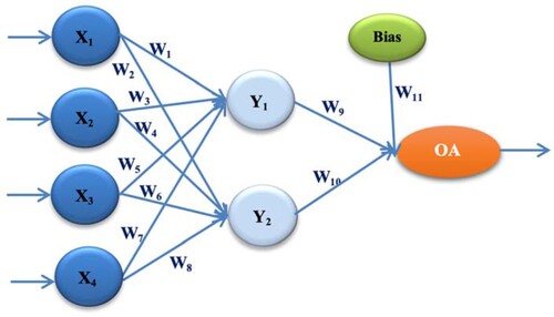
Table 1. Taguchi Orthogonal Array (L12 = 2¹¹).

ANN-L12	W1	W2	W3	W4	W5	W6	W7	W8	W9	W10	W11
ANN1	L1	L1	L1	L1	L1	L1	L1	L1	L1	L1	L1
ANN2	L1	L1	L1	L1	L1	L2	L2	L2	L2	L2	L2
ANN3	L1	L1	L2	L2	L2	L1	L1	L1	L2	L2	L2
ANN4	L1	L2	L1	L2	L2	L1	L2	L2	L1	L1	L2
ANN5	L1	L2	L2	L1	L2	L2	L1	L2	L1	L2	L1
ANN6	L1	L2	L2	L2	L1	L2	L2	L1	L2	L1	L1
ANN7	L2	L1	L2	L2	L1	L1	L2	L2	L1	L2	L1
ANN8	L2	L1	L2	L1	L2	L2	L2	L1	L1	L1	L2
ANN9	L2	L1	L1	L2	L2	L2	L1	L2	L2	L1	L1
ANN10	L2	L2	L2	L1	L1	L1	L1	L2	L2	L1	L2
ANN11	L2	L2	L1	L2	L1	L2	L1	L1	L1	L2	L2
ANN12	L2	L2	L1	L1	L2	L1	L2	L1	L2	L2	L1

The second proposed architecture is ANN-L36prim. It consists of 4 input values, one hidden layer with three nodes, one output, and the total number of 16 weighting factors W_i(i =$\overline{(1,16)}$, whose initial values are from the interval [−1, 0, 1]. The Taguchi Orthogonal Array used in the construction of this proposed architecture is combined, where the first 11 parameters and the last 16th parameter are with three levels L1, L2, and L3, while the remaining four parameters are with two levels L1 and L2 Figure 2, Table 2 (N. Rankovic et al., 2021; Stoica & Blosiu, 1997).

Figure 2. ANN architecture with a single hidden layer (ANN-L36prim).

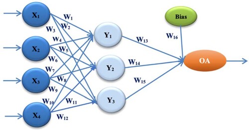
Table 2. Taguchi Orthogonal Array (L36prim = 3¹¹2⁴3¹).

ANN-L36	W1	W2	W3	W4	W5	W6	W7	W8	W9	W10	W11	W12	W13	W14	W15	W16
ANN1	L1	L1	L1	L1	L1	L1	L1	L1	L1	L1	L1	L1	L1	L1	L1	L1
ANN2	L2	L2	L2	L2	L2	L2	L2	L2	L2	L2	L2	L2	L1	L1	L1	L1
ANN3	L3	L3	L3	L3	L3	L3	L3	L3	L3	L3	L3	L3	L1	L1	L1	L1
ANN4	L1	L1	L1	L1	L2	L2	L2	L2	L3	L3	L3	L3	L1	L2	L2	L1
ANN5	L1	L1	L1	L1	L3	L3	L3	L3	L2	L2	L2	L2	L1	L2	L2	L1
ANN6	L3	L3	L3	L3	L1	L1	L1	L1	L2	L2	L2	L2	L1	L2	L2	L1
ANN7	L1	L1	L2	L3	L1	L2	L3	L3	L1	L1	L1	L3	L2	L1	L2	L1
ANN8	L2	L2	L3	L1	L2	L3	L1	L1	L2	L3	L3	L1	L2	L1	L2	L1
ANN9	L3	L3	L1	L2	L3	L1	L2	L2	L3	L1	L1	L2	L2	L1	L2	L1
ANN10	L1	L1	L3	L2	L1	L3	L2	L3	L2	L1	L3	L2	L2	L2	L1	L1
ANN11	L2	L2	L1	L3	L2	L1	L3	L1	L3	L2	L1	L3	L2	L2	L1	L1
ANN12	L3	L3	L2	L1	L3	L2	L1	L2	L1	L3	L2	L1	L2	L2	L1	L1
ANN13	L1	L2	L3	L1	L3	L2	L1	L3	L3	L2	L1	L2	L1	L1	L1	L2
ANN14	L2	L3	L1	L2	L1	L3	L2	L1	L1	L3	L2	L3	L1	L1	L1	L2
ANN15	L3	L1	L2	L3	L2	L1	L3	L2	L2	L1	L3	L1	L1	L1	L1	L2
ANN16	L1	L2	L3	L2	L1	L1	L3	L2	L3	L3	L2	L1	L1	L2	L2	L2
ANN17	L2	L3	L1	L3	L2	L2	L1	L3	L1	L1	L3	L2	L1	L2	L2	L2
ANN18	L3	L1	L2	L1	L3	L3	L2	L1	L2	L2	L1	L3	L1	L2	L2	L2
ANN19	L1	L2	L1	L3	L3	L3	L1	L2	L2	L1	L2	L3	L2	L1	L2	L2
ANN20	L2	L3	L2	L1	L1	L1	L2	L3	L3	L2	L3	L1	L2	L1	L2	L2
ANN21	L3	L1	L3	L2	L2	L2	L3	L1	L1	L3	L1	L2	L2	L1	L2	L2
ANN22	L1	L2	L2	L3	L3	L1	L2	L1	L1	L3	L3	L2	L2	L2	L1	L2
ANN23	L2	L3	L3	L1	L1	L2	L3	L2	L2	L1	L1	L3	L2	L2	L1	L2
ANN24	L3	L1	L1	L2	L2	L3	L1	L3	L3	L2	L2	L1	L2	L2	L1	L2
ANN25	L1	L3	L2	L1	L2	L3	L3	L1	L3	L1	L2	L2	L1	L1	L1	L3
ANN26	L2	L1	L3	L2	L3	L1	L1	L2	L1	L2	L3	L3	L1	L1	L1	L3
ANN27	L3	L2	L1	L3	L1	L2	L2	L3	L2	L3	L1	L1	L1	L1	L1	L3
ANN28	L1	L3	L2	L2	L2	L1	L1	L3	L2	L3	L1	L3	L1	L2	L2	L3
ANN29	L2	L1	L3	L3	L3	L2	L2	L1	L3	L1	L2	L1	L1	L2	L2	L3
ANN30	L3	L2	L1	L1	L1	L3	L3	L2	L1	L2	L3	L2	L1	L2	L2	L3
ANN31	L1	L3	L3	L3	L2	L3	L2	L2	L1	L2	L1	L1	L2	L1	L2	L3
ANN32	L2	L1	L1	L1	L3	L1	L3	L3	L3	L3	L2	L2	L2	L1	L2	L3
ANN33	L3	L2	L2	L2	L1	L2	L1	L1	L3	L1	L3	L3	L2	L1	L2	L3
ANN34	L1	L3	L1	L2	L3	L2	L3	L1	L2	L2	L3	L1	L2	L2	L1	L3
ANN35	L2	L1	L2	L3	L1	L3	L1	L2	L3	L3	L1	L2	L2	L2	L1	L3
ANN36	L3	L2	L3	L1	L2	L1	L2	L3	L1	L1	L2	L3	L2	L2	L1	L3

The experiment presented in this paper consists of three parts:

1. Training of two different ANN architectures constructed according to the corresponding Taguchi Orthogonal Plans (ANN-L12 and ANN36prim);

2. Testing on ANN, which gave the best results (the lowest MMRE value) in the 1st part of the experiment, for two proposed architectures on the same dataset;

3. Validation on ANN, which gave the best results (the lowest MMRE value) in the 1st part of the experiment, for each selected architecture, but using some other i.e. different datasets.

For the first and second part of the experiment, the ISBSG of industrial projects (2015) repository was used. In contrast, in the third part, the Desharnais dataset and a combined dataset composed of projects of different companies were used. ISBSG offers a wealth of information regarding practices from various organisations, applications, and development types, constituting its main potential. The ISBSG suggests that the most important criteria for estimation purposes are the functional size; the development type (new development, enhancement, or re-development); the primary programming language or the language type/generation (e.g. 3GL, 4GL); and the development platform (mainframe, midrange or PC). The results in Table 3. indicate the heterogeneous nature of the designs of each dataset used and within all three parts of the experiment. It can be seen that data sets are very different in terms of the programming languages used, the duration of application development, and an extensive range of functional size values, with a large standard deviation Table 4.

Table 3. Information on used datasets.

	Datasets	Number of project	Experiment
Dataset_1	ISBSG (Functional Size<10)	37	Training
	ISBSG (Functional Size<10)	15	Testing
Dataset_2	ISBSG (10<Functional Size<50)	45	Training
	ISBSG (10<Functional Size<50)	17	Testing
Dataset_3	ISBSG (50<Functional Size<100)	30	Training
	ISBSG (10<Functional Size<100)	13	Testing
Dataset_4	ISBSG (100<Functional Size<500)	60	Training
	ISBSG (10<Functional Size<500)	17	Testing
Datset_5	ISBSG (Functional Size>500)	14	Training
	ISBSG (Functional Size>500)	7	Testing
Dataset_6	Desharnais	14	Validation1
Dataset_7	Combined	33	Validation2

Table 4. Basic statistics about datasets.

Datasets	N	Min [PM]	Max [PM]	Mean [PM]	Std. deviation [PM]
Dataset_1	52	2.0	9.0	5.404	2.4031
Dataset_2	62	10.0	48.0	24.823	11.3203
Dataset_3	43	50.0	99.0	77.116	15.1441
Dataset_4	77	104.0	492.0	234.130	113.8159
Dataset_5	21	561.0	2090.0	1016.048	458.4442
Dataset_6	14	140.0	3860.0	1011.429	920.4251
Dataset_7	33	493.0	2589.0	1193.424	419.4201

3.2. Robust design of the experiment

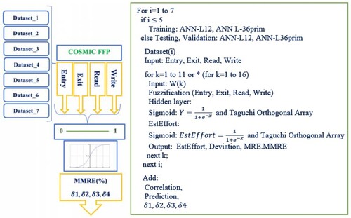
The first part of the experiment involves training two selected ANN architectures and consists of the following steps:

1. Input values are the data about particular project from the selected ISBSG dataset and are represented by four parameters (Entry, Exit, Read, Write), which describe the functional size.

2. All input values are transformed according to the following formula: The function μD(X):R → [0, 1], translates the real values of input signals into coded values from the interval [0, 1], in the following way (Chhabra & Singh, 2020; Kataev et al., 2020): μD(X_i) = (X_i − X_min)/(X_max − X_min), where D is the set of data on which the experiment is performed, X_i is the input value, X_min is the smallest input value, and X_max the greatest input value on the observed dataset.

3. The sigmoid function, as the activation function of the hidden layer was used: $y=\frac{1}{1+e^{-X_i}},\mathbf{\text{i}}=(\overline{1,n})$The construction of the activation function is based on a combination of input values and corresponding weight factors W_i for each of the listed ANN architectures.

Hidden and output layer functions for ANN-L12 architecture: $\begin{array}{rl}Y1& =\frac{1}{1+e^{-(X1\cdot W1+X2\cdot W3+X3\cdot W5+X4\cdot W7)}}\\ Y2& =\frac{1}{1+e^{-(X1\cdot W2+X2\cdot W4+X3\cdot W6+X4\cdot W8)}}\\ EstEffort& =\frac{1}{1+e^{-(Y1\cdot W9+Y2\cdot W10+1\cdot W11)}}\end{array}$

Where Y1 and Y2 are the hidden layer functions and EstEffort represents output function.

Hidden and output layer functions for ANN-L36prim architecture: $\begin{array}{rl}Y1& =\frac{1}{1+e^{-(X1\cdot W1+X2\cdot W4+X3\cdot W7+X4\cdot W10)}}\\ Y2& =\frac{1}{1+e^{-(X1\cdot W2+X2\cdot W5+X3\cdot W8+X4\cdot W11)}}\\ Y3& =\frac{1}{1+e^{-(X1\cdot W3+X2\cdot W6+X3\cdot W9+X4\cdot W12)}}\\ EstEffort& =\frac{1}{1+e^{-(Y1\cdot W13+Y2\cdot W14+Y3\cdot W15+1\cdot W16)}}\end{array}$

Where Y1, Y2, and Y3 are the hidden layer functions and EstEffort represents output function.

In the first proposed ANN-L12 architecture, an Orthogonal plan of two levels L1 and L2, and the initial values of the weighting factors W_i that take the values from the interval [−1, 1], were used. The second proposed architecture has an Orthogonal plan of three levels L1, L2, and L3, and the initial values of the weighting factors Wi that take the values from the interval [−1, 0, 1]. For each subsequent iteration, new weight factor values must be calculated as follows (e.g. for ANN-L12 architecture) (Khaw et al., 1995; Stoica & Blosiu, 1997): $\begin{array}{rl}{W}_1\cdot L1& =cost1+cost2+\dots +cost6\\ W_1\cdot L2& =cost7+cost8+...+cost12\\ & \dots \\ W_{12}\cdot L1& =cost1+cost5+\dots +cost12\\ W_{12}\cdot L2& =cost2+cost3+\dots +cost11\end{array}$where cost(i) = Σ M RE(ANN(i))

For each subsequent iteration, the interval [−1, 1] is divided depending on the cost effect function as follows: $\begin{array}{rl}{W}_1\cdot L1new& =W_1\cdot L1old\\ W_1\cdot L2new& =W_1\cdot L2old+(W_1\cdot L2old-W_1\cdot L1old)/2\end{array}$where W₁·L1old and W₁·L2old are values form the previous iteration. The set of input values of each dataset converges depending on the value of the cost effect function.

4. Method of defuzzification was used according to the following formula:

Xi = (X_min + μD(X_i)) · (X_max − X_min)

OA(ANNi) = Xi, where i = 12, i = 36.

Where OA represents actual effort of the particular project, that is calculated based on ANN-L12 and ANN-L36prim.

5. For each iteration in our experiment, the output values are obtained according to the following formulas/measures (N. Rankovic et al., 2021):

Deviation = ABS (Actual_Effort – Estimated_Effort)

MRE = Deviation/Actual_Effort

MRE = 1 n · ∑ MREi n i=1 and MMRE = mean (MRE)

For each experimental part in each iteration, the Gradient Descent (GA) with the condition GA< 0.01, where i = $\overline{1,n}$; for n = $\overline{1,12}$ or n = $\overline{1,36}$; n is a number of ANN monitored (N. Rankovic et al., 2021).

6. Examination of the influence of input values on the change of MMRE values:

1. The influence of the first input parameter (Entry) and his value is calculated as:

   δ₁ = mean(MMRE) – mean(MMRE₁)

   where MMRE₁ is mean(MMRE) when X₁=0;

2. The influence of the second input parameter (Exit) and his value is calculated as:

   δ₂ = mean(MMRE) – mean(MMRE₂)

   where MMRE₂ is mean(MMRE) when X₂=0;

3. The influence of the third input parameter (Read) and his value is calculated as:

   δ₃ = mean(MMRE) – mean(MMRE₃)

   where MMRE₃ is mean(MMRE) when X₃=0;

4. The influence of the fourth input parameter (Write) and his value is calculated as:

   δ₄ = mean(MMRE) – mean(MMRE₄)

   where MMRE₄ is mean(MMRE) when X₄=0;

7. Prediction at 25%, 30%, and 50% is the percentage of the total number of ANNs that meet the GA criterion. $PRED(x)\frac{1}{n}\cdot \sum _{i=1}^n\{\begin{array}{l}1,ifMRE\le x\\ 0,otherwise\end{array}$

PRED(k) = count(MRE) < 25%

PRED(k) = count(MRE) < 30%

PRED(k) = count(MRE) < 50%, where k = 25, k = 30, and k = 50.

Additionally, the Pearson (Kataev, 2020) and Spearman’s correlation (Chhabra & Singh, 2020) coefficients are monitored.

The second and third parts are executed by the same algorithm as the first part, with different projects and datasets. The second part uses the ISBSG dataset, but with projects that were not used in the first part. In the third part, the Desharnais dataset and combined dataset are used.

The robust design of the experiment can be represented graphically as follows in Figure 3.

Figure 3. Robust design of experiment.

4. Discussion

The proposed methodology in this paper involves selecting the most straightforward architecture depending on the number of input values. The ANN network architecture includes input values, none or more hidden layers, and an output layer. The shape, type, and size of ANN training parameters affect the specific ANN architecture. In constructing all the proposed architectures, the Taguchi Orthogonal Array to optimise the design parameters was used. In ANN design that uses the Taguchi methodology, the engineer must investigate the application problem well. The advantage of this approach over other non-parametric models is based on estimating any function with optional precision. To simplify optimisation problems, in the paper, we use various Taguchi Orthogonal Arrays representing the MFFN (Multilayer Feed Forward Neural Network) class, which has a vital role in solving different types of problems in science, engineering, medicine, pattern recognition, nuclear sciences, and other fields (Stoica & Blosiu, 1997). No clearly defined theory allows the calculation of ideal parameter settings to construct a high-performance MFFN. This leads to the conclusion that even small changes in parameters can cause significant differences in the behaviour of almost all networks. In (Khaw et al., 1995), an analysis of Neural network design factors and object functions is given, in which an architecture with one or two hidden layers is recommended. We start experimenting with the simple ANN architectures. In our approach, the first proposed ANN-L12 architecture with one hidden layer and two nodes, and then the second proposed ANN-L36prim architecture with one hidden layer and three nodes. The number of hidden layers indicates reducing the number of iterations to achieve the stop criteria. Our choice of ANN architecture with one hidden layer did not significantly increase the number of factors. In the ANN-L12 architecture, this number is 11, and in the ANN-L36prim is 16, which was acceptable in our study, while our experiments showed that the MMRE value was reduced by 0.9%. It is unnecessary to introduce more complex architectures because this did not require more processor processing than other ANN architects we experimented with.

The result we monitor during the execution of the required iterations is the value of MMRE, which, depending on the nature of the dataset, proved to be stable for the two proposed architectures in all three parts of the experiment. Datasets with a small functional size have a higher value of MMRE (Dataset_1, Dataset_2) than datasets with a medium value of functional size (Dataset_3). Datasets with a large functional size value have a mean MMRE value (Dataset_4, Dataset_5). Validation datasets have different values of functional magnitude and have a higher MMRE value. The lowest value of MMRE is achieved on Dataset_3 for the proposed ANN-L12 architecture (17.0%), while for ANN-L36prim the value of MMRE is 16.4%. The mean MMRE value on all datasets in all three parts of the experiment was 29.7% for ANN-L12 and 28.8% for ANN-L36prim Figure 4, Table 5. Compared to the COCOMO approach, presented in [4], the value of MMRE was significantly reduced by 14.5% Table 6.

Figure 4. Graphical representation of MMRE value for each proposed ANN architecture.

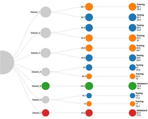
Table 5. MMRE value for each proposed ANN architecture.

Datasets	ANN-L12 MMRE(%)	ANN-L36prim MMRE(%)	Part of experiment
Dataset_1	36.1	36.2	Training
	36.7	35.6	Testing
Dataset_2	33.2	32.0	Training
	36.6	33.8	Testing
Dataset_3	17.0	16.4	Training
	18.1	17.2	Testing
Dataset_4	29.6	29.7	Training
	29.8	29.6	Testing
Dataset_5	24.2	19.0	Training
	27.0	24.8	Testing
Dataset_6	34.9	39.1	Validation1
Dataset_7	33.2	31.8	Validation2
AVERAGE(MMRE)	29.7	28.8

Table 6. COCOMO vs. COSMIC FP.

COCOMO model			Functional point – COSMIC model
ANN L-18 MMRE (%)	ANN L-27 MMRE (%)	ANN L-36 MMRE (%)	ANN L-12 MMRE (%)	ANN L-36prim MMRE (%)
59.7	45.3	43.3	29.7	28.8

The correlation coefficient is a measure of the agreement of two quantities. The higher the value of the correlation coefficient, the more stable the relationship between the observed values. By calculating the correlation coefficient between the estimated and actual value, the proposed approach's reliability, accuracy, and precision can be determined. Correlation coefficients, calculated according to Pearson and Spearman, indicate that the correlation is very high. The best result is achieved on Dataset_2 and Dataset_4, while the worst outcome is achieved on Dataset_6 and Dataset_7 Table 7.

Table 7. Correlation coefficients.

Correlation	Pearson		Spearman's rho
Datasets	ANN-L12	ANN-L36prim	ANN-L12	ANN-L36prim
Dataset_1	0.859	0.756	0.884	0.785
Dataset_2	0.984	0.788	0.984	0.808
Dataset_3	0.734	0.688	0.745	0.678
Dataset_4	0.912	0.911	0.918	0.917
Dataset_5	0.767	0.618	0.715	0.918
Dataset_6	0.628	0.586	0.612	0.534
Dataset_7	0.674	0.622	0.654	0.618

Prediction is one of the criteria used to confirm the accuracy of the proposed estimation approach. By monitoring the prediction at three different values: 25%, 30%, and 50%, it is possible to conclude the appropriate degree of certainty of the proposed approach. This allows the best model of the presented ANN architectures to be selected. If the prediction value is high, the proposed model is good. In our approach, the highest prediction value on the 25% criterion is achieved on the Dataset_3 ANN-L36prim architecture (84.1%). The highest prediction value on the 30% criterion is conducted on the Dataset_3 ANN-L36prim architecture (86.4%). The prediction value on the 50% criterion is achieved again for the ANN-L36prim architecture but within the Dataset_1 (98.1%). We can show that in our work, prediction represents the percentage of projects that have an MRE value of less than 25%, 30, and 50%, respectively Table 8.

Table 8. Prediction measured on three criterions.

PRED (%)	P(25)		P(30)		P(50)
Datasets	ANN-L12	ANN-L36prim	ANN-L12	ANN-L36prim	ANN-L12	ANN-L36prim
Dataset_1	39.6	37.7	49.1	52.8	83.0	98.1
Dataset_2	33.3	31.7	41.3	44.4	69.8	82.5
Dataset_3	79.5	84.1	86.4	86.4	95.5	97.7
Dataset_4	42.3	42.3	51.3	51.3	78.2	80.8
Dataset_5	50.0	59.1	54.5	63.6	81.8	86.4
Dataset_6	28.6	28.6	28.6	35.7	78.6	78.6
Dataset_7	30.3	30.3	42.4	57.6	81.8	84.8

In addition to the known criteria for monitoring the efficiency, effectiveness, and precision of the proposed approach, the influence of the input values of the COSMIC FP method on the change in the MMRE value was also monitored. By omitting each value for the four input values (Entry, Exit, Read, and Write), the change in MMRE versus mean (MMRE) for the proposed architecture on each selected dataset was monitored. In this way, it is possible to determine the impact of each input value on the final estimated value of the project.

When examining the influence of these input values for the ANN-L12 architecture, it can be concluded that the most significant influence has the second input value (Exit) in Dataset_1 (5.3%) and the smallest first input value (Entry) on Dataset_6 (−1.1%). It can be concluded that the Exit value in Dataset_1 increases the MMRE value by 5.3%, while Entry decreases the MMRE value by 1.1%. The influence of all four input values on all seven datasets ranges to the interval [−1.1, 5.3]. A value of 0.0% means that the input value does not affect the change in the MMRE value Figure 5, Table 9.

Figure 5. Graphical representation of the influence of input values on MMRE value (ANN-L12 architecture).

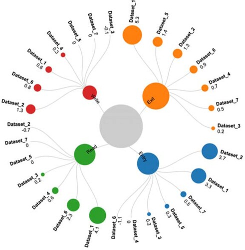
Table 9. Influence of input values on MMRE value (δ(%)) – ANN-L12 architecture.

δ(%)	Dataset_1	Dataset_2	Dataset_3	Dataset_4	Dataset_5	Dataset_6	Dataset_7
Entry	3.3	3.7	0.2	0.0	0.3	−1.1	0.5
Exit	5.3	1.3	0.2	0.7	1.4	0.9	0.5
Read	4.1	−0.7	0.2	0.6	0.0	2.3	0.0
Write	0.6	1.3	−0.1	0.3	0.0	0.8	0.0

When examining the influence of the input values for ANN-L36rpim architecture, it can be concluded that the first input value has the most significant influence (Entry) in Dataset_2 (3.7%). In comparison, the most negligible impact has the fourth input value (Write) in Dataset_7 (−2.0%). It can be concluded that the Entry value in Dataset_2 increases the MMRE value by 3.7%, while the Write value decreases the MMRE value by 2.0%. The influence of all four input values individually on all seven datasets is moving on the interval [−2.0, 3.7] Figure 6, Table 10.

Figure 6. Graphical representation of the influence of input values on MMRE value (ANN-L36prim architecture).

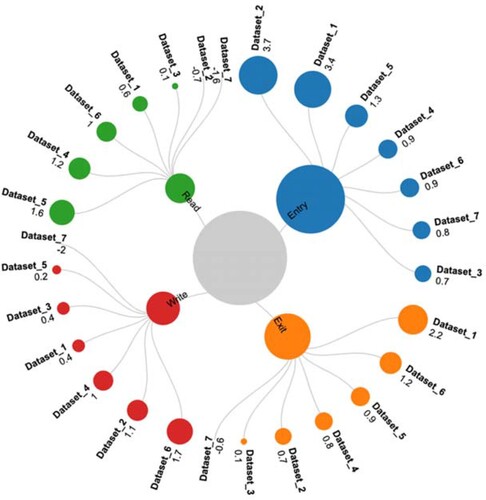
Table 10. Influence of input values on MMRE value (δ(%)) – ANN-L36prim architecture.

δ(%)	Dataset_1	Dataset_2	Dataset_3	Dataset_4	Dataset_5	Dataset_6	Dataset_7
Entry	3.4	3.7	0.7	0.9	1.3	0.9	0.8
Exit	2.2	0.7	0.1	0.8	0.9	1.2	−0.6
Read	0.6	−0.7	0.1	1.2	1.6	1	−1.6
Write	0.4	1.1	0.4	1	0.2	1.7	−2.0

The COSMIC FP measure defines a model of software functionality. By monitoring the influence of input values (Entry, Exit, Read, Write), the value of MMRE can be further improved depending on the user's needs, i.e. his functional requirements. By examining the individual effects of four different input values, it can be concluded that the most significant changes come from Entry and Exit input values. Therefore, it is necessary to re-perform the analysis and additional testing of these two input values, but they will not change the MMRE value in the estimation process. The models and tools currently used to estimate software project development efforts use functional points that express the functional size of that programme. Recent research and many companies use the COSMIC FP method because it is possible to assess the development effort in the initial stage compared to previously used FPA methods. The obtained results of the used COSMIC FP method show that it is possible with our approach and applied methodology to estimate the functional size quite accurately. Remarkably, the results found tend to suggest that in the presence of a set of projects – concerning the applying domain, the nature of computation performed, and the implementation technology – it is possible to get more accurate estimates of the functional size (expressed either in FP or in CFP) on the premise of several base functional components (BFC) (Lavazza & Liu, 2019). Before specifying the requirements specification in detail, it is possible to make an early assessment if there is not enough time to apply some other standard methods (Borandag et al., 2019; Janković et al., 2019).

5. Conclusion

The presented experiment proved that the evaluation of software projects using the COSMIC FP method and two different ANN architectures based on Taguchi Orthogonal Arrays could further minimise the value of MMRE. The COSMIC FP method belongs to a group of approaches that consider the user's functional requirements using four input values. In addition to the mentioned method, the clustering method of input values and transformations such as fuzzification of input values was used to directly and partially control the different nature of projects. The heterogeneous nature of the project is observed depending on the available input factors, i.e. measured attributes (predictors) of the software project that affect the prediction of software development efforts (ratio of minimum and maximum values on the observed set of projects). It was concluded that the models constructed of the two proposed ANN architectures (ANN-L12 and ANN-L36prim) give a significantly lower value of MMRE, which differs by 14.5% compared to the previous study conducted on different attributes of the COCOMO model (N. Rankovic et al., 2021). The obtained results show that the difference in MMRE of the more complex ANN-L36prim architecture is lower by 0.9% compared to the ANN-L12 architecture. Using two correlation coefficients, we confirmed the ratio of the observed values in the above experiment and thus demonstrated the efficiency and stability of the proposed model. Monitoring the value of prediction on three different criteria further confirmed the correctness and reliability of this approach. This paper's main goal is to decrease the MMRE and examine the influence of the input values of the used COSMIC FP method on the change of the MMRE value on each of the seven used datasets from several sources. The main advantages of the proposed approach are: 1) the small number of iterations (less than 7) – which significantly reduces execution time, 2) use of simple ANN architectures, 3) optimisation of proposed ANN architectures using Taguchi Orthogonal Arrays, 4) high coverage of different values of software projects, and 5) use of ISBSG dataset as one of the relevant sources which contain project data collected from other companies.

There are no specific limitations in our approach. It is applicable in different business areas or other fields of science such as medicine, pattern recognition, nuclear sciences, etc., not only in software engineering. The proposed approach could be used to construct a tool for adequate, rapid, and accurate assessment of the functionality required to implement software projects. This can further reduce the problems and tasks most often encountered by experts and software teams in software engineering.

Disclosure statement

No potential conflict of interest was reported by the author(s).

References

- Angara, J., Prasad, S., & Sridevi, G. (2018). Towards Benchmarking user stories estimation with COSMIC function points-A case example of participant observation. International Journal of Electrical & Computer Engineering, 8(5), 3076–3083. https://doi.org/10.11591/ijece.v8i5.pp3076-3083
- Bagriyanik, S., & Karahoca, A. (2018). Using data mining to identify COSMIC function point measurement competence. International Journal of Electrical and Computer Engineering, 8(6), 5253–5259. https://doi.org/10.11591/ijece.v8i6.pp5253-5259
- Borandag, E., Ozcift, A., Kilinc, D., & Yucalar, F. (2019). Majority vote Feature Selection algorithm in software fault prediction. Computer Science and Information Systems, 16(2), 515–539. https://doi.org/10.2298/CSIS180312039B
- CHAOS Report. (2013). The Standish Group.
- Chhabra, S., & Singh, H. (2020). Optimizing design of Fuzzy model for software cost estimation using particle swarm optimization algorithm. International Journal of Computational Intelligence and Applications, 19(1), 2050005. https://doi.org/10.1142/S1469026820500054
- Cuadrado-Gallego, J. J., Buglione, L., Rejas-Muslera, R. J., & Machado-Piriz, F. (2008, September 3–5). IFPUG-COSMIC statistical conversion. 34th Euromicro Conference Software Engineering and Advanced Applications, Parma, Italy (pp. 427–432). IEEE. https://doi.org/10.1109/SEAA.2008.75
- De Vito, G., Ferrucci, F., & Gravino, C. (2020). Design and automation of a COSMIC measurement procedure based on UML models. Software and Systems Modeling, 19(1), 171–198. https://doi.org/10.1007/s10270-019-00731-2
- Di Martino, S., Ferrucci, F., Gravino, C., & Sarro, F. (2016). Web effort estimation: Function point analysis vs. COSMIC. Information and Software Technology, 72, 90–109. https://doi.org/10.1016/j.infsof.2015.12.001
- Di Martino, S., Ferrucci, F., Gravino, C., & Sarro, F. (2020). Assessing the effectiveness of approximate functional sizing approaches for effort estimation. Information and Software Technology, 123, 106308. https://doi.org/10.1016/j.infsof.2020.106308
- Fehlmann, T., & Santillo, L. (2010, November). From story points to cosmic function points in agile software development – A six sigma perspective. Metrikon-Software Metrik Kongress (p. 24).
- Fu, T., Tang, X., Cai, Z., Zuo, Y., Tang, Y., & Zhao, X. (2020). Correlation research of phase angle variation and coating performance by means of Pearson’s correlation coefficient. Progress in Organic Coatings, 139, 105–459. https://doi.org/10.1016/j.porgcoat.2019.105459
- Goyal, S., & Parashar, A. (2018). Machine learning application to improve COCOMO model using neural networks. International Journal of Information Technology and Computer Science (IJITCS), 10(3), 35–51. https://doi.org/10.5815/ijitcs.2018.03.05
- Hussain, I., Kosseim, L., & Ormandjieva, O. (2013). Approximation of COSMIC functional size to support early effort estimation in agile. Data & Knowledge Engineering, 85, 2–14. https://doi.org/10.1016/j.datak.2012.06.005
- International Software Benchmarking Standards Group (ISBSG). (2015). ISBSG repository from https://www.isbsg.org/
- Janković, M., Žitnik, S., & Bajec, M. (2019). Reconstructing De facto software development methods. Computer Science and Information Systems, 16(1), 75–104. https://doi.org/10.2298/CSIS180226038J
- Jiang, Y., Liang, W., Tang, J., Zhou, H., Li, K. C., & Gaudiot, J. L. (2021). A novel data representation framework based on nonnegative manifold regularisation. Connection Science, 33(2), 136–152. https://doi.org/10.1080/09540091.2020.1772722
- Jiao, J., Wang, L., Li, Y., Han, D., Yao, M., Li, K. C., & Jiang, H. (2021). CASH: Correlation-aware scheduling to mitigate soft error impact on heterogeneous multicores. Connection Science, 33(2), 113–135. https://doi.org/10.1080/09540091.2020.1758924
- Kataev, M., Bulysheva, L., Xu, L., Ekhlakov, Y., Permyakova, N., & Jovanovic, V. (2020). Fuzzy model estimation of the risk factors impact on the target of promotion of the software product. Enterprise Information Systems, 14(6), 797–811. https://doi.org/10.1080/17517575.2020.1713407
- Kaur, A., & Kaur, K. (2019). A COSMIC function points based test effort estimation model for mobile applications. Journal of King Saud University-Computer and Information Sciences. https://doi.org/10.1016/j.jksuci.2019.03.001
- Khaw, J. F. C., Lim, B. S., & Lim, L. E. N. (1995). Optimal design of neural networks using the Taguchi method. Neurocomputing, 7 (30), 225–245. https://doi.org/10.1016/0925-2312(94)00013-I
- Kheyrinataj, F., & Nazemi, A. (2020). Fractional power series neural network for solving delay fractional optimal control problems. Connection Science, 32(1), 53–80. https://doi.org/10.1080/09540091.2019.1605498
- Lavazza, L., & Liu, G. (2019, November 24–28). An empirical evaluation of the accuracy of NESMA function points estimates. The Fourteenth International Conference on Software Engineering Advances (ICSEA), Valencia, Spain.
- Meng, J., Ricco, M., Luo, G., Swierczynski, M., Stroe, D. I., Stroe, A. I., & Teodorescu, R. (2017). An overview and comparison of online implementable SOC estimation methods for lithium-ion battery. IEEE Transactions on Industry Applications, 54(2), 1583–1591. https://doi.org/10.1109/TIA.2017.2775179
- Moosavi, S. H. S., & Bardsiri, V. K. (2017). Satin bowerbird optimizer: A new optimization algorithm to optimize ANFIS for software development effort estimation. Engineering Applications of Artificial Intelligence, 60, 1–15. https://doi.org/10.1016/j.engappai.2017.01.006
- Ochodek, M., Kopczyńska, S., & Staron, M. (2020). Deep learning model for end-to-end approximation of COSMIC functional size based on use-case names. Information and Software Technology, 123, 106310. https://doi.org/10.1016/j.infsof.2020.106310
- Popović, J., & Bojić, D. (2012). A comparative evaluation of effort estimation methods in the software life cycle. Computer Science and Information Systems, 9(1), 455–484. https://doi.org/10.2298/CSIS110316068P
- Potha, N., Kouliaridis, V., & Kambourakis, G. (2021). An extrinsic random-based ensemble approach for android malware detection. Connection Science, 33(4), 1077–1093. https://doi.org/10.1080/09540091.2020.1853056
- Qiu, L., Sai, S., & Tian, X. (2021). TsFSIM: A three-step fast selection algorithm for influence maximisation in social network. Connection Science, 33(4), 854–869. https://doi.org/10.1080/09540091.2021.1904206
- Quesada-López, C., Madrigal-Sánchez, D., & Jenkins, M. (2020, February). An empirical analysis of IFPUG FPA and COSMIC FP measurement methods. International Conference on Information Technology & Systems (pp. 265–274). Springer.
- Rankovic, D., Rankovic, N., Ivanovic, M., & Lazic, L. (2021). Convergence rate of artificial neural networks for estimation in software development projects. Information and Software Technology, 138, 106627. https://doi.org/10.1016/j.infsof.2021.106627
- Rankovic, N., Rankovic, D., Ivanovic, M., & Lazic, L. (2021). A new approach to software effort estimation using different artificial neural network architectures and Taguchi Orthogonal Arrays. IEEE Access, 9, 26926–26936. https://doi.org/10.1109/ACCESS.2021.3057807
- ReliaSoft Publishing. (2012, January). Taguchi Orthogonal Array Designs from https://www.weibull.com/hotwire/issue131/hottopics131.htm
- Sabaghian, A., Balochian, S., & Yaghoobi, M. (2020). Synchronisation of 6D hyper-chaotic system with unknown parameters in the presence of disturbance and parametric uncertainty with unknown bounds. Connection Science, 32(4), 362–383. https://doi.org/10.1080/09540091.2020.1723491
- Sakhrawi, Z., Sellami, A., & Bouassida, N. (2020). Investigating the impact of functional size measurement on predicting software enhancement effort using correlation-based feature selection algorithm and SVR method. In S. Ben Sassi, S. Ducasse, & H. Mili (Eds.), Reuse in emerging software engineering practices (19th International Conference on Software and Systems Reuse, ICSR 2020, Hammamet, Tunisia, Lecture notes in Computer Science, Vol. 12541, pp. 229-244). Springer. https://doi.org/10.1007/978-3-030-64694-3_14
- Salmanoglu, M., Hacaloglu, T., & Demirors, O. (2017). Effort estimation for agile software development: comparative case studies using COSMIC functional size measurement and story points. Proceedings of the 27th International Workshop on Software Measurement and 12th International Conference on Software Process and Product Measurement (IWSM Mensura ‘17). Association for Computing Machinery, New York, NY (pp. 41–49). https://doi.org/10.1145/3143434.3143450
- Stoica, A., & Blosiu, J. (1997). Neural learning using orthogonal arrays. Advances in Intelligent Systems, 41, 418–423. ISBN Print: 978-90-5199-355-4.
- Subasri, R., Meenakumari, R., Panchal, H., Suresh, M., Priya, V., Ashokkumar, R., & Sadasivuni, K. K. (2020). Comparison of BPN, RBFN and wavelet neural network in induction motor modelling for speed estimation. International Journal of Ambient Energy, 17, 1–6. https://doi.org/10.1080/01430750.2020.1817779
- Symons, C. R. (1988). Function point analysis: Difficulties and improvements. IEEE Transactions on Software Engineering, 14(1), 2–11. https://doi.org/10.1109/32.4618
- The University of York, Department of Mathematics. (2004, May). Orthogonal Arrays (Taguchi Designs) from https://www.york.ac.uk/depts/maths/tables/orthogonal.htm
- Ugalde, F., Quesada-López, C., Martínez, A., & Jenkins, M. (2020, November). A comparative study on measuring software functional size to support effort estimation in agile. CIBSE, Brazil, American Conference on Software Engineering.
- Xia, W., Capretz, L. F., Ho, D., & Ahmed, F. (2008). A new calibration for function point complexity weights. Information and Software Technology, 50(7–8), 670–683. https://doi.org/10.1016/j.infsof.2007.07.004
- Xia, W., Ho, D., & Capretz, L. F. (2015). A neuro-fuzzy model for function point calibration. WSEAS Transactions on Information Science and Applications, 5(1), 22–30.
- Younas, M., Jawawi, D. N., Ghani, I., & Shah, M. A. (2020). Extraction of non-functional requirement using semantic similarity distance. Neural Computing and Applications, 32(11), 7383–7397. https://doi.org/10.1007/s00521-019-04226-5
- Zhang, L., Lu, D., & Wang, X. (2020). Measuring and testing interdependence among random vectors based on Spearman’s $$ρ $$ ρ and Kendall’s $$τ $$ τ. Computational Statistics, 35(4), 1685–1713. https://doi.org/10.1007/s00180-020-00973-5
- https://cosmic-sizing.org/publications/early-software-sizing-with-cosmic-practitioners-guide/