A novel general kernel-based non-negative matrix factorisation approach for face recognition

Abstract

Kernel-based non-negative matrix factorisation (KNMF) is a promising nonlinear approach for image data representation using non-negative features. However, most of the KNMF algorithms are developed via a specific kernel function and thus fail to adopt other kinds of kernels. Also, they have to learn pre-image inaccurately that may influence the reliability of the method. To address these problems of KNMF, this paper proposes a novel general kernel-based non-negative matrix factorisation (GKBNNMF) method. It not only avoids pre-image learning but also is suitable for any kernel functions as well. We assume that the mapped basis images fall within the cone spanned by the mapped training data, allowing us to use arbitrary kernel function in the algorithm. The symmetric NMF strategy is exploited on kernel matrix to establish our general kernel NMF model. The proposed algorithm is proven to be convergent. The facial image datasets are selected to evaluate the performance of our method. Compared with some state-of-the-art approaches, the experimental results demonstrate that our proposed is both effective and robust.

Keywords:

• Non-negative matrix factorisation
• Kernel function
• face recognition

1. Introduction

Machine vision is a multidisciplinary technology, which requires much knowledge in different engineering areas, such as electronic engineering, optical engineering, software engineering and so on. Machine vision obtains useful information from images to establish intelligent models of the real world. While for recognizing facial images, face recognition has become an active research topic in electronic engineering. Face recognition technology is closely related to computer vision and machine learning, which is a biometric recognition technology based on the information of human face. Face recognition system uses cameras to collect facial images and then applies artificial intelligence technology to detect and recognise facial images. Dimensionality reduction and feature extraction are important in face recognition (X. Z. Liu & Ruan, 2019) because of the curse of dimensionality problem. Based on different criteria, a large number of feature learning schemes (J. H. Chen et al., 2020; Deng et al., 2011; Guillamet et al., 2002; Hancer, 2019; C. B. He et al., 2019; Hoyer, 2004; H. Lee et al., 2010; Li et al., 2001; Lin, 2014; W. X. Liu and Zheng, 2004; Nagra et al., 2020; Qian et al., 2020; Shi et al., 2012; Xu et al., 2003; Yi et al., 2017; Zafeiriou et al., 2006; Zhou and Cheung, 2021;  Z. He et al., 2011; Turk & Pentland, 1991) have been presented to represent image data in a low dimensional feature space, among which deep learning (Davari et al., 2020; Too et al., 2020; Zalpour et al., 2020) has also been widely used in face recognition. The traditional dimensionality reduction methods involve principal component analysis (PCA) (Turk & Pentland, 1991), linear discriminant analysis (LDA) (Belhumeur et al., 1997; Yu & Yang, 2001), locality preserving projections (LPP) (X. He, 2003), wavelet transform (Akbarizadeh, 2012; Tirandaz & Akbarizadeh, 2015; Tirandaz et al., 2020) and non-negative matrix factorisation (NMF) (D. D. Lee, 1999; D. D. Lee & Seung, 2001), etc. PCA aims to find a projection matrix such that the projected data preserve the maximum distribution and have uncorrelated features simultaneously. The goal of LDA is to make use of data label information such that the data have maximum ratio of inter-scatter to intra-scatter in a low dimensional feature space. LPP algorithm keeps the inherent local structure of the data after dimensionality reduction. However, PCA, LDA and LPP algorithms usually extract features containing negative elements, which are not interpretable in face recognition due to the non-negativity of the facial images. NMF, which does not allow subtract operation, is able to acquire the parts-based representation under the non-negativity constraint. NMF algorithm approximately decomposes the non-negative data matrix into the product of two non-negative matrices, so it can extract non-negative sparse features (Eggert & Korner, 2004). Therefore, NMF has good interpretability in face recognition.

However, the above-mentioned methods are linear feature extraction algorithms. Their performances will be degraded when dealing with nonlinearly distributed data. It is known that the kernel method is effective to tackle the nonlinear problem in pattern recognition. Therefore, the linear approaches PCA, LDA, LPP and NMF are extended to their kernel counterparts KPCA (Schökopf et al., 1998), KLDA (Pekalska & Haasdonk, 2009), KLPP (Cheng et al., 2005) and KNMF (Zafeiriou & Petrou, 2010), respectively. This paper focuses on kernel-based NMF methods. The basic idea of kernel NMF is to map all image data into a kernel space through a nonlinear mapping. The mapped data can be represented as linear combinations of the mapped basis images with non-negative coefficients. Different kernel functions result in different kernel NMF algorithms, such as polynomial non-negative matrix factorisation (PNMF) (Buciu et al., 2008), quadratic polynomial kernel non-negative matrix factorisation (PKNMF) (Zhu et al., 2014), RBF kernel non-negative matrix factorisation (KNMF-RBF) (W. S. Chen et al., 2017), fractional power inner product kernel non-negative matrix factorisation (FPKNMF) (W. S. Chen et al., 2019), self-constructed cosine kernel non-negative matrix factorisation (CKNMF) (W. S. Chen et al., 2020) and so on. Empirical results on face recognition have shown that these kernel-based NMF algorithms outperform traditional linear NMF methods. Nevertheless, these kernel-based NMF methods mainly have two drawbacks, namely non-universal use of kernels and inaccurate pre-image learning. Usually, one KNMF algorithm has its own kernel, which does not work for the other kernels. For pre-image learning, these methods retain the first three terms of Taylor expansion and discard the rest terms directly. Therefore, the step of pre-image learning has a large error, which may negatively affect the performance of the algorithm. To solve these problems, Zhong et al. proposed a general NMF algorithm (GNMF) with a flexible kernel (Zhang & Liu, 2009). But GNMF algorithm still has some disadvantages. GNMF must utilise the inverse of the square root of the kernel matrix. It is known that the kernel matrix is just a positive semi-definite matrix and it is not necessarily reversible. This means that the GNMF algorithm may cause an ill-posed problem of computation. Especially, the GNMF algorithm cannot guarantee the non-negativity of the feature matrix since the inverse matrix may contain negative elements. Besides, GNMF employs eigenvalue decomposition of the kernel matrix, then directly sets the negative entries to zero. This procedure gives rise to a large decomposition error and thus affects its accuracy in classification tasks.

To sum up, most of the KNMF algorithms are developed using a specific kernel function, which limits the use of other kernels. Moreover, these methods have to learn pre-images inaccurately. These limitations may lead to unsatisfactory performance of KNMF algorithms in face recognition. In this paper, we come up with a novel general kernel-based non-negative matrix factorisation (GKBNNMF) method. It not only avoids pre-image learning but also is suitable for any kernel functions as well. We assume that the mapped basis images can be non-negatively combined by the mapped training data, allowing us to use any kernel function in the algorithm. Then we establish GKBNNMF model via symmetric NMF strategy. Our GKBNNMF model is converted to two sub-convex optimisation problems. Employing the gradient descent method, we solve the optimisation problems and obtain the update rules of GKBNNMF. To prove the convergence of the GKBNNMF algorithm, we construct a new function according to the objective function and theoretically show that the constructed function is an auxiliary function. The iterative formulas of GKBNNMF can also be derived by finding the stationary point of the auxiliary function, which implies the convergence of the proposed GKBNNMF algorithm. Our method is applied to face recognition. Three publicly available face databases, namely ORL, Caltech 101 and JAFFE databases, are chosen for evaluations. We use three kernels, polynomial kernel, RBF kernel and fractional power inner product kernel, in our GKBNNMF algorithms. Compared with the state-of-the-art kernel-based NMF approaches, our methods have competitive performance. Our method can be also applied to the other nonnegative feature extraction problems in pattern recognition. For examples, some sources must be either zero or positive to be physically meaningful in source-separation problems (Martinez & Bray, 2003), the amount of pollutant emitted by a factory is nonnegative (Paatero & Tapper, 1994), the probability of a particular topic appearing in a linguistic document is nonnegative (Novak & Mammone, 2001) and note volumes in musical audio are nonnegative (Plumbley et al., 2002). Therefore, our method is also suitable to these applications. The novelty and contributions of our paper are highlighted as follows.

• Our method can make use of arbitrary kernel functions, while previous kernel-based NMF methods can only use specific kernels. Therefore, our method has more applicability. For example, in a scenario that several sources of data are available, we can use multiple kernels in our method to combine the multiple sources.

• Our method can avoid inaccurately pre-image learning, which reduces the errors in the computations. Therefore, our method improves the reliability of kernel-based NMF methods.

• The empirical results on face recognition indicate that our method is effective when using different kernels and also robust to Gaussian noise and speckle noise.

The remainder of this paper is organised as follows. Section 2 briefly introduces the NMF-based methods, including linear and nonlinear methods. In Section 3, we present GKBNNMF approach in detail. The experimental results are reported in Section 4. Finally, the conclusion is drawn in Section 5.

2. Related work

This section will introduce the related work. The details are as follows.

2.1. NMF

NMF (D. D. Lee & Seung, 2001) is a non-negative feature extraction method for part-based representation. NMF is to approximately decompose the non-negative data matrix $X\in R_{+}^{m\times n}$ into two non-negative factors, called the basis image matrix $W\in R_{+}^{m\times r}$ and the coefficient matrix $H\in R_{+}^{r\times n}$. NMF solves the following optimisation problem: $\underset{W,H}{min}F(W,H)\mathrm{s}.\mathrm{t}.W\ge 0,H\ge 0,$where $F(W,H)$ is the objective function defined by $F(W,H)=\frac{1}{2}\parallel X-WH{\parallel }_F^2$. We can convert the above problem to two sub-convex optimisation problems and solve the problems using gradient descent method. The update rules are then acquired below: (1) $\begin{array}{rl}{H}^{(t+1)}& =H^{\left(t\right)}\otimes \frac{W^{T}X}{W^{T}W{H}^{\left(t\right)}},\\ W^{(t+1)}& =W^{\left(t\right)}\otimes \frac{X{H}^T}{W^{\left(t\right)}H{H}^T},\\ W^{(t+1)}& =\frac{W^{(t+1)}}{C},\end{array}$(1) where $C=(c_{ij}{)}_{m\times r}$ with $c_{ij}=\sum _k{w}_{kj}^{(t+1)}$. The formula (1(1) $\begin{array}{rl}{H}^{(t+1)}& =H^{\left(t\right)}\otimes \frac{W^{T}X}{W^{T}W{H}^{\left(t\right)}},\\ W^{(t+1)}& =W^{\left(t\right)}\otimes \frac{X{H}^T}{W^{\left(t\right)}H{H}^T},\\ W^{(t+1)}& =\frac{W^{(t+1)}}{C},\end{array}$(1) ) is to normalise the columns of the matrix W such that the sum of each column equals 1. $A\otimes B$ and $\frac{A}{B}$ stand for the element-wise multiplication and division between A and B, respectively.

2.2. PNMF

NMF algorithm is a linear method, thus it cannot handle nonlinear problems. To deal with nonlinear problems, PNMF (Buciu et al., 2008) algorithm has been proposed recently. PNMF extends NMF via kernel method. The idea of kernel method is to map the samples from the original space to a high-dimensional linear space by a nonlinear function ϕ, so that the mapped samples are linearly separable in the high-dimensional feature space. The polynomial kernel function is defined as follows: $k(x,y)=〈\varphi \left(x\right),\varphi \left(y\right)〉={〈x_i,x_j〉}^d,$ where $d\in N^{+}$.

First, the data matrix $X=[x_1,x_2,\dots ,x_n]\in R_{+}^{m\times n}$ in the original space is mapped to $\varphi \left(X\right)=\left[\varphi \right(x_1),\varphi (x_2),\dots ,\varphi (x_n\left)\right]$ by the nonlinear function ϕ. Then, the mapped data in the high-dimensional feature space is decomposed by NMF, i.e.$\varphi \left(X\right)\approx \varphi \left(W\right)H$, where $\varphi \left(W\right)=\left[\varphi \right(w_1),\varphi (w_2),\dots ,\varphi (w_r\left)\right]$. We define two kernel matrices: $K_{XW}=\varphi \left(X{)}^T\varphi \right(W),$and $K_{WW}=\varphi \left(W{)}^T\varphi \right(W).$The optimisation problem of PNMF is $\underset{W,H}{min}\frac{1}{2}\parallel \varphi \left(X\right)-\varphi \left(W\right)H{\parallel }_F^2,\mathrm{s}.\mathrm{t}.W\ge 0,H\ge 0.$The update rules of W and H are as follows: (2) $\begin{array}{rl}{H}^{(t+1)}& =H^{\left(t\right)}\otimes \frac{K_{WX}^{\left(t\right)}}{K_{WW}^{\left(t\right)}{H}^{\left(t\right)}},\\ W^{(t+1)}& =W^{\left(t\right)}\otimes \frac{X{K}_{XW}^{{}^{\prime }\left(t\right)}}{W\mathrm{\Lambda }{K}_{WW}^{{}^{\prime }\left(t\right)}},\\ W^{(t+1)}& =\frac{W^{(t+1)}}{C},\end{array}$(2) where $C=(c_{ij}{)}_{m\times r}$ is a matrix with $c_{ij}=\sum _k{w}_{kj}^{(t+1)}$, and Λ is a diagonal matrix with ${\mathrm{\Lambda }}_{jj}=\sum _{i=1}^n{H}_{ji}^{(t+1)}$.

3. The proposed GKBNNMF approach

To overcome the limitation of existing KNMF methods, we propose a new KNMF algorithm with a general kernel (GKBNNMF). Assuming that the basis vectors are represented as a linear combination of training data, we give a new optimisation problem of nonlinear NMF. Any type of kernel function can be used in the algorithm by replacing the kernel function with the corresponding kernel matrix. Then we derive the update rules of the optimisation problem. The convergence analysis of GKBNNMF is discussed as well.

Let the non-negative data matrix be $X=[x_1,x_2,\dots ,x_n]\in R_{+}^{m\times n}$, and the mapped data matrix be $\varphi \left(X\right)=\left[\varphi \right(x_1),\varphi (x_2),\dots ,\varphi (x_n\left)\right]$ associated with a nonlinear mapping ϕ. The inner product between x and y in the feature space can be represented by a kernel function $k(x,y)=〈\varphi \left(x\right),\varphi \left(y\right)〉$. KNMF finds non-negative matrices W and H such that $\varphi \left(X\right)\approx \varphi \left(W\right)H$. The dimensionality of $\varphi \left(X\right)$ is often very high or even infinite. Therefore, it is infeasible to decompose $\varphi \left(X\right)$ directly. We can resolve this problem in the following way. The basis vector $\varphi \left(w_i\right)$ is represented as a linear combination of $\varphi \left(x_1\right),\varphi \left(x_2\right),\dots ,\varphi \left(x_n\right)$, that is, $\varphi \left(w_i\right)=\sum _{j=1}^n{A}_{ji}\varphi \left(x_j\right)=\varphi \left(X\right)A_{.i}(i=1,2,\dots ,r)$, where $A_{.i}$ is the ith column of a non-negative matrix A. Let $\varphi \left(W\right)=\varphi \left(X\right)A$. Then we present the following cost function: (3) $\begin{array}{rl}F(W,H)& =\frac{1}{2}\parallel \varphi \left(X\right)-\varphi \left(W\right)H{\parallel }_F^2=\frac{1}{2}\parallel \varphi \left(X\right)-\varphi \left(X\right)AH{\parallel }_F^2\\ & =\frac{1}{2}\mathrm{t}\mathrm{r}(K-2KAH+H^T{A}^{T}KAH),\end{array}$(3) where $K={\varphi }^T\left(X\right)\varphi \left(X\right)$ is the kernel matrix upon X and $H\ge 0$. In (3(3) $\begin{array}{rl}F(W,H)& =\frac{1}{2}\parallel \varphi \left(X\right)-\varphi \left(W\right)H{\parallel }_F^2=\frac{1}{2}\parallel \varphi \left(X\right)-\varphi \left(X\right)AH{\parallel }_F^2\\ & =\frac{1}{2}\mathrm{t}\mathrm{r}(K-2KAH+H^T{A}^{T}KAH),\end{array}$(3) ), we convert the variable W to A. By changing the variable, we can use any kernel function avoiding the problem of the non-negativity of W.

We further simplify the objective function (3(3) $\begin{array}{rl}F(W,H)& =\frac{1}{2}\parallel \varphi \left(X\right)-\varphi \left(W\right)H{\parallel }_F^2=\frac{1}{2}\parallel \varphi \left(X\right)-\varphi \left(X\right)AH{\parallel }_F^2\\ & =\frac{1}{2}\mathrm{t}\mathrm{r}(K-2KAH+H^T{A}^{T}KAH),\end{array}$(3) ). Since K is a symmetric semi-positive definite matrix and $K={\varphi }^T\left(X\right)\varphi \left(X\right)$, we can find $\varphi \left(X\right)$ by symmetric nonnegative matrix factorisation (SNMF). Apply SNMF to K, that is, $K\approx S{S}^T$ with $S\in R^{n\times k}$ and $S\ge 0$. Then (3(3) $\begin{array}{rl}F(W,H)& =\frac{1}{2}\parallel \varphi \left(X\right)-\varphi \left(W\right)H{\parallel }_F^2=\frac{1}{2}\parallel \varphi \left(X\right)-\varphi \left(X\right)AH{\parallel }_F^2\\ & =\frac{1}{2}\mathrm{t}\mathrm{r}(K-2KAH+H^T{A}^{T}KAH),\end{array}$(3) ) can be rewritten as (4) $F(A,H)=\frac{1}{2}\mathrm{t}\mathrm{r}(K-2S{S}^{T}AH+H^T{A}^{T}S{S}^{T}AH).$(4) Let an auxiliary matrix $B=S^{T}A$. Note that B plays the role of $\varphi \left(W\right)$. Substituting B for $S^{T}A$ in (4(4) $F(A,H)=\frac{1}{2}\mathrm{t}\mathrm{r}(K-2S{S}^{T}AH+H^T{A}^{T}S{S}^{T}AH).$(4) ) leads to (5) $F(B,H)=\frac{1}{2}\mathrm{t}\mathrm{r}(K-2SBH+H^T{B}^{T}BH).$(5) Then the optimisation problem of GKBNNMF is (6) $\underset{B,H}{min}F(B,H)\mathrm{s}.\mathrm{t}.B\ge 0,H\ge 0.$(6) Before we derive the update rules of GKBNNMF, we introduce the definition of auxiliary function and a lemma.

Definition 3.1

G is an auxiliary function for function $F\left(h\right)$ if the conditions $G(h,h^{\prime })\ge F\left(h\right),G(h,h)=F\left(h\right)$are satisfied.

Lemma 3.2

If $G(h,h^t)$ is an auxiliary function, then F is non-increasing under the update $h^{t+1}=\underset{h}{\arg min}G(h,h^t),$where t means the tth iteration.

3.1. Solution of H for fixed B

When B is fixed, we denote $F\left(H\right)=F(B,H)$. This leads to the following optimisation subproblems: (7) $\begin{array}{rl}\underset{H}{min}& F\left(H\right)\\ s.t.& H\ge 0.\end{array}$(7) To solve (7(7) $\begin{array}{rl}\underset{H}{min}& F\left(H\right)\\ s.t.& H\ge 0.\end{array}$(7) ), we use the gradient descent method to obtain the update rule for H: (8) $H^{t+1}=H^t-{\rho }^t\odot {\mathrm{\nabla }}_{H}F\left(H^t\right),$(8) where ${\mathrm{\nabla }}_{H}F\left(H\right)$ is the gradient of $F\left(H\right)$ with respect to H. ${\mathrm{\nabla }}_{H}F\left(H\right)$ is computed as follows: (9) ${\mathrm{\nabla }}_{H}F\left(H\right)=-B^T{S}^T+B^{T}BH.$(9) Substituting (9(9) ${\mathrm{\nabla }}_{H}F\left(H\right)=-B^T{S}^T+B^{T}BH.$(9) ) into (8(8) $H^{t+1}=H^t-{\rho }^t\odot {\mathrm{\nabla }}_{H}F\left(H^t\right),$(8) ), we obtain (10) $\begin{array}{rl}{H}^{t+1}& =H^t-{\rho }^t\odot [-B^T{S}^T+B^{T}B{H}^t]\\ & =B^t-{\rho }^t\odot \left(B^{T}B{H}^t\right)+{\rho }^t\odot B^T{S}^T.\end{array}$(10) To keep the nonnegativity of $H^{t+1}$, we set that (11) $H^t-{\rho }^t\odot \left(B^{T}B{H}^t\right)=0,$(11) then ${\rho }^t$ can be derived from Equation (11(11) $H^t-{\rho }^t\odot \left(B^{T}B{H}^t\right)=0,$(11) ) (12) ${\rho }^t=\frac{H^t}{B^{T}B{H}^t}.$(12) We substitute Equation (12(12) ${\rho }^t=\frac{H^t}{B^{T}B{H}^t}.$(12) ) into Equation (10(10) $\begin{array}{rl}{H}^{t+1}& =H^t-{\rho }^t\odot [-B^T{S}^T+B^{T}B{H}^t]\\ & =B^t-{\rho }^t\odot \left(B^{T}B{H}^t\right)+{\rho }^t\odot B^T{S}^T.\end{array}$(10) ) and obtain the update rule for H as follows: (13) $H^{t+1}=H^t\odot \frac{B^T{S}^T}{B^{T}B{H}^t}.$(13) The objective function (5(5) $F(B,H)=\frac{1}{2}\mathrm{t}\mathrm{r}(K-2SBH+H^T{B}^{T}BH).$(5) ) with respect to the coefficient matrix $H=[H_{.1},H_{.2},\dots ,H_{.n}]$ can be rewritten as (14) $\begin{array}{rl}F\left(H\right)& =\frac{1}{2}\mathrm{t}\mathrm{r}(K-2SBH+H^T{B}^{T}BH)\\ & =\frac{1}{2}\mathrm{t}\mathrm{r}\left(K\right)-\sum _{i=1}^n(SB{)}_{i.}{H}_{.i}+\frac{1}{2}\sum _{i=1}^n{H}_{.i}^T{B}^{T}B{H}_{.i}.\end{array}$(14) From Equation (14(14) $\begin{array}{rl}F\left(H\right)& =\frac{1}{2}\mathrm{t}\mathrm{r}(K-2SBH+H^T{B}^{T}BH)\\ & =\frac{1}{2}\mathrm{t}\mathrm{r}\left(K\right)-\sum _{i=1}^n(SB{)}_{i.}{H}_{.i}+\frac{1}{2}\sum _{i=1}^n{H}_{.i}^T{B}^{T}B{H}_{.i}.\end{array}$(14) ), it can be seen that each of the column vectors of H are independent in the optimisation problem. So the cost function can be simplified as follows: (15) $F\left(H_{.i}\right)=\frac{1}{2}\mathrm{t}\mathrm{r}\left(K\right)-\left(SB\right)i.H_{.i}+\frac{1}{2}{H}_{.i}^T{B}^{T}B{H}_{.i}.$(15) We construct the auxiliary function of the function $F\left(H_{.i}\right)$ below.

Lemma 3.3

Let $L\left(H_{.i}^t\right)$ be a diagonal matrix (16) $L_{ab}\left(H_{.i}^t\right)={\delta }_{ab}\frac{(B^{T}B{H}_{.i}^t{)}_a}{H_{ai}^t},$(16) where ${\delta }_{ab}$ is the indicator function. Then (17) $G(H_{.i},H_{.i}^t)=F\left(H_{.i}^t\right)+(H_{.i}-H_{.i}^t{)}^T\mathrm{\nabla }F(H_{.i}^t)+\frac{1}{2}(H_{.i}-H_{.i}^t{)}^{T}L\left(H_{.i}^t\right)(H_{.i}-H_{.i}^t)$(17) is an auxiliary function of $F\left(H_{.i}\right)$ in Equation (15(15) $F\left(H_{.i}\right)=\frac{1}{2}\mathrm{t}\mathrm{r}\left(K\right)-\left(SB\right)i.H_{.i}+\frac{1}{2}{H}_{.i}^T{B}^{T}B{H}_{.i}.$(15) ).

Proof.

Obviously, $G(H_{.i},H_{.i})=F\left(H_{.i}\right)$. Thus, we only have to prove that $G(H_{.i},H_{.i}^t)\ge F\left(H_{.i}\right)$. Write $F\left(H_{.i}\right)$ as (18) $F\left(H_{.i}\right)=F\left(H_{.i}^t\right)+(H_{.i}-H_{.i}^t{)}^T\mathrm{\nabla }F(H_{.i}^t)+\frac{1}{2}(H_{.i}-H_{.i}^t{)}^T\left(B^{T}B\right)(H_{.i}-H_{.i}^t).$(18) Comparing Equation (18(18) $F\left(H_{.i}\right)=F\left(H_{.i}^t\right)+(H_{.i}-H_{.i}^t{)}^T\mathrm{\nabla }F(H_{.i}^t)+\frac{1}{2}(H_{.i}-H_{.i}^t{)}^T\left(B^{T}B\right)(H_{.i}-H_{.i}^t).$(18) ) with Equation (17(17) $G(H_{.i},H_{.i}^t)=F\left(H_{.i}^t\right)+(H_{.i}-H_{.i}^t{)}^T\mathrm{\nabla }F(H_{.i}^t)+\frac{1}{2}(H_{.i}-H_{.i}^t{)}^{T}L\left(H_{.i}^t\right)(H_{.i}-H_{.i}^t)$(17) ), we have that $G(H_{.i},H_{.i}^t)\ge F\left(H_{.i}\right)$ is equivalent to $(H_{.i}-H_{.i}^t{)}^T(L\left(H_{.i}^t\right)-B^{T}B\left)\right(H_{.i}-H_{.i}^t)\ge 0$. To prove the semi-positive definiteness of $L\left(H_{.i}^t\right)-B^{T}B$, let the elements of matrix N be $N_{ab}\left(H_{.i}^t\right)=H_{ai}^t\left(L\right(H_{.i}^t)-B^{T}B{)}_{ab}{H}_{bi}^t.$So $L\left(H_{.i}^t\right)-B^{T}B$ is semi-positive definite if and only if N is. Given any vector v, (19) $\begin{array}{rl}{v}^{T}Nv& =\sum _{ab}{v}_a{N}_{ab}{v}_b\\ & =\sum _{ab}{v}_a{H}_{ai}^t{L}_{ab}\left(H_{.i}^t\right)B_{bi}^t{v}_b-\sum _{ab}{v}_a{B}_{ia}^t(H{H}^T{)}_{ab}{B}_{ib}^t{v}_b\\ & =\sum _{ab}{H}_{ai}^t{H}_{bi}^t(B^{T}B{)}_{ab}{v}_a^2-\sum _{ab}{v}_a{H}_{ai}^t{H}_{bi}^t(B^{T}B{)}_{ab}{v}_b\\ & =\sum _{ab}{H}_{ai}^t{H}_{bi}^t\left(B^{T}B{)}_{ab}\right)\left(\frac{v_a^2+v_b^2}{2}-v_a{v}_b\right)\\ & =\frac{1}{2}\sum _{ab}{H}_{ai}^t{H}_{bi}^t\left(B^{T}B{)}_{ab}\right)(v_a-v_b{)}^2\ge 0,\end{array}$(19) which implies the semi-positive definiteness of N.

According to Lemma 1, we obtain update rule of H as follows: (20) $H_{.i}^{t+1}=\underset{H_{.i}}{\arg min}G(H_{.i},H_{.i}^t).$(20) Setting $\frac{\mathrm{\partial }G(H_{.i},H_{.i}^t)}{\mathrm{\partial }{H}_{.i}}=0$, we have (21) $H_{.i}^{t+1}=H_{.i}^t-\left[L\right(H_{.i}^t\left){]}^{-1}\mathrm{\nabla }F\right(H_{.i}^t).$(21) From (16(16) $L_{ab}\left(H_{.i}^t\right)={\delta }_{ab}\frac{(B^{T}B{H}_{.i}^t{)}_a}{H_{ai}^t},$(16) ) and (21(21) $H_{.i}^{t+1}=H_{.i}^t-\left[L\right(H_{.i}^t\left){]}^{-1}\mathrm{\nabla }F\right(H_{.i}^t).$(21) ), we obtain the update rule of $H_{ai}$ as (22) $H_{ai}^{t+1}=H_{ai}^t\frac{(B^T{S}^T{)}_{ai}}{(B^{T}BH{)}_{ai}}.$(22)

3.2. Solution of B for fixed H

When H is fixed, we denote $F\left(B\right)=F(B,H)$. We obtain the optimisation subproblem as follows: (23) $\begin{array}{rl}\underset{B}{min}& F\left(B\right)\\ s.t.& B\ge 0.\end{array}$(23) Similar to H, we use gradient descent method to find the updated rule for B as follows: (24) $B^{t+1}=B^t\odot \frac{(HS{)}^T}{B^{t}H{H}^T}.$(24) The objective function (5(5) $F(B,H)=\frac{1}{2}\mathrm{t}\mathrm{r}(K-2SBH+H^T{B}^{T}BH).$(5) ) with respect to the matrix $B=[B_{1.}^T,B_{2.}^T,\dots ,B_{n.}^T{]}^T$ can be rewritten as (25) $F\left(B\right)=\frac{1}{2}\mathrm{t}\mathrm{r}(K-2SBH+H^T{B}^{T}BH)=\frac{1}{2}\mathrm{t}\mathrm{r}\left(K\right)-\sum _{i=1}^n{B}_{i.}(HS{)}_{.i}+\frac{1}{2}\sum _{i=1}^n{B}_{i.}H{H}^T{B}_{i.}^T.$(25) From equation (25(25) $F\left(B\right)=\frac{1}{2}\mathrm{t}\mathrm{r}(K-2SBH+H^T{B}^{T}BH)=\frac{1}{2}\mathrm{t}\mathrm{r}\left(K\right)-\sum _{i=1}^n{B}_{i.}(HS{)}_{.i}+\frac{1}{2}\sum _{i=1}^n{B}_{i.}H{H}^T{B}_{i.}^T.$(25) ), the row vectors in B are independent in the optimisation problem. We can simplify the cost function by writing it in a row-wise form. (26) $F\left(B_{i.}\right)=\frac{1}{2}\mathrm{t}\mathrm{r}\left(K\right)-Bi.(HS{)}_{.i}+\frac{1}{2}{B}_{i.}H{H}^T{B}_{i.}^T$(26)

Lemma 3.4

If $L\left(B_{i.}^t\right)$ is the diagonal matrix (27) $L_{ab}\left(B_{i.}^t\right)={\delta }_{ab}\frac{(B_{i.}^{t}H{H}^T{)}_b}{B_{ib}^t},$(27) where ${\delta }_{ab}$ is the indicator function, then (28) $G(B_{i.},B_{i.}^t)=F\left(B_{i.}^t\right)+\mathrm{\nabla }F\left(B_{i.}^t\right)(B_{i.}-B_{i.}^t{)}^T+\frac{1}{2}(B_{i.}-B_{i.}^t\left)L\right(B_{i.}^t\left)\right(B_{i.}-B_{i.}^t{)}^T$(28) is an auxiliary function of $F\left(B_{i.}\right)$ in Equation (26(26) $F\left(B_{i.}\right)=\frac{1}{2}\mathrm{t}\mathrm{r}\left(K\right)-Bi.(HS{)}_{.i}+\frac{1}{2}{B}_{i.}H{H}^T{B}_{i.}^T$(26) ).

Proof. Since $G(B_{.i},B_{.i})=F\left(B_{i.}\right)$ is obvious, we only have to prove that $G(B_{i.},B_{i.}^t)\ge F\left(B_{i.}\right)$. Write $F\left(B_{i.}\right)$ as (29) $F\left(B_{i.}\right)=F\left(B_{i.}^t\right)+\mathrm{\nabla }F\left(B_{i.}^t\right)(B_{i.}-B_{i.}^t{)}^T+\frac{1}{2}(B_{i.}-B_{i.}^t\left)\right(H{H}^T\left)\right(B_{i.}-B_{i.}^t{)}^T.$(29) Comparing Equation (29(29) $F\left(B_{i.}\right)=F\left(B_{i.}^t\right)+\mathrm{\nabla }F\left(B_{i.}^t\right)(B_{i.}-B_{i.}^t{)}^T+\frac{1}{2}(B_{i.}-B_{i.}^t\left)\right(H{H}^T\left)\right(B_{i.}-B_{i.}^t{)}^T.$(29) ) with Equation (28(28) $G(B_{i.},B_{i.}^t)=F\left(B_{i.}^t\right)+\mathrm{\nabla }F\left(B_{i.}^t\right)(B_{i.}-B_{i.}^t{)}^T+\frac{1}{2}(B_{i.}-B_{i.}^t\left)L\right(B_{i.}^t\left)\right(B_{i.}-B_{i.}^t{)}^T$(28) ), we see that $G(B_{i.},B_{i.}^t)\ge F\left(B_{i.}\right)$ is equivalent to $(B_{i.}-B_{i.}^t)\left(L\right(B_{i.}^t)-H{H}^T)(B_{i.}-B_{i.}^t{)}^T\ge 0$. To prove the semi-positive definiteness of $L\left(B_{i.}^t\right)-H{H}^T$, let the elements of matrix M be $M_{ab}\left(B_{i.}^t\right)=B_{ia}^t\left(L\right(B_{i.}^t)-H{H}^T{)}_{ab}{B}_{ib}^t$So $L\left(B_{i.}^t\right)-H{H}^T$ is semi-positive definite if and only if M is. Given any vector v, (30) $\begin{array}{rl}{v}^{T}Mv& =\sum _{ab}{v}_a{M}_{ab}{v}_b\\ & =\sum _{ab}{v}_a{B}_{ia}^t{L}_{ab}\left(B_{i.}^t\right)B_{ib}^t{v}_b-\sum _{ab}{v}_a{B}_{ia}^t(H{H}^T{)}_{ab}{B}_{ib}^t{v}_b\\ & =\sum _{ab}{B}_{ib}^t{B}_{ia}^t(H{H}^T{)}_{ab}{v}_b^2-\sum _{ab}{v}_a{B}_{ia}^t{B}_{ib}^t(H{H}^T{)}_{ab}{v}_b\\ & =\sum _{ab}{B}_{ia}^t{B}_{ib}^t\left(H{H}^T{)}_{ab}\right)\left(\frac{v_a^2+v_b^2}{2}-v_a{v}_b\right)\\ & =\frac{1}{2}\sum _{ab}{B}_{ia}^t{B}_{ib}^t\left(H{H}^T{)}_{ab}\right)(v_a-v_b{)}^2\ge 0,\end{array}$(30) which implies the semi-positive definiteness of M.

According to Lemma 1, we obtain (31) $B_{i.}^{t+1}=\underset{B_{i.}}{\arg min}G(B_{i.},B_{i.}^t).$(31) Setting $\frac{\mathrm{\partial }G(B_{i.},B_{i.}^t)}{\mathrm{\partial }{B}_{i.}}=0$, we have (32) $B_{i.}^{t+1}=B_{i.}^t-\left[L\right(B_{i.}^t\left){]}^{(-1)}\mathrm{\nabla }F\right(B_{i.}^t).$(32) From (27(27) $L_{ab}\left(B_{i.}^t\right)={\delta }_{ab}\frac{(B_{i.}^{t}H{H}^T{)}_b}{B_{ib}^t},$(27) ) and (32(32) $B_{i.}^{t+1}=B_{i.}^t-\left[L\right(B_{i.}^t\left){]}^{(-1)}\mathrm{\nabla }F\right(B_{i.}^t).$(32) ), we obtain the update rule of $B_{ib}$ as (33) $B_{ib}^{t+1}=B_{ib}^t\frac{(HS{)}_{ib}^T}{(B^{t}H{H}^T{)}_{ib}}.$(33)

3.3. Determination of A

When B is learned by (6(6) $\underset{B,H}{min}F(B,H)\mathrm{s}.\mathrm{t}.B\ge 0,H\ge 0.$(6) ), we can find A according to the relation $B=S^{T}A$. Since B and S are known and non-negative, we can solve the following optimisation problem: (34) $\underset{A}{min}F\left(A\right)=\frac{1}{2}\parallel B-S^{T}A{\parallel }_F^2,\mathrm{s}.\mathrm{t}.A\ge 0.$(34) The update rule of A can be obtained as follows: (35) $A^{t+1}=A^t\otimes \frac{SB}{K{A}^t}.$(35)

3.4. Convergence analysis

In this section, we will prove the convergence of GKBNNMF algorithm.

Theorem 3.5

The function $F(B,H)$ in Equation (5(5) $F(B,H)=\frac{1}{2}\mathrm{t}\mathrm{r}(K-2SBH+H^T{B}^{T}BH).$(5) ) is non-increasing under the iterative updating rules (36) $H_{ai}^{t+1}=H_{ai}^t\frac{(B^T{S}^T{)}_{ai}}{(B^{T}BH{)}_{ai}},B_{ib}^{t+1}=B_{ib}^t\frac{(HS{)}_{ib}^T}{(B^{t}H{H}^T{)}_{ib}}.$(36)

Proof.

In the previous sections, we have obtained the iterative formulas (22(22) $H_{ai}^{t+1}=H_{ai}^t\frac{(B^T{S}^T{)}_{ai}}{(B^{T}BH{)}_{ai}}.$(22) ) and (33(33) $B_{ib}^{t+1}=B_{ib}^t\frac{(HS{)}_{ib}^T}{(B^{t}H{H}^T{)}_{ib}}.$(33) ) for H and B according to Lemma 1. By Lemma 1, the cost function $F(B,H)$ is non-increasing under (36(36) $H_{ai}^{t+1}=H_{ai}^t\frac{(B^T{S}^T{)}_{ai}}{(B^{T}BH{)}_{ai}},B_{ib}^{t+1}=B_{ib}^t\frac{(HS{)}_{ib}^T}{(B^{t}H{H}^T{)}_{ib}}.$(36) ). Note that $F(B,H)$ is bounded below, implying the convergence of GKBNNMF.

3.5. Feature extraction and recognition

Given a testing sample, we present a feature extraction method using GKBNNMF algorithm. In the training process, coefficient matrices $H^{\left(0\right)}$ and $B^{\left(0\right)}$ are randomly generated, where the elements of the matrices are uniformly distributed in (0,1). Every column of W is normalised. In the testing process, assuming that y is a testing sample, we have $\varphi \left(y\right)=\varphi \left(X\right)A{h}_y,$where $h_y$ is the extracted feature of $\varphi \left(y\right)$. Multiply both sides by $\varphi (X{)}^T$, we obtain $\varphi \left(X{)}^T\varphi \right(y)=\varphi (X{)}^T\varphi \left(X\right)A{h}_y,$i.e. $K_{Xy}=KA{h}_y$. Then $h_y$ can be obtained as $h_y=(KA{)}^{+}{K}_{Xy},$where $(KA{)}^{+}$ is the Moore–Penrose pseudo inverse of KA. Assume that there are c classes and the number of training samples of class j is $n_j(j=1,2,\dots ,c)$. The average of class j can be expressed as $m_j=\frac{1}{n_j}(KA{)}^{+}{K}_{X{X}_j}{1}_{n_j\times 1},$where $1_{n_j\times 1}$ is an $n_j\times 1$ vector with all ones, and $X_j$ is the data matrix consisting of the vectors from class j.

The steps of our algorithm is shown below.

Feature Extraction Stage

1. The training samples are represented as non-negative column vectors. Then all the training samples are combined into a matrix X.

2. Set the initialisation matrices $B^0$ and $H^0$, characteristic number r, k, maximum number of iterations $I_{\mathrm{m}\mathrm{a}\mathrm{x}}$ and error threshold ϵ.

3. Update formulas (36(36) $H_{ai}^{t+1}=H_{ai}^t\frac{(B^T{S}^T{)}_{ai}}{(B^{T}BH{)}_{ai}},B_{ib}^{t+1}=B_{ib}^t\frac{(HS{)}_{ib}^T}{(B^{t}H{H}^T{)}_{ib}}.$(36) ) are used to update the matrices B and H.

4. If the cost function $F(B,H)\le ϵ$ or the number of iterations reaches $I_{\mathrm{m}\mathrm{a}\mathrm{x}}$, the iteration is stopped and B and H are output. Otherwise, go to Step 2.

5. Update matrix A by (35(35) $A^{t+1}=A^t\otimes \frac{SB}{K{A}^t}.$(35) ).

6. If the cost function $F\left(A\right)\le ϵ$ or the number of iterations reaches $I_{\mathrm{m}\mathrm{a}\mathrm{x}}$, the iteration is ended and A is output. Otherwise, go to Step 5.

Recognition Stage

1. For the test sample y, calculate the corresponding kernel vector $K_{Xy}$.

2. Compute the feature $h_y$ as $h_y=(KA{)}^{+}{K}_{Xy}$.

3. If $p=\arg \underset{j}{min}\parallel h_y-m_j\parallel$, then the test sample y belongs to class p, where $m_j$ is the average of class j.

4. Experimental results

This section will empirically discuss the convergence of the proposed algorithm and evaluate the performance of the proposed approach on three face databases, namely ORL, Caltech 101 and JAFFE. We use the RBF kernel in the GKBNNMF and GNMF algorithms, called GKBNNMF-RBF and GNMF-RBF. The algorithms such as NMF (D. D. Lee & Seung, 2001), KPCA (Schökopf et al., 1998), PNMF (Buciu et al., 2008) and GNMF-RBF (Zhang Liu (2009), W. S. Chen et al. (2017)) are chosen for comparison. We will further consider the noise experiment on ORL face database using these algorithms. Finally, two kernel functions, polynomial kernel and fractional inner-product kernel (W. S. Chen et al., 2019), will be employed in GKBNNMF and GNMF algorithms for comparisons. We called these algorithms GKBNNMF-Poly, GKBNNMF-FP, GNMF-Poly and GNMF-FP.

4.1. Face database

Here we introduce the three face databases used in the experiments.

4.1.1. The ORL database of faces

This face database involves 40 distinct individuals, each of which has 10 different images. For some individuals, the images were taken at different times, varying the lighting, facial expressions (open/closed eyes, smiling/not smiling) and facial details (glasses/no glasses). All the images were taken against a dark homogeneous background with the subjects in an upright, frontal position (with tolerance for some side movement).

4.1.2. The Caltech 101 database of faces

The Caltech 101 face database contains 361 images from 19 persons. Each person has 19 face images. Factors that affect images in the Caltech 101 database are light conditions, facial expressions, different backgrounds and eyes (closed or open). The pixel of each image is a fixed size of 240–250.

4.1.3. Japanese female facial expression (JAFFE) database

The database contains 213 images of 7 facial expressions (6 basic facial expressions and 1 neutral) posed by 10 Japanese female models. Each image has been rated on 6 emotion adjectives by 60 Japanese subjects.

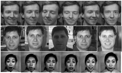
Figure 1 presents the example images of the ORL, Caltech 101, and JAFFE databases.

Figure 1. Some images from ORL (first row), Caltech 101 (second row) and JAFFE (last row).

4.2. Convergence

In this section, we empirically verify the convergence of our algorithm using different kernels, such as RBF kernel and polynomial kernel. The convergence curves of GKBNNMF-RBF and GKBNNMF-Poly on ORL dataset are given in Figure 2.

Figure 2. Convergence curve.

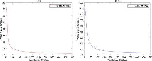
Our target matrix for decomposition is $X_{750\times 80}$, which is generated using the image data from ORL database. We set the maximum iteration number $I_{\mathrm{m}\mathrm{a}\mathrm{x}}$, feature number r, RBF kernel parameter t and polynomial kernel parameter d as $I_{\mathrm{m}\mathrm{a}\mathrm{x}}=500$, r = 80, t = 7e2 and d = 2 respectively. The curves of cost function against iteration number are plotted in Figure 2 on ORL database using GKBNNMF-RBF and GKBNNMF-poly algorithms.

At each iteration, the smaller value of the cost function is, the faster convergent speed is. It can be seen that the proposed algorithms are fastly convergent under different kernel functions.

4.3. Performance on face recognition

In our experiment, the resolution of each face image is reduced by a double $D4$ wavelet transform. Here we use the Gaussian kernel in our method (GKBNNMF) and GNMF algorithm. Five algorithms, namely, KPCA, NMF, PNMF, KNMF-RBF and GNMF-RBF are selected for comparisons. KPCA (Schökopf et al., 1998) uses the RBF kernel function $k(x,y)=\exp (-\frac{\parallel x-y{\parallel }^2}{t})$ with t = 1e2. PNMF adopts the polynomial kernel function $k(x,y)=〈x,y{〉}^d$ with d = 2. For all algorithms, the maximum number of iterations $I_{\mathrm{m}\mathrm{a}\mathrm{x}}$ is set to 300. The experiments are repeated ten times. The mean accuracy and standard deviation (std) are recorded.

4.3.1. Results on Caltech 101 database

For Caltech 101 face database, we set the feature number r to 440 during the experiment. The parameter t of RBF kernel function in KNMF-RBF, GNMF-RBF and GKBNNMF-RBF algorithms is set to $5e4$. We randomly selected $TN(TN=4,5,\dots ,8)$ images from each person as the training sample, and the remaining $(18-TN)\ast 19$ images as the testing sample. The experimental results are tabulated in Table 1 and plotted in Figures 3 and 4.

Figure 3. Recognition accuracy on Caltech 101 database.

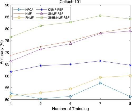
Figure 4. CMC curve comparison on Caltech 101 database.

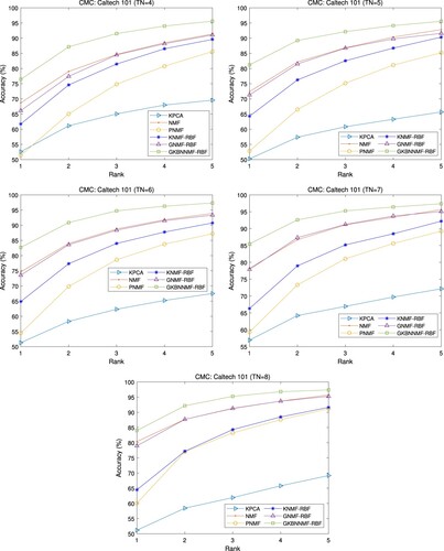
Table 1. Mean accuracy (%) and standard deviation (std) versus Training Number (TN) on Caltech 101 database.

TN	4	5	6	7	8
KPCA	52.59	50.24	51.32	56.94	51.16
(std)	(3.26)	(4.41)	(3.16)	(2.65)	(4.71)
NMF	68.68	72.39	74.61	78.23	80.37
(std)	(3.01)	(3.30)	(3.19)	(2.59)	(2.49)
PNMF	51.39	52.83	54.48	59.33	60.05
(std)	(2.81)	(3.62)	(4.27)	(3.96)	(3.62)
KNMF-RBF	61.73	64.29	64.87	66.32	64.47
(std)	(2.72)	(4.18)	(4.51)	(1.90)	(4.52)
GNMF-RBF	66.13	71.30	73.55	77.89	78.95
(std)	(2.21)	(2.67)	(3.32)	(2.13)	(2.88)
GKBNNMF-RBF	76.43	81.17	82.68	85.45	84.00
(std)	(1.00)	(1.86)	(2.03)	(2.17)	(2.70)

The mean accuracies and standard deviations (std) of the algorithms under different training samples are recorded in Table 1. We can see that the average recognition accuracy of our algorithm GKBNNMF-RBF increases from $76.43\mathrm{\%}$ with TN = 4 to $84.00\mathrm{\%}$ with TN = 8. In addition, the mean recognition accuracy of NMF (D. D. Lee & Seung, 2001), PNMF (Buciu et al., 2008), KNMF-RBF (W. S. Chen et al., 2017) and GNMF-RBF (W. S. Chen et al., 2017; Zhang & Liu, 2009) increased from $68.68\mathrm{\%}$, $51.39\mathrm{\%}$, $61.73\mathrm{\%}$ and $66.13\mathrm{\%}$ with TN = 4 to $80.37\mathrm{\%}$, $60.05\mathrm{\%}$, $64.47\mathrm{\%}$ and $78.95\mathrm{\%}$ with TN = 8. The results indicate that the proposed GKBNNMF-RBF algorithm outpeforms the other algorithms.

To show the performance of each algorithm on this database in details, we will use the cumulative match characteristic (CMC) curve with rank 1 – rank 5 accuracy for comparisons. The CMC curves are plotted in Figure 4, where the number of training samples (TN) ranges from 4 to 8. It can be seen that the CMC curves of our method are always located in the highest position, while those of KPCA are at the lowest position. This means that our GKBNNMF-RBF achieves the best performance and KPCA has the worst performance among all the compared algorithms. It also reveals that the non-negative feature is more suitable for non-negative image data in classification tasks.

4.3.2. Results on JAFFE database

For the JAFFE face database, TN (TN ranges from 3 to 7) images are randomly selected from each person as training samples, and the remaining $(20-TN)\ast 10$ images are used as testing samples. We set the feature number r of all algorithms to 450 and the parameter t of the Gaussian kernel $k(x,y)=\exp (-\frac{\parallel x-y{\parallel }^2}{t})$ in GKBNNMF-RBF, KNMF-RBF and GNMF-RBF algorithms to $5e4$. The experimental results are tabulated in Table 2, and plotted in Figures 5 and 6.

Figure 5. Recognition accuracy on JAFFE database.

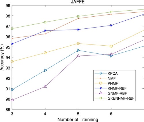
Figure 6. CMC curve comparison on JAFFE database.

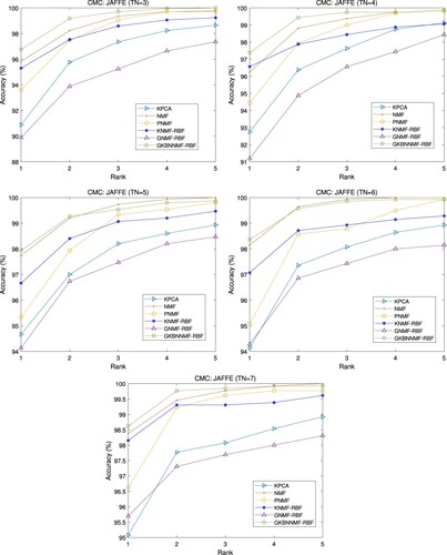
Table 2. Mean accuracy (%) and standard deviation (std) versus Training Number (TN) on JAFFE database.

TN	3	4	5	6	7
KPCA	90.88	92.75	94.67	94.14	95.08
(std)	(2.53)	(2.52)	(2.63)	(2.23)	(2.18)
NMF	95.82	96.25	97.73	98.14	98.38
(std)	(2.24)	(2.06)	(1.30)	(1.02)	(1.23)
PNMF	93.59	94.44	95.33	95.07	96.62
(std)	(4.09)	(2.27)	(2.06)	(1.04)	(2.09)
KNMF-RBF	95.29	96.56	96.67	97.07	98.15
std	(2.87)	(1.77)	(1.91)	(1.52)	(1.78)
GNMF-RBF	89.88	91.19	94.13	94.29	95.69
(std)	(4.79)	(4.26)	(3.03)	(2.33)	(2.41)
GKBNNMF-RBF	96.76	97.38	97.93	98.36	98.62
(std)	(2.44)	(1.28)	(2.05)	(1.31)	(1.49)

The average accuracy and standard deviation (std) of each algorithm under different training samples are listed in Table 2. The Rank1 recognition accuracy on the JAFFE database is plotted in Figure 5. From this figure, we observe that the average recognition rate of our proposed algorithm GKBNNMF-RBF increases from $96.76\mathrm{\%}$ with TN = 3 to $98.62\mathrm{\%}$ with TN = 7. The results on JAFFE database once again show that our algorithm has better performance than GNMF-RBF algorithm.

To further compare the performance of each algorithm, cumulative match characteristic (CMC) curves with training samples of $3,4,\dots ,7$ are drawn in Figure 6. It can be seen that when TN = 3, 4, and 7, the CMC curves of our method are at the highest position, while those of GNMF-RBF are always at the lowest position. This means that our GKBNNMF-RBF has the best performance and GNMF-RBF has the worst performance among all the compared algorithms.

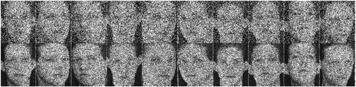
4.4. Experiments with noise

This subsection will discuss the robustness of the proposed GKBNNMF-RBF algorithm on the ORL database with Gaussian noise and speckle noise. The testing images from the ORL dataset are contaminated by zero-mean Gaussian white noise and uniformly distributed zero-mean random multiplicative noise with variance σ varying from 0.2 to 0.6, respectively. The Gaussian noised images ($\sigma =0.2$) and speckle noised images ($\sigma =0.2$) of one individual from the ORL dataset are given in Figure 7. The algorithms including KPCA, NMF, PNMF, KNMF-RBF and GNMF-RBF are adopted for comparisons. The noise experiments of the compared algorithms are run 10 times under the same conditions.

Figure 7. The Gaussian noised images (first row) and speckle noised images (second row) from ORL database $\sigma =0.2$.

4.4.1. Results with Gaussian noise on ORL database

We randomly choose three non-noised images from each person for training, and the rest seven images with Gaussian noise for testing. The feature number r of all the compared algorithms is set to 440. For the RBF kernel-based algorithms such as KNMF- RBF, GNMF-RBF and GKBNNMF-RBF, their kernel parameters t are set to $5e4$, $1e3$ and $1e3$, respectively. Their mean accuracies and standard deviations (std) are recorded in Table 3 and plotted in Figure 8. It can be seen that when the variance σ of Gaussian noise increases from 0.2 to 0.6, the accuracies of all algorithms decrease. The performance of our GKBNNMF-RBF method decreases from $85.43\mathrm{\%}$ to $61.82\mathrm{\%}$. In contrast, the performances of KPCA, NMF, PNMF, KNMF-RBF and GNMF-RBF decrease to a large extent. As can be seen from Figure 8, NMF is most sensitive to noise and its performance is significantly degraded, which indicates that the kernel-based NMF methods are more robust to noise than the linear NMF methods. It is interesting that the KNMF methods with the general kernels, namely GKBNNMF-RBF and GNMF-RBF, surpass the KNMF methods with a special kernel. GKBNNMF-RBF and GNMF-RBF have similar results when σ is less than 0.25. As σ is large than 0.25, the proposed GKBNNMF-RBF approach outperforms all the compared approaches. This means that the proposed algorithm has superior robust performance when the data are heavily contaminated.

Figure 8. Mean accuracy (%) of each algorithm when TN = 3 on ORL database with Gaussian noise.

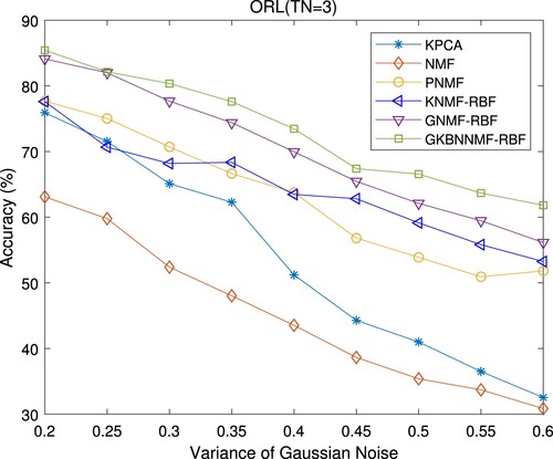
Table 3. Mean recognition rate (%) and standard deviation (std) of Gaussian noise experiment on ORL database.

σ	0.2	0.25	0.3	0.35	0.4	0.45	0.5	0.55	0.6
KPCA	75.93	71.54	65.11	62.29	51.21	44.29	41.00	36.50	32.54
(std)	(2.96)	(2.78)	(3.42)	(3.23)	(5.81)	(6.97)	(5.03)	(6.29)	(4.50)
NMF	63.11	59.79	52.39	48.04	43.54	38.64	35.39	33.71	30.86
(std)	(3.44)	(3.55)	(2.89)	(1.38)	(2.44)	(2.48)	(3.03)	(2.55)	(3.66)
PNMF	77.68	75.04	70.71	66.64	63.75	56.82	53.89	50.93	51.82
(std)	(2.77)	(2.59)	(3.04)	(3.10)	(4.27)	(4.67)	(4.94)	(5.30)	(1.69)
KNMF-RBF	77.61	70.68	68.18	68.36	63.46	62.82	59.14	55.82	53.25
(std)	(2.76)	(2.87)	(2.17)	(3.94)	(4.46)	(3.62)	(2.82)	(3.38)	(5.41)
GNMF-RBF	84.11	82.00	77.68	74.39	69.96	65.46	62.11	59.46	56.14
(std)	(2.59)	(2.80)	(1.75)	(4.01)	(4.55)	(3.79)	(4.67)	(6.87)	(2.95)
GKBNNMF-RBF	85.43	82.14	80.36	77.61	73.46	67.39	66.57	63.68	61.82
(std)	(1.84)	(1.72)	(2.95)	(3.04)	(3.52)	(2.98)	(2.93)	(5.35)	(3.64)

4.4.2. Results with speckle noise on ORL database

We randomly choose three non-noised images from each person for training, and the rest seven images with speckle noise for testing. We set the feature number r of all algorithms to 400. The parameter t of the RBF kernel in GKBNNMF-RBF, KNMF-RBF and KNMF-RBF algorithms are set to $1e3$, $5e4$ and $5e4$, respectively. The average accuracies and standard deviations (std) of all the compared methods are tabulated in Table 4 and plotted in Figures 9. It indicates that the performances of all the compared algorithms decrease as the intensity of the speckle noise increases. We can see that when the variance of speckle-noise raises from 0.2 to 0.6, the accuracy of our GKBNNMF-RBF algorithm decreases from 91.82 to 89.68. The results show that the proposed GKBNNMF-RBF approach achieves the best performance under different levels of speckle noises. GNMF-RBF is the second-best algorithm among the compared algorithms, while NMF is most sensitive to speckle noise and its performance is the most severely degraded as the speckle noise is raised. Especially, with the variations of variance in speckle noise, our GKBNNMF-RBF method has the smallest changes in recognition accuracy. This means that the proposed algorithm has good robustness to speckle noise.

Figure 9. Mean accuracy (%) on ORL database with TN = 3 under different speckle noises.

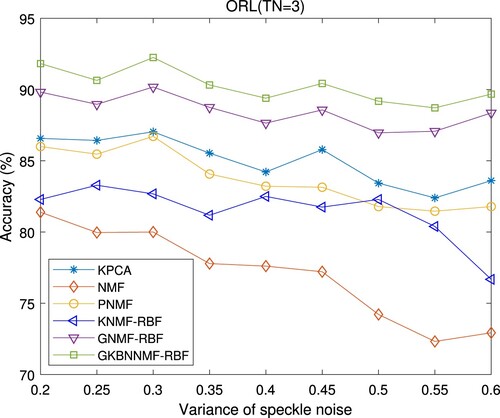
Table 4. Mean recognition rate (%) and standard deviation (std) of speckle noise experiment on ORL database.

σ	0.2	0.25	0.3	0.35	0.4	0.45	0.5	0.55	0.6
KPCA	86.57	86.43	87.04	85.54	84.21	85.79	83.43	82.39	83.61
(std)	(1.73)	(2.23)	(2.25)	(2.31)	(3.14)	(1.63)	(2.14)	(2.46)	(3.66)
NMF	81.39	79.96	80.00	77.79	77.61	77.21	74.21	72.32	72.93
(std)	(2.54)	(3.35)	(1.67)	(2.26)	(1.91)	(1.73)	(2.06)	(1.96)	(2.07)
PNMF	86.00	85.46	86.71	84.07	83.21	83.14	81.79	81.46	81.79
(std)	(2.63)	(2.53)	(2.12)	(2.68)	(2.56)	(2.87)	(2.95)	(2.27)	(2.45)
KNMF-RBF	82.29	83.29	82.68	81.18	82.50	81.75	82.29	80.39	76.68
(std)	(1.98)	(2.11)	(2.48)	(2.27)	(2.91)	(3.01)	(2.38)	(2.59)	(1.86)
GNMF-RBF	89.82	88.96	90.18	88.75	87.64	88.57	86.96	87.07	88.36
(std)	(2.40)	(1.75)	(1.83)	(1.68)	(2.84)	(2.40)	(2.33)	(2.69)	(2.91)
GKBNNMF-RBF	91.82	90.64	92.25	90.32	89.39	90.43	89.18	88.71	89.68
(std)	(2.52)	(1.48)	(1.32)	(2.13)	(3.38)	(1.80)	(2.64)	(3.08)	(2.80)

4.5. Results on JAFFE database

For the JAFFE database, we compare GKBNNMF algorithms using different kernel functions to GNMF, PNMF and FPKNMF algorithms. We set the feature number r of each algorithm to 450, and the parameter t of the RBF kernel function of GKBNNMF-RBF and GNMF-RBF algorithm to $5e4$ and $5e5$ respectively. The parameter of polynomial kernel is set to 6, and that of fractional inner product kernel is set to 0.5.

Table 5 lists the average accuracy and standard deviation of each algorithm under different training samples. The $Rank1$ recognition rates on the JAFFE database are plotted in Figure 10. The CMC curves with training samples of $3,4,\dots ,7$ are also plotted in Figure 11. We observe that GKBNNMF-RBF has the best performance. The performance of FPKNMF is the second best. The results also show that GKBNNMF outperforms GNMF when they use the same type of kernel.

Figure 10. Recognition accuracy on JAFFE database.

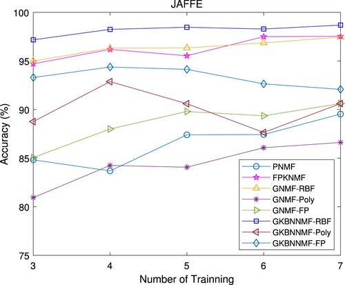
Figure 11. CMC curve comparison on JAFFE database.

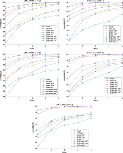
Table 5. Mean accuracy (%) versus Training Number (TN) on JAFFE database.

TN	3	4	5	6	7
PNMF	84.82	83.69	87.40	87.43	89.54
(std)	(3.61)	(4.58)	(4.85)	(2.66)	(2.59)
FPKNMF	94.71	96.19	95.53	97.50	97.54
(std)	(1.84)	(2.13)	(1.81)	(1.27)	(1.88)
GNMF-RBF	95.00	96.31	96.33	96.86	97.46
(std)	(2.31)	(2.15)	(1.99)	(1.59)	(1.58)
GNMF-Poly	80.94	84.25	84.07	86.07	86.62
(std)	(5.48)	(4.02)	(3.72)	(4.07)	(4.26)
GNMF-FP	85.06	88.00	89.80	89.36	90.62
(std)	(5.25)	(5.19)	(3.49)	(3.93)	(3.59)
GKBNNMF-RBF	97.18	98.25	98.47	98.29	98.69
(std)	(2.25)	(1.01)	(1.78)	(0.37)	(1.26)
GKBNNMF-Poly	88.76	92.88	90.60	87.64	90.62
(std)	(4.62)	(3.43)	(3.01)	(6.05)	(2.92)
GKBNNMF-FP	93.29	94.38	94.13	92.64	92.08
(std)	(3.65)	(2.41)	(1.66)	(3.28)	(3.94)

5. Conclusion

It is known that the existing KNMF methods mainly encounter problems including inaccurate pre-image learning and non-universal use of kernels. This paper focuses on these problems and proposes a general kernel-based non-negative matrix factorisation (GKBNNMF) approach, which can overcome the drawbacks of existing KNMF methods. We establish the GKBNNMF model using the symmetric NMF technique to ensure the non-negativity of the decomposition. The proposed GKBNNMF algorithm is shown to be convergent by theoretical analysis and empirical validation. The experiments on face recognition have demonstrated the effectiveness of our approach.

There are several challenges that need to be met in future study. First, the performance of the algorithm is sensitive to the setting of the hyperparameters including the characteristic number r and the kernel parameters. Currently, we set these hyperparameters manually. The initialisation matrices are also crucial to the performance. The cross-validation technique and some initialisation methods of NMF (Atif et al., 2019) could be considered to find good values of these hyperparameters.

Second, faster implementations of our method for large-scale data are also important for future research. The low-rank approximation of kernel method (Fine & Scheinberg, 2002) could be considered to speed up the algorithm. Alternatively, we can use the block technique (Pan et al., 2011) to reduce the size of the matrix, which may also reduce the computational complexity of the algorithm.

Finally, our method relies on the non-negativity of the kernel matrix, which can be ensured for the commonly used kernel functions. However, if the non-negativity of the kernel matrix is not satisfied, other factorisation instead of symmetric NMF should be used.

Disclosure statement

No potential conflict of interest was reported by the author(s).

Additional information

Funding

This work was partially supported by the Natural Science Foundation of Shenzhen (20200815000520001) and the Interdisciplinary Innovation Team of Shenzhen University.

References

- Akbarizadeh, G. (2012). A new statistical-based kurtosis wavelet energy feature for texture recognition of SAR images. IEEE Transactions on Geoscience and Remote Sensing, 50(11), 4358–4368. https://doi.org/10.1109/TGRS.2012.2194787
- Atif, S. M., Qazi, S., & Gillis, N. (2019). Improved SVD-based initialization for nonnegative matrix factorization using low-rank correction. Pattern Recognition Letters, 122, 53–59. https://doi.org/10.1016/j.patrec.2019.02.018.
- Belhumeur, P. N., Hespanha, J. P., & Kriegman, D. J. (1997). Eigenfaces vs. fisherfaces: recognition using class specific linear projection. IEEE Transactions on Pattern Analysis and Machine Intelligence, 19(7), 711–720. https://doi.org/10.1109/34.598228
- Buciu, I., Nikolaidis, N., & Pitas, I. (2008). Nonnegative matrix factorization in polynomial feature space. IEEE Transactions on Neural Networks, 19(6), 1090–1100. https://doi.org/10.1109/TNN.2008.2000162
- Chen, J. H., Qin, J. H., Xiang, X. Y., & Tan, Y. (2020). A new encrypted image retrieval method based on feature fusion in cloud computing. International Journal of Computational Science and Engineering, 22(1), 114–123. https://doi.org/10.1504/IJCSE.2020.107261
- Chen, W. S., Huang, X. K., Pan, B., Wang, Q., & Wang, B. H. (2017). Kernel nonnegative matrix factorization with RBF kernel function for face recognition. In International conference on machine learning & cybernetics (ICMLC) (pp. 285–289). Editors: P. Shi etc., Publisher: Institute of Electrical and Electronics Engineers Inc., United States.
- Chen, W. S., Liu, J. M., Pan, B., & Chen, B. (2019). Face recognition using nonnegative matrix factorization with fractional power inner product kernel. Neurocomputing, 348(10), 40–53. https://doi.org/10.1016/j.neucom.2018.06.083
- Chen, W. S., Qian, H. H., Pan, B., & Chen, B. (2020). Kernel non-negative matrix factorization using self-constructed cosine kernel. In 16th international conference on computational intelligence and security (CIS) (pp. 186–190). Editors: Y. P. Wang etc., Publisher: Elsevier B. V.
- Cheng, J., Liu, Q. S., Lu, H. Q., & Chen, Y. W. (2005). Supervised kernel locality preserving projections for face recognition. Neurocomputing, 67(7), 443–449. https://doi.org/10.1016/j.neucom.2004.08.006
- Davari, N., Akbarizadeh, G., & Mashhour, E. (2020). Intelligent diagnosis of incipient fault in power distribution lines based on corona detection in UV-visible videos. IEEE Transactions on Power Delivery. https://doi.org/10.1109/TPWRD.2020.3046161.
- Deng, C., He, X., Han, J., & Huang, T. S. (2011). Graph regularized nonnegative matrix factorization for data representation. IEEE Transactions on Pattern Analysis and Machine Intelligence, 33(8), 1548–1560. https://doi.org/10.1109/TPAMI.2010.231
- Eggert, J., & Korner, E. (2004). Sparse coding and NMF. In 2004 IEEE international joint conference on neural networks (Vol. 4, pp. 2529–2533). Editors: Joos Vandewalle etc., Publisher: IEEE.
- Fine, S., & Scheinberg, K. (2002). Efficient SVM training using low-rank kernel representations. Journal of Machine Learning Research, 2(2), 243–264. https://doi.org/10.1162/15324430260185619.
- Guillamet, D., Schiele, B., & Vitria, J. (2002). Analyzing non-negative matrix factorization for image classification. In 16th international conference on pattern recognition (pp. 116–119). Editors: R. Kasturi etc., Publisher: IEEE.
- Hancer, E. (2019). Fuzzy kernel feature selection with multi-objective differential evolution algorithm. Connection Science, 31(4), 323–341. https://doi.org/10.1080/09540091.2019.1639624
- He, C. B., Zhang, Q., Tang, Y., Liu, S. Y., & Liu, H. (2019). Network embedding using semi-supervised kernel nonnegative matrix factorization. IEEE Access, 7, 92732–92744. https://doi.org/10.1109/Access.6287639
- He, X. (2003). Locality preserving projections. In Advances in neural information processing systems (pp. 186–197). Editors: S. Thrun etc., Publisher: MIT Press.
- He, Z., Xie, S., Zdunek, R., Zhou, G., & Cichocki, A. (2011). Symmetric nonnegative matrix factorization: algorithms and applications to probabilistic clustering. IEEE Transactions on Neural Networks, 22(12), 2117–2131. https://doi.org/10.1109/TNN.2011.2172457
- Hoyer, P. O. (2004). Nonnegative matrix factorization with sparseness constraints. Journal of Machine Learning Research, 5(9), 1457–1469. DOI:10.1016/j.neucom.2011.09.024.
- Lee, D. D., & Seung, H. S. (1999). Learning the parts of objects by non-negative matrix factorization. Nature, 401(667), 788–791. https://doi.org/10.1038/44565
- Lee, D. D., & Seung, H. S. (2001). Algorithms for non-negative matrix factorization. In Advances in neural information processing systems (pp. 556–562). Editors: T. Dietterich etc., Publisher: MIT Press.
- Lee, H., Yoo, J., & Choi, S. (2010). Semi-supervised nonnegative matrix factorization. IEEE Signal Processing Letters, 17(1), 4–7. https://doi.org/10.1109/LSP.2009.2027163
- Li, S. Z., Hou, X. W., Zhang, H. J., & Cheng, Q. S. (2001). Learning spatially localized, parts-based representation. In IEEE conference on computer vision and pattern recognition (CVPR) (pp. 207–212). Editors: Anne Jacobs and Thomas Baldwin. Publisher: IEEE.
- Lin, C. (2014). Projected gradient methods for nonnegative matrix factorization. Neural Computation, 19(10), 2756–2779. https://doi.org/10.1162/neco.2007.19.10.2756
- Liu, W. X., & Zheng, N. N. (2004). Non-negative matrix factorization based methods for object recognition. Pattern Recognition Letters, 25(8), 893–897. https://doi.org/10.1016/j.patrec.2004.02.002
- Liu, X. Z., & Ruan, H. Y. (2019). Kernel-based tensor discriminant analysis with fuzzy fusion for face recognition. International Journal of Computational Science and Engineering, 19(2), 293–300. https://doi.org/10.1504/IJCSE.2019.100233
- Martinez, D., & Bray, A. (2003). Nonlinear blind source separation using kernels. IEEE Transactions on Neural Networks, 14(1), 228–235. https://doi.org/10.1109/TNN.2002.806624
- Nagra, A. A., Han, F., Ling, Q. H., Abubaker, M., Ahmad, F., Mehta, S., & Apasiba, A. T. (2020). Hybrid self-inertia weight adaptive particle swarm optimisation with local search using C4.5 decision tree classifier for feature selection problems. Connection Science, 32(1), 16–36. https://doi.org/10.1080/09540091.2019.1609419
- Novak, M., & Mammone, R. (2001). Use of nonnegative matrix factorization for language model adaptation in a lecture transcription task. In Proceedings of IEEE international conference on acoustics, speech, and signal processing (pp. 541–544). Editor: V. John Mathews. Publisher: IEEE.
- Paatero, P., & Tapper, U. (1994). Positive matrix factorization: a non-negative factor model with optimal utilization of error estimates of data values. Environmetrics, 5(2), 111–126. https://doi.org/10.1002/(ISSN)1099-095X
- Pan, B., Lai, J., & Chen, W. S. (2011). Nonlinear nonnegative matrix factorization based on Mercer kernel construction. Pattern Recognition, 44(10–11), 2800–2810. https://doi.org/10.1016/j.patcog.2011.03.023
- Pekalska, E., & Haasdonk, B. (2009). Kernel discriminant analysis for positive definite and indefinite kernels. IEEE Transactions on Pattern Analysis and Machine Intelligence, 31(6), 1017–1032. https://doi.org/10.1109/TPAMI.2008.290
- Plumbley, M. D., Abdallah, S. A., Bello, J. P., Davies, M. E., Monti, G., & Sandler, M. B. (2002). Automatic music transcription and audio source separation. Cybernetics and Systems, 33(6), 603–627. https://doi.org/10.1080/01969720290040777
- Qian, J., Zhao, R., Wei, J., Luo, X., & Xue, Y. (2020). Feature extraction method based on point pair hierarchical clustering. Connection Science, 32(3), 223–238. https://doi.org/10.1080/09540091.2019.1674246
- Schökopf, B., Smola, A., & Müller, K. R. (1998). Nonlinear component analysis as a kernel eigenvalue problem. Neural Computation, 10(5), 1299–1319. https://doi.org/10.1162/089976698300017467
- Shi, M., Yi, Q. M., & Lv, J. (2012). Symmetric nonnegative matrix factorization with beta-divergences. IEEE Signal Processing Letters, 19(8), 539–542. https://doi.org/10.1109/LSP.2012.2205238
- Tirandaz, Z., & Akbarizadeh, G. (2015). A two-phase algorithm based on kurtosis curvelet energy and unsupervised spectral regression for segmentation of SAR images. IEEE Journal of Selected Topics in Applied Earth Observations and Remote Sensing, 9(3), 1244–1264. https://doi.org/10.1109/JSTARS.4609443
- Tirandaz, Z., Akbarizadeh, G., & Kaabi, H. (2020). PolSAR image segmentation based on feature extraction and data compression using weighted neighborhood filter bank and hidden Markov random field-expectation maximization. Measurement, 153(2), 107432. https://doi.org/10.1016/j.measurement.2019.107432
- Too, E. C., Li, Y., Gadosey, P. K., Njuki, S., & Essaf, F. (2020). Performance analysis of nonlinear activation function in convolution neural network for image classification. International Journal of Computational Science and Engineering, 21(4), 522–535. https://doi.org/10.1504/IJCSE.2020.106866
- Turk, M. A., & Pentland, A. P. (1991). Face recognition using eigenfaces. In IEEE conference on computer vision and pattern recognition (CVPR) (pp. 586–591). Editor: Alan H. Barr. Publisher: IEEE.
- Xu, W., Liu, X., & Gong, Y. H. (2003). Document clustering based on non-negative matrix factorization. In Proceedings of SIGIR (pp. 267–273). Editors: Charles Clarke etc., Publisher: Association for Computing Machinery, New York, NY, United States. https://doi.org/10.1145/860435.860485
- Yi, S. Y., Lai, Z. H., He, Z. Y., Cheung, Y. M., & Liu, Y. (2017). Joint sparse principal component analysis. Pattern Recognition, 61(7), 524–536. https://doi.org/10.1016/j.patcog.2016.08.025
- Yu, H., & Yang, J. (2001). A direct LDA algorithm for high-dimensional data: with application to face recognition. Pattern Recognition, 34(10), 2067–2070. https://doi.org/10.1016/S0031-3203(00)00162-X
- Zafeiriou, S., & Petrou, M. (2010). Nonlinear non-negative component analysis algorithms. IEEE Transactions on Image Processing, 19(4), 1050–1066. https://doi.org/10.1109/TIP.2009.2038816
- Zafeiriou, S., Tefas, A., Buciu, I., & Pitas, I. (2006). Exploiting discriminant information in nonnegative matrix factorization with application to frontal face verification. IEEE Transactions on Neural Networks, 17(3), 683–695. https://doi.org/10.1109/TNN.2006.873291
- Zalpour, M., Akbarizadeh, G., & Alaei-Sheini, N. (2020). A new approach for oil tank detection using deep learning features with control false alarm rate in high-resolution satellite imagery. International Journal of Remote Sensing, 41(6), 2239–2262. https://doi.org/10.1080/01431161.2019.1685720
- Zhang, D. Q., & Liu, W. Q. (2009). An efficient nonnegative matrix factorization approach in flexible kernel space. In Proceedings of the twenty-first international joint conference on artificial intelligence (pp 1345–1350). Publisher: International Joint Conferences on Artificial Intelligence.
- Zhou, Y., & Cheung, Y. M. (2021). Bayesian low-tubal-rank robust tensor factorization with multi-rank determination. IEEE Transactions on Pattern Analysis and Machine Intelligence, 43(1), 62–76. https://doi.org/10.1109/TPAMI.34
- Zhu, F., Honeine, P., & Kallas, M. (2014). Kernel nonnegative matrix factorization without the curse of the pre-image: application to unmixing hyperspectral images. In IEEE international workshop on machine learning for signal processing (pp. 1–6). Editors: Mamadou Mboup etc., Publisher: IEEE.