Automatic traffic modelling for creating digital twins to facilitate autonomous vehicle development

Abstract

A digital twin is often adopted in computer simulations to expedite autonomous vehicle developments by using the simulated 3D environment that reflects a physical environment. In particular, traffic simulations are a crucial part of training the driving logic before the field test of an autonomous vehicle is performed on specific regions to adapt to the region-specific, dynamic traffic conditions. Currently, the traffic conditions are either synthesised by tools (e.g. using mathematical models) or created manually (using domain knowledge), which cannot reflect the realistic, region-specific conditions or will require extensive labour works. In this article, we propose an automatic methodology to model the real-world traffic conditions captured by the sensor data and to reproduce the modeled traffic in the digital twin. We have built the tools based on the methodology and use the KITTI dataset to validate the effectiveness of the tools. To recreate the region-specific traffic, we present the results of capturing, modelling, and recreating the two-wheeler traffic condition on the Southeast Asia road. Our experimental results show that the proposed method facilitates the simulation of real-world, Southeast Asia-specific traffic conditions by removing the needs of the synthesised traffic and the labour hours.

Keywords:

• Traff modelling
• Digital twins
• Autonomous vehicle
• 3D simulations
• Modelling moving tracks

1. Introduction

Simulations are widely adopted to facilitate the development of autonomous vehicle system designs. Autonomous vehicle simulation recreates a physical environment by feeding the environmental sensor data to the autonomous driving system, so that the driving software can perceive, make a decision, plan a route, and issue control command, as if it is in the physical environment. The simulation provides a controlled and safe environment for the development and test of autonomous driving systems. It is a common way to develop the prototype software (e.g. for a novel navigation algorithm) within the simulated environment first before the software could be deployed to the physical vehicle running in the real-world environment.

A digital twin is the digital version of a physical object or system; in the context of autonomous vehicle simulations, the key to the success of simulation-based system development is the level of the details for the digital twin recreated by the simulators. The digital twin with high-level details of the physical counterpart provides a perfect environment for autonomous vehicle development since the perceived sensor data within the digital twin are very close to those obtained from the real-world counterpart.

Creating the digital replica of a physical environment is an important but time-consuming and labour-intensive job. The digital twin of a traffic scene usually consists of both the hardware and the software parts. The digital hardware infrastructure refers to those objects that are stationary in fixed locations (e.g. traffic signs, road layout, lanes of a road, street lights, and surrounding buildings), where the objects are often represented by the models of 3D computer graphics and it usually requires intensive manual works to construct the 3D models for the physical counterparts. With the hardware part, the autonomous vehicles can be trained in the simulations for how to drive properly, e.g. knowing when to move/stop by reading the traffic signals, following a car lane instead of driving in-between two lanes by recognising the lane marks, and facilitating the vehicle positioning by referencing the surrounding buildings (e.g. by using LiDAR data). On the other hand, the software part is more like the traffic conditions observed by the autonomous vehicles at different time points (e.g. numbers of vehicles/motorcycles/pedestrians on the road and their moving paths, weather conditions, and daylight). Through the simulation configurations, the dynamic traffic conditions can be imitated in the digital world, which helps train the vehicles to drive safely by anticipating the traffic and coping with it (e.g. knowing how to drive smoothly and safely when entering the area crowed with motorcycles under heavy rain). Combining the two parts together, the digital twin is capable of recreating a specific traffic condition for accumulating the driving miles for the autonomous vehicles before testing in the physical world.

Some tools have been made to help accelerate the constructions of 3D objects for the hardware part (e.g. map annotation tools from SVL simulator). Unfortunately, on the other hand, the software part regarding the traffic conditions is more dynamic and is difficult to be recreated for the certain traffic scene. For example, people from different regions/countries would have distinctive riding/driving behaviours resulting from specific traffic regulations, which requires the time to observe and model those behaviours in the digital world. According to the best of our knowledge, while there are tools developed for modelling a large-scale traffic and performing the simulation (Lee & Wong, 2016a; Pell et al., 2017; PTV Group, 2021; Wismans et al., 2014; Xu et al., 2021), we are not aware of the research work that helps replicate the real-world traffic and recreate the replicated (modeled) traffic in the simulated 3D environment automatically.

In this article, we present the automatic traffic modelling by capturing the sensor data of real-world traffic and replicating the digital twin version of the traffic condition surrounding the autonomous vehicle, so that the autonomous vehicle is able to be tested with the captured realistic traffic within the simulated environment. The automatic traffic modelling removes the need for manual works to observe, model, and design the traffic with different types of objects (e.g, pedestrians, motorcycles, and cars). The modeled traffic reflects the real-world conditions (i.e. moving tracks, speeds, and postures), which help developers acquire more realistic data for training the autonomous driving software off-line. For example, in the regions of Southeast Asia, two-wheelers are popular on the roads, and they can often exhibit distinct riding styles different from the four-wheelers, e.g. motorcycles driving between two lanes, and bicycles riding in the opposite direction toward the vehicle. In such a case, an automatic traffic modelling and replicating method is critical to capture the real-world traffic so as to train the autonomous driving software in a more realistic environment, rather than the traffic synthesised manually that requires extensive labour works and cannot effectively reflect the region-specific real-world traffic conditions. Moreover, our work only uses LiDAR data as a tracking method to validate the feasibility of automatic traffic modelling in simulation, which implies the different sensor algorithms could further model the more sophisticated traffic.

We have developed the tools to automate the traffic modelling and recreating. Our experimental results show that the proposed method can effectively recreate the two-wheeler traffic and help the development of autonomous driving algorithms. With the proposed method, the makers of autonomous vehicles are able to train the driving logic to adapt to the region-specific traffic within a safe and controlled environment before the vehicles are sold to different regional markets. The contributions of this work are summarised as follows.

1. We propose the automatic traffic modelling method to model the real-world traffic and to recreate the modeled traffic in the simulated 3D environment. Furthermore, the proposed method automates the modelling and recreating of the region-specific traffic and thus, helps facilitate the training of the autonomous vehicles via 3D simulations. To the best of our knowledge, we are not aware of any other work that focuses on automatically capturing and recreating the realistic traffic for the 3D simulations.

2. We develop the software tool for the automatic traffic modelling, and the functionality is validated by the KITTI dataset. In particular, the developed tool accepts the LiDAR point cloud data from the KITTI dataset, recognises the moving objects and their properties (e.g.moving tracks), and reproduces the moving trajectories of the recognised objects in the 3D simulations.

3. We demonstrate the capability of our proposed method with several traffic scenarios which are commonly seen in the regions of Southeast Asia. Especially, we record the traffic scenario of the motorcycle overtaking in the physical environment and reproduce the modeled traffic with the 3D simulation. The result shows that our proposed method is effective and is capable of reproducing the realistic traffic in the simulated environment.

The rest of this paper is organised as follows. Section 2 provides the information of 3D simulation tools and autonomous driving software. Section 3 presents the workflow of the proposed traffic modelling work. The preliminary results of our proposed method are presented in Section 4. Section 5 concludes this work.

2. Background

We first brief the simulation schemes for the autonomous vehicle development. We then present the related work of the 3D simulation tools and the software for autonomous vehicles.

2.1. Computer simulations for autonomous vehicle development

As for autonomous vehicle system development, the simulations can be categorised into two simulation schemes based on the participants (i.e.software) involved in the simulation. The first is the co-simulation scheme, where the 3D simulation provides a digital version of the target scene from the physical world and the simulated vehicle obtains the sensor data generated by the 3D simulator to react and drive in the digital world. Figure 1 illustrates its setup, where the 3D simulation is run on one computer (PC1) and the software for controlling the emulated autonomous vehicle within the 3D environment is run on the other computer (PC2). These two computers are linked by Ethernet to exchange messages. The setup is referred to as the co-simulation scheme as the two pieces of software are run concurrently and collaboratively for the autonomous vehicle simulation.

Figure 1. The organisation of the autonomous vehicle simulation with two computers, where the 3D environment simulation is done in PC1 and the controlling of the simulated autonomous vehicle is done in PC2.

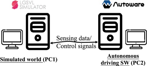
While it is possible to do the co-simulation in a single, powerful server, it makes it hard to project the delivered performance of the autonomous driving system since the 3D simulation tends to demand for computing powers and performing the co-simulation within a single computer degrades the delivered performance of both the 3D simulation and the autonomous driving software. Therefore, it is a common way to use the setup shown in Figure 1 for the autonomous vehicle simulation; based on our experiences, the Gigabyte Ethernet is sufficient for transmitting the sensor data with low-resolution camera stream data and LiDAR point cloud. If a larger size of sensor data is to be transferred for the autonomous vehicle simulation, the network bandwidth should be estimated carefully to make sure that the data transferring rate is not affected.

It is interesting to note that the setup has an obvious advantage; that is, if the data rate in the co-simulation environment matches those on the physical environment, the measured performance on PC2 reflects the observed performance on the physical counterpart of autonomous vehicle. In other words, it is possible to use the performance measured on PC2 as an indicator for the delivered performance on the physical hardware (vehicle). Hence, the setup is good for both software development and performance projections for the autonomous vehicle development, and the co-simulation scheme is adopted by this work to facilitate the system development. Although the co-simulation scheme can help developers observe the real-time response of algorithms and provide flexibility of scenario adjustment, it comes with higher costs (i.e. two high-end servers), and the performance of the simulation is limited by the network bandwidth.

The second is the standalone scheme, where the autonomous driving software is running on its own driven by the pre-recorded sensor data (without the 3D simulator feeding the sensor data at runtime). The validation of the algorithms is limited as sensor data is pre-recorded on a certain route (either in the physical or simulated environment), e.g.the inability of the feedback control and the monotonous scenarios. In addition, depending on the number of sensor data to be collected, the storage size of the pre-recorded sensor data grows linearly, which implies the length of the time and the number of the sensor data to be recorded are limited.

Compared with training an autonomous driving vehicle in the physical environment, the limitation of the co-simulation scheme is that there may be some discrepancies between the real and virtual environments (e.g. the out-dated 3D models and the unrealistic traffic in 3D simulations), meaning that the validation process should be done in the real environment to ensure the correctness/efficiency of the autonomous driving software after the prototyping and testing of the software are done in the virtual environment. Our developed traffic modelling/recreating method tackles the problem by minimising the discrepancy between the real world and the simulated traffic. In addition, while the standalone scheme recording the data in the physical environment avoids the mismatching problem, it limits the scope of the software testing since the driving software receives the pre-recorded data with a fixed number of sensor data on the designated route. Furthermore, it cannot provide the opportunity for the autonomous vehicle to interact with the surrounding environments because the recorded data are replayed to the autonomous driving software, whose feedback control cannot alter the input data. Given that each scheme has its own limitations, it is important to choose the scheme wisely based on the need during the software development process.

2.2. 3D simulation tools

Conventional traffic simulation tools focus on estimating the status for larger-scale traffic flows, which is good for traffic management in cities. For instance, the tools can be used to evaluate the performance impact of a certain arrangement on the city traffic by estimating the traffic speed with a specific traffic signal management plan under a given traffic flow. PTV Vissim (PTV Group, 2021) is a remarkable example, and it provides multiple simulation models for imitating traffic in cities. Particularly, PTV Vissim has the microscopic simulation model, which allows the simulation of each entity (e.g. car, bus, motorcycle) and observing their interactions by applying different models for a large scale traffic on top of Vissim (Lee & Wong, 2016a; Pell et al., 2017; Rodrigues et al., 2021; Wismans et al., 2014; Yao et al., 2020). Nevertheless, these tools are not sufficient for training the autonomous driving software since they cannot establish a digital twin offering a higher level of details for the simulated objects during the simulation. Instead, they are designed for modelling the larger scale traffic, which renders these tools improper for training the driving logic of an autonomous vehicle.

More recently, the 3D simulations have been developed to create the digital environments for autonomous vehicle development. The tools include Cognata (Cognata, 2020), Nvidia Drive Constellation (Nvidia, 2020), and rFpro (rFpro, 2020). In addition to the commercial-grade simulators, the open-source simulation tools are also available, e.g. CARLA (CARLA, 2020) and SVL Simulator (Rong et al., 2020), and they can be downloaded freely for research purposes. The 3D simulation tools are different from the conventional tools in that they focus on mimicking the environment (i.e.digital twin) as if it is in the physical environment. Specifically, the environment sensed by an autonomous vehicle in the 3D simulation would be close to that perceived in the physical world (e.g. the generated LiDAR data in the virtual and real environments are alike). Thus, the full-scale autonomous driving software can be exercised in 3D simulations to accumulate the driving experiences, which is not supported by the conventional tools.

Thanks to the benefits brought by 3D simulations, such as rapid deployment, risk avoidance, and budget reduction, many works have been proposed to develop the algorithms within the virtualised environments. Wang et al. (2021) introduce a digital twin simulation architecture based on the Unity 3D engines, which requires human control to follow the preceding vehicle within the Unity environment. Liu et al. (2020) integrate the camera image and the pre-built cloud digital twin information to improve the visual guidance system. OpenCDA (Xu et al., 2021) leverages a co-simulation platform with simulators, a full-stack cooperative driving system, and a scenario manager to help developers deploy the cooperative driving automation system. The above works show that the simulated systems do improve the process of the algorithm development significantly. Nevertheless, they need a significant amount of labour works to design and arrange a realistic traffic scenario within the simulated environment for validating/testing the driving algorithms.

In this work, we use the SVL simulator to enable the full-stack autonomous driving software execution to better understand the functional and performance-wise behaviours to facilitate the autonomous system design process. The SVL simulator is equipped with various types of sensors that are commonly seen in autonomous vehicles, such as GPS, LiDAR, Camera, Radar, and Ultrasonic. These sensor data mimic the data to be captured in the physical environment (sensed by autonomous vehicles) and can drive the execution of the full software stack of autonomous driving software as if in the physical environment. With the 3D simulators, such as the SVL simulator, the desired physical environments can be constructed in the simulated counterparts to facilitate the training of the knowledge of the autonomous driving software in the controlled environments. In addition, it allows its users to control the weather, the map, and the non-player characters (NPC) to recreate the specific traffic scene for testing. The simulator also incorporates with the popular game engine, Unity, to handle the 3D objects, scenes, and the mimicking of 3D effects for the objects. Nevertheless, currently, the traffic in the simulated environment should be created manually by the developers, which is a time-consuming job and may not reflect the actual traffic conditions seen in the real world. This work is proposed to address the problems and our approach is able to expedite the development process of the autonomous driving software. More about the efforts to be made for modelling the real-world traffic and replicating the traffic in the simulated world are presented in Section 3.

2.3. Autonomous driving software

Autonomous driving software is the central control of an autonomous vehicle, and it receives the sensor data and reacts based on the perceived information. The autonomous driving software is considered as a platform that consolidates different algorithms to facilitate the self-driving researches, such as Zhao et al. (2021), Das and Chand (2021), Jiang et al. (2021), and Zhang et al. (2021). In addition to those proprietary solutions, Apollo (Baidu, 2020) and Autoware (Kato et al., 2015) are the open-source alternatives, both of which are highly integrated with the SVL simulator for autonomous vehicle simulations. In this work, we use the Robot Operating System (ROS) based driving software, Autoware, to facilitate the development of traffic modelling; further information is detailed in Section 4; note that ROS is a software framework to create robotic applications. In the real world, Autoware is running within the physical vehicle. On the contrary, in the simulated environment, Autoware can be run in either the co-simulation scheme or the standalone scheme.

3. Traffic modeling for digital twins creation

To build the digital twin that recreates an observed traffic condition on a given 3D map for the autonomous vehicle simulation, in this section, we first describe the methods we used to capture the traffic condition, and then we highlight the key points that are required to import the captured traffic into the 3D simulation tool.

3.1. Traffic condition modeling

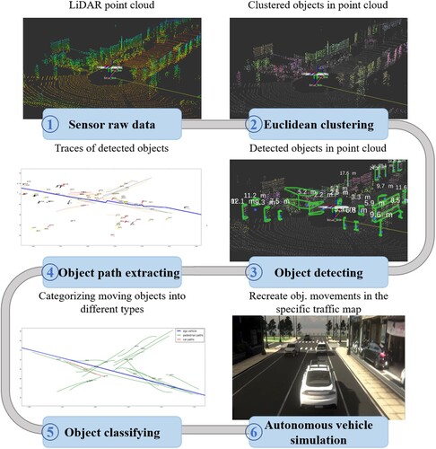
Our proposed solution helps rapidly model the desired traffic and reproduce the scenario in the simulation environment. The workflow of our proposed method is illustrated in Figure 2. The modelling process consists of six steps, and it starts from obtaining the LiDAR point cloud data as the first step to characterise the physical environment. The second step is responsible for grouping the nearby data points in the point could and the clustered data points are the candidates for the object detection in the third step, which further detects and labels the objects from the point cloud clusters and the properties of the detected objects (e.g. orientation) are derived in this step. In the object path extracting step, the detected objects are further analysed under the moving time windows to extract their continuous movements (i.e. object trajectories), where the stationary and moving objects can be identified in this step. In the fifth step, the types of the moving objects are classified (e.g. cars and motorcycles) and the stationary objects (e.g. parked cars) are filtered out in this step. The final step maps the captured object trajectories onto the selected map for the 3D simulation. The detail of each step is described as follows.

Figure 2. The workflow of our object path extractor, where it takes LiDAR sensing data as input and generates the travel paths of the detected objects for SVL simulator.

3.1.1. Sensor data

While video data can be served for similar purposes, processing the video streaming data often requires a more powerful computer to calculate the desired data, which is explained in the following paragraphs. In this work, we track objects with the measurements from a LiDAR sensor mounted on top of an ego vehicle, and a point cloud is the measured data reported by the sensor. A point cloud is usually recorded and replayed to autonomous vehicle software as one of the input sensor data for the autonomous vehicle simulation. For instance, Autoware can take the point cloud data stored in the rosbag format to drive the autonomous vehicle simulation, using the standalone scheme as mentioned in Section 2.2. A point cloud data is often comprised of three channels (of x-, y-, and z-coordinates) and records the states of the surrounding environment in a specific time period.

3.1.2. Euclidean clustering

We adopt the distance-based cluster algorithm to identify the objects within a given point cloud data, where the Euclidean distance is used to group the nearby data points. Specifically, to group all the points for a cluster, some point cloud data are used as seed points for growing a region. Each of the grouped clusters is labelled with a distinctive cluster identifier, which is useful for visualisation (of debug purpose) and for tracking in the later stages.

3.1.3. Object detecting

The detection of objects in point clouds is further decomposed into two procedures: detecting desired objects and calculating the moving tracks of the detected objects.

• The bounding box-based detecting algorithm is adopted to further detect the objects clustered in the previous step, where the L-shape bounding box algorithm (Zhang et al., 2017, June) is used and its result is appeared to be the shape of “L” from a top-down view. In addition to filtering out the unwanted objects (by using the pre-determined box length as the filtering threshold), the algorithm also helps in the estimation of the object orientation. The oriented boxes help further estimate the heading angles of the objects and are useful for tracking the paths of the objects.

• A tracker based on the algorithm of joint probabilistic data association filter (JPDAF) (Rachman, 2017) is used to track the movements of the multiple identified objects (boxes) in point clouds across a period of time. While it could involve the coalescing problem, where the closely spaced objects tend to coalesce over time during the analysis of the point clouds, it is not a critical issue in our study when trying to capturing the traffic flow of different types of moving objects. Later, some variant of the JPDAF algorithms, such as Set JPDAF, could be applied to avoid the track coalescence.

3.1.4. Object path extracting

The tracks of the detected objects reflect the traffic recorded by the LiDAR sensor data. In order to extract the movement paths of certain objects, we further select the desired paths based on region of interest (ROI), time period, and the property of objects (stationary or moving object). The filtering helps further separate those intriguing driving/riding behaviours of the objects within the recorded data. Sometimes, partly due to the low data sampling rate of the LiDAR sensor, the shape of the obtained object tracks could look like the zig-zag lines. On such a case, a curve fitting procedure is necessary to avoid the strange behaviours that might occur when replaying the moving steps of the captured object paths. In this work, the least squares polynomial fit algorithm is adopted to recover the original moving path of the detected objects.

3.1.5. Object classifying

To further classify the types of the moving objects, such as cars, motorcycles, and pedestrians, we adjust the object size parameters (e.g. the length and width of a bounding box) to sort out the different object types. Besides, there will be stationary objects, such as post boxes and parked cars, and they are filtered out by examining the moving lengths of these objects; note that because of the measurement errors of the LiDAR sensors, a stationary object may result in being the object with a slight movement, which will lead to an error in modelling the traffic and should be avoided.

3.1.6. Autonomous vehicle simulation

The extracted object information needs to be processed before it can be fed into the 3D simulator (i.e. SVL simulator in our experimental setup) for mimicking the captured traffic on the specific site on the selected map. Particularly, the coordinates and the timings of the extracted objects should be adjusted carefully to fit the need of the 3D simulations. For example, the coordinates of the trajectory for a detected object should be converted into the coordinates for the target map; note that the converted coordinates are represented by the waypoint system, where each DriveWaypoint represents a three-dimensional coordinate and the posture for the object, and each trajectory contains several thousands of DriveWaypoints. We have developed the toolkit to automatically do the coordinate conversion to avoid tedious labour works. The details of the efforts required for the simulation are presented in the following subsection.

Note that while the above modelling approach is good for capturing the soft part of the traffic condition, in some cases, the replication of some other environmental conditions (e.g. traffic light signals, weather conditions, day of time) could be necessary to cover a wider range of traffic situations for training the autonomous driving logic. On such a case, the adoption of another source of sensor data is important. For example, a camera could be used to observe the status of the surrounding environment of a vehicle. Data fusion techniques for further modelling the environmental conditions will be taken into considerations in our future work.

3.2. Simulation for modeled traffic

The simulation of the modeled traffic is to replicate the traffic condition (e.g. traffic flow) captured at one site onto another planned site (of the selected map), so that the autonomous vehicle software can be trained in the simulated environment. The simulation of the captured traffic involves the following considerations.

• The selection of the target map. The map reflects the physical hardware condition to be faced by the autonomous vehicle. The road layout should be at least as large as the physical condition of the modeled traffic. For example, if the traffic is captured on the four-lane road, the map used for simulating the captured traffic should have at least a four-lane road. Otherwise, users have to handpick the specific object movements to be recreated on the target map. The target map should be constructed beforehand and consists of numerous 3D objects, such as roads, trees and, buildings, which are arranged in the designated positions of the map. The objects are built by 3D modelling software, such as 3ds Max (Harper, 2012) and Blender (Blender Online Community, 2018), which helps to construct the shape and appearance of objects.

• Mapping the object movements. The captured traffic condition (i.e. the output of the previous subsection) is represented by the sets of coordinates and the object types. That is, the captured track of an object is represented by a series of 3D coordinates, where the origin is set to the ego vehicle that is used to record the LiDAR point could. The sets of the coordinates should be mapped to the target map by doing the coordinate transformation, where the origin of the transformed coordinates should be set to the exact position for the testing of the autonomous vehicle. In particular, for each of the identified objects, a reference coordinate on the map should be determined, so that the extracted path of the object is able to be recreated in the simulated environment. More about the reference coordinate and the moving paths on the map is further explained below (in Mirroring the moving tracks on the map.).

• Timing for replaying the captured traffic. The LiDAR records the object movements across a specific period of time. In addition to the location for replaying the traffic as mentioned in the previous item, in order to test/train the autonomous driving logic, the captured traffic condition should be replayed at a specific time point in the simulation, which should be adjusted by the users depending on their needs, so as to ensure that the ego vehicle can encounter the traffic condition (by adjusting the starting time points of the NPC and ego vehicles properly).

• Mirroring the moving tracks on the map. During 3D simulations, there are two ways to recreate the moving tracks of the objects in the SVL simulator either through the map annotation tool or the waypoint system. First, the map annotation tool labels the pre-planned lines as the moving path for NPC vehicles. During the simulation, the NPC manager of the SVL simulator controls the NPC vehicles to drive on the pre-planned lines. The annotation tool also helps to create a circulating transportation network by labelling a closed, cycle pre-planned line, which is often adopted for running the 3D simulation. Second, the waypoint system uses DriveWaypoint to construct trajectories depicting the moving paths for the NPC vehicles. Each trajectory contains several thousands of DriveWaypoints, each of which represents a three-dimensional coordinate and the posture for the object. Whenever an NPC vehicle finishes its moving path as specified by the DriveWaypoint, it will join the closest lane specified by the map annotation tool.

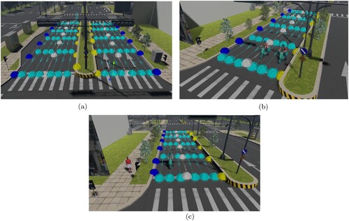
  With the map annotation tool, all four-wheel NPC vehicles should move by following the pre-planned lines, which are pre-arranged with the map annotation tool. In the original design of the SVL simulator, a car line is usually placed at the centre of a lane, as shown in Figure 3(a), which is sufficient for the simulation of four-wheelers, but it is not able to reflect the side-by-side riding style for two-wheelers as shown in Figure 3(b). Hence, we use the annotation tool to draw the lines for two-wheelers, and in our current setup, there are three parallel lines for a scooter to move within a lane. Moreover, it is very likely that two-wheelers may not ride along the pre-defined lines. In order to imitate a free-way riding style, it is important to develop the mechanism that allows a two-wheeler to move along the pre-defined path, which is obtained by the above traffic modelling method. Fortunately, SVL simulator provides the high-level Python APIs to control an NPC object to move along a set of given coordinates (i.e. DriveWaypoint). With the customised paths, we are able to further model the riding styles (Lee & Wong, 2016b) with the 3D simulations to improve the quality of the autonomous driving algorithms, such as collision avoidance; an example of the free riding style is presented in Section 4.4. It is important to note that the four-wheelers follow the centre lines of the lanes, whereas all of the cyan lines are able to be used by two-wheeled vehicles, such as scooters, mopeds, and bicycles.

Figure 3. Illustrations of different scenes on a given map for autonomous vehicle simulations. (a) Illustration of the map annotated with the tracks for four-wheelers. (b) Illustration of two scooters stopped at the stop line side by side and (c) Illustration of a scooter riding at the centre line and a pedestrian walking in the scene.

4. Experimental results

In this section, we describe the setup of our experiments in Section 4.1. The validation result is presented in Section 4.2 to show the functional correctness of using the 3D simulations for the autonomous vehicle development by examining the execution behaviours of the autonomous driving software running in the physical and simulated environments. Section 4.3 presents the results generated by our proposed work for traffic modelling. Section 4.4 demonstrates the applications that can be enabled by our tools to model the motorcycle based traffic scenes in Asia.

4.1. Experimental setup

To validate our developed work, we establish the co-simulation environment for the autonomous vehicle simulation, where the SVL simulator (2019.12 release) is adopted for the 3D simulation and Autoware (version 1.12.0) is used as the autonomous driving software of the simulated self-driving vehicle. The autonomous vehicle equips with the following sensors: a front LiDAR, a front camera, and a GPS/IMU, which are commonly seen sensors for an autonomous vehicle. During the co-simulation, the SVL simulator encapsulates the raw sensor data into the JSON format (RobotWebTools, 2017), which is further converted into the ROS data and is sent to Autoware via rosbridge that is a software module containing the protocol and libraries to exchange data between ROS and non-ROS software systems. As for the implementation of our tool, we find that the software packages in Autoware provide the key functionalities fulfilling our needs for object detection and tracking.¹

The LiDAR sensor data representing the target traffic flows are obtained from two different sources. First, we use the KITTI benchmark suite (Geiger et al., 2013), which is collected by driving the vehicle on a variety of test fields, and the collected sensor data is captured and synchronised at 10Hz, to validate the capability of our tool to classify different types of objects (shown in Section 4.3). Second, to demonstrate the practical usage of our proposed work, we captured the real-world two-wheeler traffic condition, where the LiDAR data records the real-world traffic condition (with two-wheelers) when the physical vehicle drives on the open road. Note that the KITTI dataset is used to validate our developed method since it contains a variety of traffic conditions. As for the modelling of the Southeast Asia-specific traffic, we use the data that we recorded on the physical world.

We create the custom scripts to simulate the recreated traffic flows  (SVL Simulator, 2021). The captured objects are mapped onto the 3D maps of the Shalun in Tainan, Taiwan. In particular, The path of the autonomous vehicle (i.e. the ego vehicle) on the selected maps is captured GPS route. The captured traffic flows of the detected objects are considered NPCs and are mapped onto the designated positions, which overlap the autonomous vehicle's route.

4.2. Validating the 3D simulation

In order to show that the 3D simulation is effective for the autonomous vehicle development, we have done the experiments on both the simulated and physical environments, both of which run the same software stack, including Autoware 1.6.0, ROS kinetic, Ubuntu 16.04 on the same hardware platform equipped with the Intel i7-6700 processor with 16GB memory. The SVL simulator used the 2019.12 release version for doing the 3D simulation. Both of the environments run with the end-to-end lane following mode in ShaLun, as described in Section 4.1. The computation graphs (i.e. rqt_graph) offered by the ROS framework are used to analyse the running software modules of Autoware on the simulated and physical environments. Our experimental results show that Autoware running on the two environments exhibits the same characteristics. That is, the software modules (i.e. ROS nodes) of Autoware from the two environments share similar execution orders; in particular, the same starting modules for receiving the sensor data from both environments,² and different modules to send the driving commands to the simulated and physical vehicles.³

4.3. Extracting moving tracks of classified objects

The traffic modelling methodology described in Section 3.1 has been built and tested with the real-world dataset, KITTI.⁴ This subsection shows the traffic condition of an alley; it is a challenging task for an autonomous vehicle driving through a small alley without incurring collisions while maintaining progress (i.e. moving forward with the proper speed in a small alley). Note that the recorded data contains the movements of pedestrians and cars.

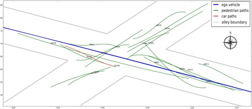
Figure 4 shows a screenshot of the traffic to be modeled and the corresponding LiDAR sensor data. The ego vehicle drives forward and records the LiDAR data, where the black car drives toward the ego vehicle and several pedestrians walk across the alley, which makes the ego vehicle stop at the intersection of the alley. The surrounding situation of the ego vehicle can observe by a bird's eye view of LiDAR data as depicted in Figure 5.  The recognised objects (i.e. a car and pedestrians) and their movement paths are illustrated in Figure 6, where the still objects are removed, which makes the moving patterns more clearer. It is interesting to note that the movements of pedestrians can be classified into two patterns: in the side direction⁵ and in the diagonal direction across the alley. As a result, the captured movements are useful for training an autonomous vehicle for driving through an small alley with pedestrians smoothly.

Figure 4. The input sensor data as illustrated in the step $◯1$ of Figure 2. The top image is the screenshot of the traffic to be modeled, whereas the bottom one is the corresponding LiDAR point cloud.

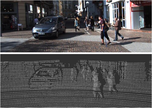
Figure 5. The top-down view of the LiDAR data in Figure 4, where there is a car and several pedestrians in front of the ego vehicle.

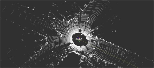
Figure 6. The output generated by object classifying procedure, as illustrated in the step $◯5$ of Figure 2 at the intersection of the alley shown in Figure 5, where different types of the objects, such as ego vehicle (blue line), pedestrians (green lines) and car (red line), are identified and the still objects are removed.

4.4. Applications for modeling Asia traffic

Two-wheelers (e.g. motorcycles and bicycles) are ubiquitous in the urban areas of Asia, such as India, Taiwan, Thailand, and Vietnam. The proposed work helps recreate the Asia-specific traffic conditions. As the two-wheelers are with smaller sizes and with different riding styles, compared with four-wheelers, it is important to train the autonomous vehicles with the riding styles before they drive on Asia roads. Nevertheless, we are not able to find sufficient raw data from KITTI, which contains motor-powered two-wheelers. Here, we show that our work is capable of modelling the two-wheeler-based traffic, and we can import their moving tracks when those data are acquired from the physical world.

4.4.1. Turning Right with Motorcycles

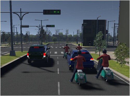
On some Asia's roads, it is common that a vehicle is surrounded by two-wheelers, and the vehicle cannot move until the two-wheelers move, as illustrated in Figure 7. In fact, it is the common case where the traffic accidents occur. For example, it should be considered carefully when the vehicle is about to turn right (right after the traffic light turns green) and some of the two-wheelers are making their moves toward the side way (or go forward). In such a case, the autonomous vehicle (blue car) should anticipate the movements of each surrounding motorcycle and should make its movement carefully so as to avoid collisions. This demands for some special designed algorithm to perform such a task efficiently, e.g. functional correctness and computation efficiency. Our traffic modelling is able to record different traffic scenes on the roads and to recreate the conditions similar to the above case, which will be useful for training the autonomous driving systems.

Figure 7. The autonomous vehicle (blue car) prepares to turn right, together with the motorcycles.

4.4.2. Scooter Riding in the Opposite Direction

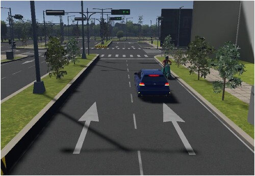
Another common scene on Asia's roads is that a motorcycle may violate the traffic regulation and it goes in the opposite direction against the lane direction, as illustrated in Figure 8. Thus, an autonomous vehicle should be trained beforehand to incorporate with this situation, to drive smoothly and safely, where the simulation-based method provides a safe environment to perform the training before the vehicle runs on the physical environment.

Figure 8. The motorcycle rides in the opposite direction against the autonomous vehicle (blue car).

4.4.3. Motorcycle overtaking

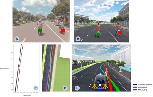
To better illustrate the concept of incorporating the traffic modelling for building a digital twin, we create the traffic scenario of the motorcycle-overtake on the open road,⁶ we record the moving trajectories of the two motorcycles with the LiDAR sensor on the physical vehicle, and we apply the proposed methodology to replicate the moving trajectories of the two motorcycles in the 3D environment. Figure 9 presents the experimental results of the modelling of the two-wheeler traffic. The traffic scenario is that motorcycle B (the left one in Figure 9(a) and (b)) moves to the positions in front of the autonomous vehicle while motorcycle A (the right one in Figure 9(a) and (b)) moves in parallel to the vehicle with different distances as time advances. This scenario helps the development of the driving logic in a crowded traffic condition, where the motorcycles may be very close to the autonomous vehicle. In addition, the autonomous vehicle can learn how to react when a motorcycle may suddenly move in front of it. The screenshot presented in Figure 9(e) represents the time point, where motorcycle B is about to cut in. Note that the motorcycles are moving at the speed of 21.2 km/h and the autonomous vehicle is at 19.8 km/h, which conforms to the settings of the recorded data.⁷ The advantage of the recreation of the traffic conditions is that we can change the speeds of the objects to do the what-if simulations to further improve the knowledge of autonomous driving software.

Figure 9. Two-wheeler traffic modelling with realistic sensor data. (a) and (b) represent the concept of the two-wheeler traffic using the driver view images of the physical and simulated worlds, respectively. (c) and (d) depict the captured and recreated trajectories in (a) and (b), respectively, from the bird view. (e) is the screenshot of the replicated traffic scenario, where the trajectories are pasted on the image to better illustrate the motorcycle-overtake concept.

4.4.4. Performance discussion

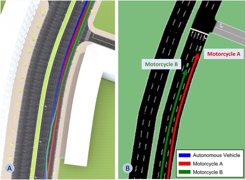
The proposed automatic traffic modelling method enables the capturing and recreating the real-world traffic in the virtual environment, where the related results are exhibited in the above paragraphs. To further differentiate the proposed work against the prior work, we further compare the simulation results offered by our work and SUMO (Simulation of Urban MObility) (Lopez et al., 2018). SUMO is a widely adopted, open-source traffic suite, which is used to simulate large-scale traffic networks, and it can be configured to generate the moving trajectories of the vehicles automatically or manually. Unfortunately, its automatic moving path generation of an NPC vehicle will follow a relatively simple, monotonic trajectory for the traffic network simulation, which cannot reflect the region-specific, real-world traffic. Figure 10 gives a side-by-side comparison of the moving trajectories of the motorcycle overtaking scenario offered by our tool and SUMO. Figure 10(a) exhibits the two motorcycles overtake the ego vehicle, whereas Figure 10(b) depicts that the two motorcycles simply follow the lanes, riding at the centre of the car lanes. It is obvious that the automatic path generation mode provided by SUMO cannot provide such realistic riding styles for the motorcycles since the input parameters for automatic path generations are relatively simple, such as the number of vehicles per hour, and the possibility of going straight and turning right/left. In such a case, the behaviours of the NPC vehicles generated by SUMO are easy to anticipate; that is, it is highly likely that the vehicles change their directions (turning left/right) when encountering the intersections. Furthermore, while SUMO provides a so-called microscopic control for each individual NPC vehicle, it requires its user inputs to provide the movement coordinates of each vehicle, which implies that its users should know the moving trajectories of the NPC vehicles beforehand (and our proposed tool can help bridge the gap). Based on the performance comparison, in terms of the generated moving trajectories, we believe that our proposed work can help facilitate the training of autonomous vehicles by providing real-world traffic in the simulated environment.

Figure 10. The side-by-side performance comparison between our proposed method and SUMO, in terms of the generated moving trajectories for the motorcycle overtaking scenario presented in Figure 9. (a) depicts the traffic scenario captured on the open road and recreated in the simulated environment as shown in Figure 9(d). (b) illustrates the moving trajectories of the two motorcycles generated by SUMO automatically.

5. Conclusion and future work

We present the methodology of modelling the real-world traffic and the design considerations for simulating the modeled traffic condition. Our proposed approach saves the labour costs for modelling different traffic scenes while helping improve the training of driving logics of autonomous vehicles. In the future, we will perform a thorough study to identify representative traffic scenes, to reproduce these scenes in the physical environment, and to validate the obtained results against the realistic data. In addition, we will work on incorporating with different types of sensor data to further model the environmental conditions, as mentioned in Section 3.1.

Disclosure statement

No potential conflict of interest was reported by the authors.

Additional information

Funding

This work is financially supported in part by the ‘Intelligent Manufacturing Research Center’ (iMRC) from The Featured Areas Research Center Program within the framework of the Higher Education Sprout Project by the Ministry of Education (MOE) in Taiwan. This work is also supported by MOE, Taiwan, under the Manpower Cultivation Program of Autonomous Vehicles. This work is supported in part by the Ministry of Science and Technology, Taiwan [grant number MOST-110-2221-E-006-052], [grant number MOST-110-2218-E-006-026].

Notes

1 We leverage the code of the modules to fit our needs, including lidar_euclidean_cluster_detect, native-L-shape fitting, and imm-ukf-pda tracker, which provide good performance (after our analyses) and avoid to reinvent the wheel.

2 For example, the lidar_euclidean_cluster_detect module is used to process the LiDAR data.

3 For instance, vehicle_sender is used to pass the commands to the simulated car, whereas mqtt_bridge_node is called to control the physical car.

4 The data is the city category, and the corresponding file name is 2011_09_29_drive_0071.

5 The green lines are orthogonal to the ego vehicle.

6 It is a dangerous, but common situation for a two-wheeler to cut in front of the vehicle. The coordinate of the experiment is at $\mathrm{N}22{}^{\circ }{55}^{\prime }{44.1}^{″}$ $\mathrm{E}120{}^{\circ }{16}^{\prime }{38.3}^{″}$

7 The demonstration video of the physical and simulated environments is available via the link: https://www.youtube.com/watch?v=2fKgzrVxzLo

References

- Baidu. (2020, August). Apollo website. https://apollo.auto/index.html.
- Blender Online Community. (2018). Blender – a 3D modelling and rendering package [Computer Software Manual]. Stichting Blender Foundation, Amsterdam. http://www.blender.org.
- CARLA. (2020). Carla website. https://carla.org/.
- Cognata. (2020). Cognata website. https://www.cognata.com/simulation/.
- Das, P., & Chand, S. (2021). Extracting road maps from high-resolution satellite imagery using refined DSE-LinkNet. Connection Science, 33(2), 278–295. https://doi.org/10.1080/09540091.2020.1807466
- Geiger, A., Lenz, P., Stiller, C., & Urtasun, R. (2013). Vision meets robotics: The KITTI dataset. International Journal of Robotics Research (IJRR), 32(11), 1231–1237. https://doi.org/10.1177/0278364913491297
- Harper, Jeffrey. (2012). Mastering autodesk 3ds max 2013. John Wiley & Sons.
- Jiang, D., Qu, H., Zhao, J., Zhao, J., & Hsieh, M. Y. (2021). Aggregating multi-scale contextual features from multiple stages for semantic image segmentation. Connection Science, 1–18. https://doi.org/10.1080/09540091.2020.1862059.
- Kato, S., Takeuchi, E., Ishiguro, Y., Ninomiya, Y., Takeda, K., & Hamada, T. (2015, December). An open approach to autonomous vehicles. IEEE Micro, 35(6), 60–68. https://doi.org/10.1109/MM.2015.133
- Lee, T. C., & Wong, K. (2016a). An agent-based model for queue formation of powered two-wheelers in heterogeneous traffic. Physica A: Statistical Mechanics and Its Applications, 461, 199–216. https://doi.org/10.1016/j.physa.2016.05.005
- Lee, T. C., & Wong, K. I. (2016b, November). An agent-based model for queue formation of powered two-wheelers in heterogeneous traffic. Physica A: Statistical Mechanics and Its Applications, 461, 199–216. https://doi.org/10.1016/j.physa.2016.05.005
- Liu, Y., Wang, Z., Han, K., Shou, Z., Tiwari, P., & Hansen, J. H. L. (2020). Sensor fusion of camera and cloud digital twin information for intelligent vehicles. 2020 IEEE Intelligent Vehicles Symposium (IV), Las Vegas, NV, USA, 19 Oct.-13 Nov. 2020. https://doi.org/10.1109/IV47402.2020.9304643
- Lopez, P. A., Behrisch, M., Bieker-Walz, L., Erdmann, J., Flötteröd, Y. P., Hilbrich, R., Lücken, L., Rummel, J., Wagner, P., & Wießner, E. (2018). Microscopic traffic simulation using SUMO. In The 21st IEEE International Conference on Intelligent Transportation Systems. IEEE. https://elib.dlr.de/124092/.
- Nvidia. (2020). Nvidia drive constellation website. https://www.nvidia.com/en-us/self-driving-cars/drive-constellation/.
- Pell, A., Meingast, A., & Schauer, O. (2017). Trends in real-Time traffic simulation. Transportation Research Procedia, 25(1B), 1477–1484. https://doi.org/10.1016/j.trpro.2017.05.175
- PTV Group. (2021). PTV Vissim website. https://www.ptvgroup.com/en/solutions/products/ptv-vissim/.
- Rachman, A. S. A. (2017). 3d-lidar multi object tracking for autonomous driving: Multi-target detection and tracking under urban road uncertainties [Master's thesis]. Mekelweg 5, 2628 CD, Delft, Netherlands: Delft University of Technology.
- rFpro. (2020). rfpro website. http://www.rfpro.com/.
- RobotWebTools. (2017, October). rosbridge_suite website. http://wiki.ros.org/rosbridge_suite.
- Rodrigues, L., Neto, F., Gonçalves, G., Soares, A., & Silva, F. A. (2021). Performance evaluation of smart cooperative traffic lights in VANETs. International Journal of Computational Science and Engineering, 24(3), 276–289. https://doi.org/10.1504/IJCSE.2021.115650
- Rong, G., Shin, B. H., Tabatabaee, H., Lu, Q., Lemke, S., Možeiko, M., Boise, E., Uhm, G., Gerow, M., Mehta, S., Agafonov, E., Kim, T. H., Sterner, E., Ushiroda, K., Reyes, M., Zelenkovsky, D., & Kim, S. (2020). LGSVL simulator: A high fidelity simulator for autonomous driving. 2020 IEEE 23rd International Conference on Intelligent Transportation Systems (ITSC), Rhodes, Greece, 20-23 Sept. 2020. https://doi.org/10.1109/ITSC45102.2020.9294422
- SVL Simulator. (2021, September). Svl simulator document. https://www.svlsimulator.com/docs/python-api/python-api/#npc-vehicles.
- Wang, Z., Han, K., & Tiwari, P. (2021). Digital twin simulation of connected and automated vehicles with the unity game engine.
- Wismans, L., de Romph, E., Friso, K., & Zantema, K. (2014). Real time traffic models, decision support for traffic management. Procedia Environmental Sciences, 22(3), 220–235. https://doi.org/10.1016/j.proenv.2014.11.022
- Xu, R., Guo, Y., Han, X., Xia, X., Xiang, H., & Ma, J. (2021). OpenCDA: An open cooperative driving automation framework integrated with co-simulation. 2021 IEEE International Intelligent Transportation Systems Conference (ITSC), Indianapolis, IN, USA, 19-22 Sept. 2021. https://doi.org/10.1109/ITSC48978.2021.9564825
- Yao, J., Dai, Y., Ni, Y., Wang, J., & Zhao, J. (2020). Deep characteristics analysis on travel time of emergency traffic. International Journal of Computational Science and Engineering, 22(1), 162–169. https://doi.org/10.1504/IJCSE.2020.107271
- Zhang, H., Wang, X., Luo, X., Xie, S., & Zhu, S. (2021). Unmanned surface vehicle adaptive decision model for changing weather. International Journal of Computational Science and Engineering, 24(1), 18–26. https://doi.org/10.1504/IJCSE.2021.113634
- Zhang, X., Xu, W., Dong, C., & Dolan, J. M. (2017, June). Efficient L-shape fitting for vehicle detection using laser scanners. 2017 IEEE Intelligent Vehicles Symposium (IV), Los Angeles, CA, USA, 11-14 June 2017. https://doi.org/10.1109/IVS.2017.7995698
- Zhao, H., Yao, L., Zeng, Z., Li, D., Xie, J., Zhu, W., & Tang, J. (2021). An edge streaming data processing framework for autonomous driving. Connection Science, 33(2), 173–200. https://doi.org/10.1080/09540091.2020.1782840