Robust coal granularity estimation via deep neural network with an image enhancement layer

Abstract

Accurate granularity estimation of ore images is vital in automatic geometric parameter detecting and composition analysis of ore dressing progress. Machine learning based methods have been widely used in multi-scenario ore granularity estimation. However, the adhesion of coal particles in the images usually results in lower segmentation accuracy. Because much powdery coal fills between blocky ones, making edge contrast between them is not distinct. Currently, the coal granularity estimation is still carried out empirical in nature. We propose a novel method for coal granularity estimation based on a deep neural network called Res-SSD to deal with the problem. Then, to further improve the detection performance, we propose an image enhancement layer for Res-SSD. Since the dust generated during production and transportation will seriously damage the image quality, we first propose an image denoising method based on dust modelling. By investigating imaging characteristics of coal, we second propose the optical balance transformation(OBT), by which the distinguishability of coal in dark zones can be increased. Meanwhile, OBT can also suppress overexposed spots in images. Experimental results show that the proposed method is better than classic and state-of-the-art methods in terms of accuracy while achieving a comparable speed performance.

Keywords:

• Coal granularity estimation
• deep neural network
• dust removal
• image enhancement
• industrial and mining intelligence

1. Introduction

At present, the majority of plants directly send crude coal into the coal preparation equipment. Because most coal mines are mining at multiple working faces with different geological structures, the quality and granularity of crude coal fluctuate considerably (Belov et al., 2020; Gui et al., 2021).

As a result, the coal preparation plant has to face the situation of uneven quality and granularity in the process of coal supplying, transportation, separating, and washing. It seriously threatens the operation safety of relevant equipment, such as the jamming of coal suppliers and transfer chute, the damage of transportation belt, and the deformation of the scraper of shallow trough separator (Zhang & Deng, 2019). Moreover, crude coal with uneven granularity also leads to severe fluctuations in the processing capacity of various equipment. The system processing capacity can not reach the design value or be maximised, thus reducing the production efficiency (Yang et al., 2019).

Unfortunately, due to the limitations of application scenarios, the coal granularity estimation is still carried out empirical in nature. Some plants install vibration sieves. Samples are taken at regular intervals, and the coal granularity is obtained from the screening results observed by workers. Other factories arrange workers to always pay attention to the instantaneous current of the conveyor belt to predict the belt load. Under the assumption that the discharge is stable, the coal granularity is estimated by personal experience. There is no doubt that human experience cannot be quantified, and long hours of monotonous work can easily make workers tired and slack. In the light of the current situation, we propose a robust coal granularity estimation method based on a deep neural network with an image enhancement layer. The main contributions of this paper can be summarised as follows.

1. Starting from the principle of coal imaging, we deeply investigated the key issues and reasons for the coal granularity estimation task.

2. We propose a deep neural network structure named Res-SSD to detect the coal in images and achieve a competitive result to other approaches.

3. We build an image enhancement layer for the proposed Res-SSD. It contains a dust removal method and an optical balance transform. The layer can solve the problem of insufficient image quality caused by dust and significantly improve the distinguishability of coal in the images.

4. We carry out experiments and evaluate the accuracy and speed performance on a large database. The results demonstrate the effectiveness of the proposed method.

The remainder of this paper is organised as follows. Since in recent years, it seems that the research on this topic has reached a bottleneck. Section 2 briefly introduces the related works, namely, existing ore detection/segmentation methods. Then, we concentrate on the differences between this topic and previous approaches to explain the particularity of our task. Section 3 presents our deep neural network structure Res-SSD. In this section, although we prove that Res-SSD achieved a better performance than other methods, the results also show that we should further improve the proposed method to better complete the task of granularity estimation. Therefore, in Section 4, we build an image enhancement layer. The layer could remove the dust and enhance the distinguishability of coal in the image. Section 5 gives our experimental results and analysis. Section 6 offers our conclusion.

2. Related works

Existing research on automatic ore granularity estimation or analysis can be roughly classified into traditional and artificial intelligence based methods.

Traditional methods usually make use of additional mechanical components or physical properties of materials, such as vibrating screen (Ye, 2018), density analysis (Hu & Nikolaus, 2017; Rubey, 1933), ultrasonic measurement (Allegra et al., 1972), laser measurement (Luo et al., 2013), etc. These methods are subject to the working life of the equipment, especially in industrial and mining plants with a poor working environment. Besides, these methods have low accuracy and poor adaptability (Duan et al., 2020; Zhang et al., 2011).

With the rapid development of image processing technology and machine learning in recent years, artificial intelligence based methods began to be applied in this field. Some tried to make segmentation by edge-like features (Chen & Zhang, 2020; Purswani et al., 2020; Zhou & Hui, 2012). In 2012, Zhang et al. (2012) proposed a bimodal threshold based method and improved it later in Zhang et al. (2013). They segmented the targets and estimated coal granularity by fitting target circumscribed rectangle. However, this method requires objects to be discrete and not adjacent. Besides, it has high computational complexity and low application value. Recently, Zhan and Zhang (2019) proposed an ore image segmentation algorithm based on histogram accumulation moment and demonstrated its effectiveness in multi-scenario ore object location and recognition. In Zhang et al. (2011), Wei and Jiang (2011) and Amankwah and Aldrich (2011), researchers applied the watershed algorithm to segment ore images. Nevertheless, these methods are sensitive to parameters selection and image quality (Wang et al., 2021).

Benefit from the powerful recognition ability of the deep neural network. Xiao et al. (2020) proposed a DU-Net based structure, RDU-Net, to estimate ore fragment size. In Liu et al. (2020), a similar net structure combined U-Net and ResU-Net was proposed. Compared with U-Nnet, the method improved model sensitivity to misclassified pixels, pixels of similar appearance, and pixels near the boundary. Yang et al. (2021) proposed a contour awareness loss (CAL). Existing deep neural network based methods have achieved better results in ore detection and granularity estimation. However, the detection targets of these methods mainly focus on ores (aluminium ore, iron ore, etc.) and rocks.

In 2020, Zhang et al. (2020) proposed a method to detect coal quality multi-information, including granularity. Their work was a bench-scale approach. The coal is completely separated on the testing platform with a clean detection environment. Bai et al. (2021) employed a series of segmentation methods, including the watershed and k-nearest, to achieve preliminary segmentation and merge small pieces with large pieces. Finally, the granularity information was output by calculating the areas of pieces. This method did not consider the influence of powdery coal so that the edge of coal in the test images is clear and distinct. Compared with other kinds of ore, e.g. iron or aluminium, coal is harder to detect in practical application scenarios, and the detection task is far from being resolved. We have analysed the four main reasons as follows.

1. The colour or grayscale of coal is not rich in an image. Besides, the colour of adjacent materials is very close. Hence, the boundary between them is not distinct.

2. Generally, coal has two physical states: blocky and powder. The powdery coal is filled among the blocky ones, making the boundary less distinguishable.

3. Powdery coal has strong light absorption characteristics (Sun et al., 2017) and makes the part it belongs to darker. We name the part as a dark zone. On the contrary, the blocky coal shares many similarities with crystals, and there are some overexposed spots caused by specular reflection.

4. Due to the existence of powdery coal, they will produce a lot of dust during transportation(e.g. on a belt conveyor), resulting in severe image blurring.

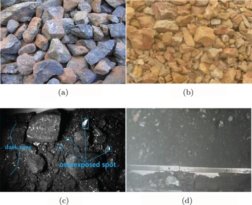
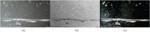
Figure 1 shows some examples of different kinds of ores. We can see those iron ores in Figure 1(a) and aluminium ores in Figure 1(b) are blocky, which the boundary is quite clear. However, Figure 1(c) illustrates some blocky coal surrounded even covered by powdery coal, making their boundary not distinct. Figure 1(d) shows coal on a working belt conveyor. The dust of powdery coal blurred the image seriously.

Figure 1. Examples of different kinds of ores. (a) Iron ore, (b) aluminium ore, (c) coal and (d) coal in transportation.

3. Coal detection using Res-SSD

3.1. Res-SSD

Since it is difficult to choose or build structural features for coal, deep neural network based methods are more suitable for coal detection or granularity estimation. Because deep neural network could automatically extract and abstract the correlation of high-dimensional data layer by layer (Jiang et al., 2021; Wu et al., 2019; Xiao et al., 2020; Xu & Zhang, 2020; Zhu et al., 2020).

Considering that the primary purpose of coal granularity estimation is engineering application in practice, we build a one-stage deep-neural net structure named Res-SSD to trade-off between accuracy and speed.

SSD (Liu et al., 2016) employs VGG (Sengupta et al., 2019) network as the backbone to extract shallow features. Then, it extracts further features by adding four groups of convolution layers. Different layers predict the positions and categories of objects, and the final detection results are obtained under loss threshold and non-maximum suppression. We replace VGG with a residual network (He et al., 2016) as the backbone. More specifically, as SSD uses the former five blocks of VGG-16 and then outputs the first detection results at 4−3rd layer, we perform the former four blocks of ResNet-101 to replace the VGG-16. The structure of the proposed Res-SSD is shown in Figure 2. The first detection results are output in layer 4−3rd layer. Table 1 lists the kernels' sizes of selected four blocks in ResNet101, i.e. conv_x to conv_4x in Figure 2.

Figure 2. Structure of proposed Res-SSD.

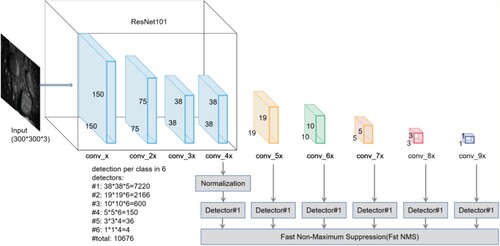
Table 1. Applied kernels of ResNet101 in the proposed Res-SSD.

Layer	Output size	Kennel size
conv_x	$150\times 150$	$7\times 7$, 64
conv_2x	$75\times 75$	$\left[\begin{array}{cc}1\times 1,& 64\\ 3\times 3,& 64\\ 1\times 1,& 256\end{array}\right]\times 3$
conv_3x	$38\times 38$	$\left[\begin{array}{cc}1\times 1,& 128\\ 3\times 3,& 128\\ 1\times 1,& 512\end{array}\right]\times 4$
conv_4x	$38\times 38$	$\left[\begin{array}{cc}1\times 1,& 256\\ 3\times 3,& 256\\ 1\times 1,& 1024\end{array}\right]\times 23$

For different object detectors in Figure 2, they have different sizes of feature maps and receptive fields. To this end, we adopt an adaptive detection box for various sizes of objects. It makes our network could find different sizes of coal and estimate the granularity in one image. As we have k kinds of feature maps to detect the object, the default size $S_i$ in ith feature map is set as Equation (1(1) $S_i=\alpha +\frac{\text{β}-\alpha }{k-1}(i-1),i\in [1,k],$(1) ). (1) $S_i=\alpha +\frac{\text{β}-\alpha }{k-1}(i-1),i\in [1,k],$(1) where $\alpha =0.30$ and $\text{β}=0.95$ are the minimum and maximum scales of the boxes. We perform several aspect ratios ar as $ar\in \{1/3,1/2,1/1,2/1,3/1\}$ to meet the requirements of different shapes of boxes. In this manner, the default width $w_i$ and height $h_i$ of the ith box can be calculated by Equation (2(2) $\{\begin{array}{l}{w}_i=\sqrt{ar\cdot S_i}\\ h_i=\sqrt{\frac{S_i}{ar}}\end{array},ar\in \{\frac{1}{3},\frac{1}{2},1,2,3\}.$(2) ). (2) $\{\begin{array}{l}{w}_i=\sqrt{ar\cdot S_i}\\ h_i=\sqrt{\frac{S_i}{ar}}\end{array},ar\in \{\frac{1}{3},\frac{1}{2},1,2,3\}.$(2) In the training stage, a labelled box may match several default boxes. At first, the proposed method selects one default box that obtains the maximum value of intersection-over-union (IoU) to build the corresponding relationship with the labelled box. Then, the remaining default boxes will find their corresponding relationship if the IoU values exceed the predefined threshold $s_{IoU}=0.45$. This procedure helps the model learn the scene in which one labelled target matches with more than one detection box.

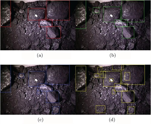
Figure 3 illustrates the comparison results of YOLOv3 (Redmon & Farhadi, 2018), RDU-Net (Xiao et al., 2020), ResU-Net (Liu et al., 2020), and proposed Res-SSD. We can see that the proposed Res-SSD achieves a better result than other methods in coal detection. However, due to the low distinguishability of coal in the image, the recognition accuracy still needs to be further improved, especially for low contrast areas, i.e. dark zones. Besides, the proposed method incorrectly detected some overexposed areas as independent targets.

Figure 3. Detection results of different deep neural networks. (a) YOLOv3, (b) RDU-Net, (c) ResU-Net and (d) Res-SSD.

3.2. Coal granularity estimation based on detection results

For practical application scenarios, it is unnecessary to calculate full-band granularity values. Usually, we only need to get the distribution of granularity in several intervals. Generally, coal is considered to have three granularity levels. In a coal washing plant, the fine level means that the coal can be washed directly; the medium level means that the plant's production capacity should be paid attention to when washing coal; the large level means that extensive of this kind of coal may damage plant equipment, and the quantity needs to be strictly controlled. Different plants have different requirements, which are mainly according to the design processing capacity of the equipment.

We put a target with standard size on the conveyor belt (e.g. cigarette box or A4 paper) and then obtain its size (pixels) in the image to obtain the corresponding relationship. Table 2 gives the dimension relationship applied in our practical application and experiments. When we get the coal detection results based on the proposed Res-SSD, we can calculate the areas of each rectangle box, and then find the corresponding granularity levels in this table. For detection results, the undetected part is usually defined as background. While for this task, there are only different forms of coal (blocky and powdery) to detect. We can ensure this by setting the region of interest (ROI). In the manual annotation stage, only the medium and sizeable blocky coal are labelled. To this end, one detected object must belong to a medium or large granularity level. The undetected part is classified into the fine level, which is composed of powdery and small blocky coal.

Table 2. Dimension correspondence.

Granularity level	Granularity/${\mathrm{c}\mathrm{m}}^2$	Area in image/pixel
Fine	$(0,30\times 30]$	$(0,75\times 75]$
Medium	$(30\times 30,100\times 100]$	$(75\times 75,250\times 250]$
Large	$(100\times 100,+\mathrm{\infty }]$	$(250\times 250,+\mathrm{\infty }]$

From Figure 3, we can see the detection performance still needs to be further improved. Therefore, we build an image enhancement layer to estimate the coal granularity more robustly.

4. Image enhancement layer

From the discussion in previous sections, we apply image enhancement in two ways: removing dust and improving the distinguishability of coal in the image. Hence, the image enhancement layer can be treated as a preprocessing stage before sending the input image into the proposed Res-SSD. We will present our method in detail in this section.

4.1. Image denoising based on dust modeling

The impact of dust on the image is similar to that of fog or haze. Inspired by He and Tang (2010, 2012), we can imitate the haze model to build the dust model as: (3) $O\left(x\right)=J\left(x\right)d\left(x\right)+I(1-d(x\left)\right),$(3) where $O\left(x\right)$ and $J\left(x\right)$ are observed image and dust removal images. $d\left(x\right)$ and I refer to the dust model and illumination model, respectively. Hence, if we can obtain $d\left(x\right)$ and I, the dust removal image can be deduction by Equation (4(4) $d\left(x\right)=\frac{I-O\left(x\right)}{I-J\left(x\right)}.$(4) ). (4) $d\left(x\right)=\frac{I-O\left(x\right)}{I-J\left(x\right)}.$(4) It is obvious that $d\left(x\right)$ satisfies $d\left(x\right)\in [0,1]$ and the value range of $O\left(x\right)$, $J\left(x\right)$ and I is $[0,255]$. Since the illumination model I is not affected by object occlusion and dust, we can determine an inequality as Equation (5(5) $0\le O\left(x\right),J\left(x\right)\le I.$(5) ). (5) $0\le O\left(x\right),J\left(x\right)\le I.$(5) From Equations (4(4) $d\left(x\right)=\frac{I-O\left(x\right)}{I-J\left(x\right)}.$(4) ) and (5(5) $0\le O\left(x\right),J\left(x\right)\le I.$(5) ), we can derive another inequality as Equation (6(6) $\begin{array}{rl}d\left(x\right)& \ge \frac{I-O\left(x\right)}{I-0}=\frac{I-O\left(x\right)}{I}=1-\frac{O\left(x\right)}{I}.\end{array}$(6) ). Therefore, the illumination model $d\left(x\right)$ satisfies Equation (7(7) $\begin{array}{rl}1-\frac{O\left(x\right)}{I}& \le d\left(x\right)\le 1.\end{array}$(7) ). (6) $\begin{array}{rl}d\left(x\right)& \ge \frac{I-O\left(x\right)}{I-0}=\frac{I-O\left(x\right)}{I}=1-\frac{O\left(x\right)}{I}.\end{array}$(6) (7) $\begin{array}{rl}1-\frac{O\left(x\right)}{I}& \le d\left(x\right)\le 1.\end{array}$(7) To model $d\left(x\right)$, rewrite Equation (7(7) $\begin{array}{rl}1-\frac{O\left(x\right)}{I}& \le d\left(x\right)\le 1.\end{array}$(7) ) as (8(8) $d\left(x\right)=\alpha (1-\frac{O\left(x\right)}{I}).$(8) ), where α is a constant with $0\le \alpha \le 1$. $\alpha =0$ only if there is no dust in the observed image, i.e. $O\left(x\right)=J\left(x\right)$. (8) $d\left(x\right)=\alpha (1-\frac{O\left(x\right)}{I}).$(8) For our task, environmental illumination can be regarded as well-distributed and uniform (Sun et al., 2021). From the method in Zhu et al. (2015), the uniform environment illumination model satisfies Equation (9(9) $min\left(\underset{c\in r,g,b}{min}\right(im{g}^c\left(x\right)\left)\right)\le I\le max\left(\underset{c\in r,g,b}{max}\right(im{g}^c\left(x\right)\left)\right),$(9) ). 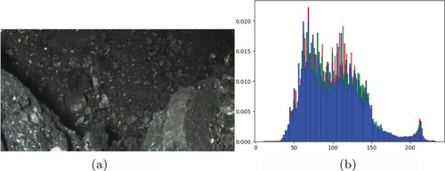(9) $min\left(\underset{c\in r,g,b}{min}\right(im{g}^c\left(x\right)\left)\right)\le I\le max\left(\underset{c\in r,g,b}{max}\right(im{g}^c\left(x\right)\left)\right),$(9) where $im{g}^c\left(x\right)$ represents different colour channels, i.e. red, green, and blue. The colour distributions of background and targets in a coal image are pretty similar, as shown in Figure 4. The histogram distribution of each colour channel is very similar, just like a gray image. It demonstrates the declaration in Section 2 that the coal image lacks colour information.

Figure 4. An example of coal image and its colour histogram distribution, in which the different colours of bins represent corresponding image channels. (a) Input and (b) histogram of the input.

Therefore, obtaining I by Equation (9(9) $min\left(\underset{c\in r,g,b}{min}\right(im{g}^c\left(x\right)\left)\right)\le I\le max\left(\underset{c\in r,g,b}{max}\right(im{g}^c\left(x\right)\left)\right),$(9) ) makes no sense. Fortunately, our observation shows that the dust image shares similar characters with heavily blurred images by an average filter. To this end, we simulate the environmental illumination I by modifying Equation (9(9) $min\left(\underset{c\in r,g,b}{min}\right(im{g}^c\left(x\right)\left)\right)\le I\le max\left(\underset{c\in r,g,b}{max}\right(im{g}^c\left(x\right)\left)\right),$(9) ) as (10(10) $min\left(Ave\right(img\left(x\right)\left)\right)\le I\le max\left(Ave\right(img\left(x\right)\left)\right),$(10) ). (10) $min\left(Ave\right(img\left(x\right)\left)\right)\le I\le max\left(Ave\right(img\left(x\right)\left)\right),$(10) where $Ave(\bullet )$ refers to a $5\times 5$ average filter. Figure 5 shows our results of the dust removal method.

Figure 5. The results of our dust removal method. (a) Input, (b) dust model and (c) dust-free image.

4.2. Optical balance transformation

Coal images may contain dark zones and overexposed spots. The dynamic range is narrow in dark zones, making the objects not distinct. Overexposed spots may lead to wrong segmentation/detection results (Kholerdi et al., 2016), because a spot with a significant brightness difference from the adjacent part is quite possible to be detected as an independent separate, even if it belongs to a flat area. Therefore, this task can be described as how to handle optical imbalance on the surface of coal images. We transfer it into two sub-issues: broadening the dynamic range in dark zones and restraining the high-brightness parts simultaneously. This subsection will introduce an optical balance transformation (OBT) in detail.

An overexposed spot can be regarded as a small high-brightness area which randomly distributed. The overexposed spot is a special kind of salt $\mathrm{\&}$ pepper noise from our observation. More precisely, overexposed spots are pure salt noise with different sizes. Many classic filters (Nader et al., 2017; Tang et al., 1995) could handle salt $\mathrm{\&}$ pepper noise. Rather than filtering the image using a fixed-size sliding window, we employ several adaptive size windows. Figure 6 illustrates a simplified procedure and results for removing overexposed spots.

Figure 6. The overexposed spots removal. (a) Input, (b) binary image, (c) adaptive-size filters and (d) result.

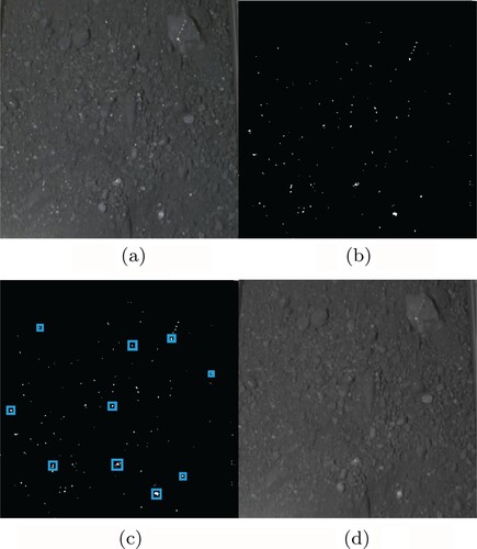
For the input image in Figure 6(a), we can easily locate the overexposed spots by image binarization, as shown in Figure 6(b). Then we employ different sizes of filters for each connected domain. Figure 6(c) shows some positions of filters with different sizes. Under the assumption that one overexposed spot belongs to a regular part nearby, we propose an improved median filter to obtain the results, as shown in Figure 6(d).

First, find the median δ in an $M\times M$ window at the position $(i,j)$ by Equation (11(11) $\begin{array}{rl}\delta & =median\left(\sum _{i=1}^M\sum _{j=1}^{M}img\right(i.j\left)\right),\end{array}$(11) ). The value of M is determined by Equation (12(12) $\begin{array}{rl}M& =\hat{M}+\lambda .\end{array}$(12) ), where $\hat{M}$ is the square's side length circumscribed by a specific connected domain. λ is an integer, and we use $\lambda =3$ in our experiments and practice. (11) $\begin{array}{rl}\delta & =median\left(\sum _{i=1}^M\sum _{j=1}^{M}img\right(i.j\left)\right),\end{array}$(11) (12) $\begin{array}{rl}M& =\hat{M}+\lambda .\end{array}$(12) Then, we reassign all the pixel values in the $(i,j)$ centred filter according to Equation (13(13) $img(m,n)=\{\begin{array}{l}img(m,n),ifimg(m,n)<k\delta ,\\ Avg(m,n),ifimg(m,n)\ge k\delta Avg(m,n)<k\delta ,\\ k\delta ,otherwise,\end{array}$(13) ). The constant k is to adjust the overall brightness of the image. (13) $img(m,n)=\{\begin{array}{l}img(m,n),ifimg(m,n)<k\delta ,\\ Avg(m,n),ifimg(m,n)\ge k\delta Avg(m,n)<k\delta ,\\ k\delta ,otherwise,\end{array}$(13) where $(m,n)$ represents each pixel in the $(i,j)$ centred filter window and $Avg(m,n)$ is the average value obtained by a $3\times 3$ sub-window, centred at $(m,n)$. Therefore, the filtering procedure changes all the pixel values rather than the single-pixel value $img(i,j)$ according to Equation (13(13) $img(m,n)=\{\begin{array}{l}img(m,n),ifimg(m,n)<k\delta ,\\ Avg(m,n),ifimg(m,n)\ge k\delta Avg(m,n)<k\delta ,\\ k\delta ,otherwise,\end{array}$(13) ).

In addition to overexposed spots removal, we have to broaden the dynamic range in dark zones. Hence, we present a two-stage image transformation as Equation (14(14) $$\begin{gathered} img(i,j)= \\ \{\begin{array}{l}V{\left({\displaystyle \frac{img(i,j)}{V}}\right)}^{\frac{1}{\gamma }},ifimg(i,j)<\delta ,\\ \frac{V-V(\frac{\delta }{V}{)}^{\frac{1}{\gamma }}}{V-\delta }\left(img\right(i,j)-\delta )+V{\left({\displaystyle \frac{\delta }{V}}\right)}^{\frac{1}{\gamma }},otherwise.\end{array} \end{gathered}$$(14) ). It is a piecewise function composed of an exponential transformation applied in dark zones and a linear transformation applied in other parts. The exponential transformation could enlarge the dynamic range for the image (Farid, 2001), while the linear transformation restrains the high-brightness parts. (14) $$\begin{gathered} img(i,j)= \\ \{\begin{array}{l}V{\left({\displaystyle \frac{img(i,j)}{V}}\right)}^{\frac{1}{\gamma }},ifimg(i,j)<\delta ,\\ \frac{V-V(\frac{\delta }{V}{)}^{\frac{1}{\gamma }}}{V-\delta }\left(img\right(i,j)-\delta )+V{\left({\displaystyle \frac{\delta }{V}}\right)}^{\frac{1}{\gamma }},otherwise.\end{array} \end{gathered}$$(14) In this function, $\gamma =2.3$ is used to control the shape of the exponential curve, and δ refers to the median value of the input image. V = 255 is the maximum value of pixels. The curve of the proposed transformation is illustrated in Figure 7.

Figure 7. Two-stage transformation.

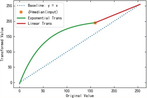
Figure 8 shows the results of image enhancement by the proposed OBT algorithm. We can see that the coal in the dark zones at the four corners of Figure 8(b) is more distinct than that in Figure 8(a). Meanwhile, the overexposed spots are removed. Therefore, we can state that the OBT algorithm could effectively correct the optical imbalance in an image.

Figure 8. Results of OBT algorithm. (a) Original image and (b) enhanced image.

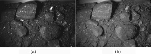
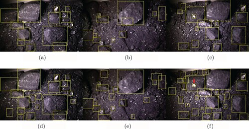
Figure 9 gives three examples of the comparison results. Figure 9(a–c) are detection results of Res-SSD. Figure 9(d–f) are corresponding results of Res-SSD with the proposed enhancement layer, respectively. For results in Figure 9(d–f), we also use enhanced images in the training stage. The results illustrate that the image enhancement layer improves the Res-SSD to detect more objects, especially those in dark zones with low contrast. We also recognise that the proposed method still misses some targets. Besides, it fails to remove some unique overexposed spots, as shown in Figure 9(f), marked by a red arrow. We have investigated the reason as follows. We assume that the overexposed pixels are located at the centre for a square-shaped filter, and the surrounding pixels belong to the regular part. From top-left to bottom-right, the filter operates each pixel through a tiny-sized ($3\times 3$) sliding window. If the sliding window is full of overexposed pixels in the initial steps, our method will fail. We can reduce the probability of this problem by expanding the sliding or filter window size, but we have to bear a larger amount of calculation.

Figure 9. Comparison results of Res-SSD with (+) and without (−) the enhancement layer. (a) Sample A−, (b) Sample B−, (c) Sample C−, (d) Sample A+, (e) Sample B+ and (f) Sample C+.

5. Experimental results

In this section, we implement experiments to evaluate the proposed method in terms of speed and accuracy. The experiments are carried out on a personal computer with Geforce GTX 1080TI GPU, Intel i7-8700 3.20 GHz CPU, and 8 GB RAM. All the comparison methods are applied on the same testing platform. The proposed testing programs are written in Python language. The experimental database comprises 5000 images collected from five coal mines in eastern Inner Mongolia, China. The coal quality of these coal mines is close, and the difference of samples is mainly concentrated in the detection environment of the plants. About $20\mathrm{\%}$ of images contain varying degrees of dust. We randomly split the experimental database into three subsets. Training database (TR-DB) contains 1000 images, validation database (V-DB) and testing database (T-DB) contain 500 and 3500 images, respectively. The experimental results in this section are the average values obtained from five testing procedures.

5.1. Parameters selection

In the training stage, we set batch-size=64. The initial learning rate is specified as $10\times {10}^{-4}$ and be updated adaptively by the RMSProp method (Zou et al., 2019). The maximum number of iterations is 20,000. The other parameters not mentioned in this subsection are chosen as the default values in the relevant literature for comparison methods.

5.2. Detection performance of proposed method

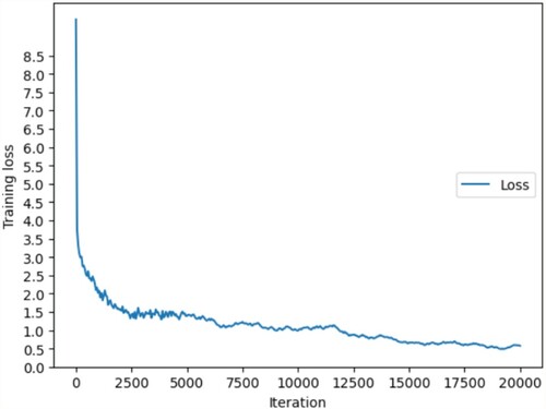
The curve of training loss represents a trend of model convergence. It can also represent the training process of a model in the training database. Figure 10 shows the training loss curve of the proposed method. We can see that with the increase of iterations, the training loss gradually decreases and tends to be stable in the range of 0.5−1.0. That is, the proposed model achieves convergence after almost 17,500 iterations.

Figure 10. Training loss curve of proposed method.

P-R(Precision-Recall) curve is one of the most critical indicators to evaluate the accuracy performance of a model, where $\mathit{p}\mathit{r}\mathit{e}\mathit{c}\mathit{i}\mathit{s}\mathit{i}\mathit{o}\mathit{n}$ refers to the proportion of correctly detected targets in all detected targets and $\mathit{r}\mathit{e}\mathit{c}\mathit{a}\mathit{l}\mathit{l}$ refers to the ratio of detected targets in all ground-truth targets of an image. We can obtain them by Equations (15(15) $\begin{array}{rl}precision& =\frac{TP}{TP+FP},\end{array}$(15) ) and (16(16) $\begin{array}{rl}recall& =\frac{TP}{TP+FN},\end{array}$(16) ). (15) $\begin{array}{rl}precision& =\frac{TP}{TP+FP},\end{array}$(15) (16) $\begin{array}{rl}recall& =\frac{TP}{TP+FN},\end{array}$(16) where TP is true-positive rate, FP and FN are false-positive rate and false-negative rate, respectively. The P-R curve of the proposed method is shown in Figure 11.

Figure 11. P-R curve of proposed method.

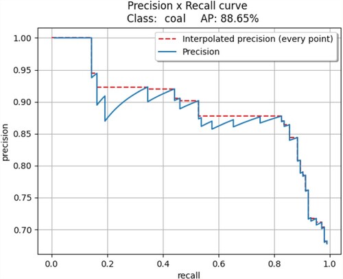
We present two types of precision indicators in the figure. The first one is a point-to-point precision value corresponding to a discrete recall value. The second one is called interpolated precision which is adopted by many approaches (He et al., 2016; Redmon & Farhadi, 2018; Sengupta et al., 2019). It takes the maximum value of the first indicator from the origin to the current position. We can obtain it from Equation (17(17) $P\left(k\right)=\underset{k\ge \hat{k}}{max}P\left(\hat{k}\right),$(17) ). (17) $P\left(k\right)=\underset{k\ge \hat{k}}{max}P\left(\hat{k}\right),$(17) where $P\left(k\right)$ is the interpolated precision value at the position of recall = k. Furthermore, we can obtain the average precision(AP) as Equation (18(18) $P\left(k\right)={\int }_0^{1}P\left(k\right)\mathrm{d}k.$(18) ). (18) $P\left(k\right)={\int }_0^{1}P\left(k\right)\mathrm{d}k.$(18) In Figure 11, the value of AP is the area enclosed of recall value and interpolated precision value, that is, the area of the P-R curve. AP value can indicate the accuracy performance of a model. On T-DB, the proposed method achieves AP=$88.65\mathrm{\%}$.

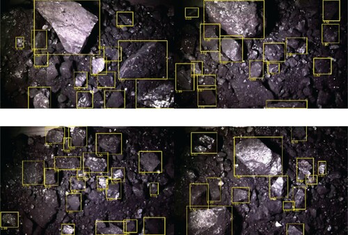
Figure 12 shows some examples of the detection results of the proposed method on T-DB. In these examples, the confidence is set as $50\mathrm{\%}$, and the threshold of the side length of a detection box is set as 75 pixels (corresponding to the fine granularity level as introduced in Table 1).

Figure 12. Detection results of proposed method.

In practical application, we transplant our method on Hisilicon Hi3559 based platform. It has 4GB DDR4 RAM, 16GB eMMC, and NNIE$@$840MHz with a core duo neural network acceleration engine. From the testing results over 24 months, we achieved a frame rate (frame per second, FPS) of 10.2 FPS. The speed of the belt conveyor is about 4m$/$s in general, and the viewing field of the applied camera covers more than 5 m of the belt. It demonstrated that the proposed method could achieve real-time detection (granularity estimation) and full-scene coverage.

5.3. Comparisons and analysis

To make a fair comparison, we choose several object detection approaches and estimate coal granularity by the proposed method in Section 3.2. The comparison methods include two state-of-the-art ore detection methods, namely RDU-Net (Xiao et al., 2020), ResU-Net (Liu et al., 2020), two classic object detection methods, namely, SSD (Liu et al., 2016), YOLOv3 (Redmon & Farhadi, 2018). All the comparison methods were trained on TR-DB, validated on V-DB, and tested on T-DB.

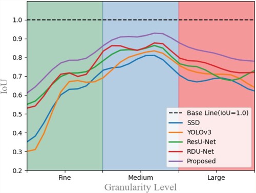
The intersection over Union (IoU) represents the matching performance between a detected target and the ground truth. It is obtained by calculating the ratio of the intersection and union of the detection box and labelled box. Besides, it also indicates the detection ability of comparison methods at each granularity level. We counted the average IoU of each method at different granularity levels. The results are shown in Figure 13. All the comparison methods show a poor detection ability at the fine level and large level. For a small target with low distinguishability at the fine level, methods may miss it then achieve an IoU=0. Meanwhile, the methods may mistakenly detect an overexposed spot as an independent target. Benefit from the proposed enhancement layer, our method demonstrates superiority over others.

Figure 13. Average IoU of comparison methods.

Since there is only one category, i.e. coal, in our task, we modify the definition of mean average precision (mAP): If the IoU of the detection box and the ground truth exceeds 75$\mathrm{\%}$, the result is classified as correct. Otherwise, it is classified as incorrect. The experimental results are given in Table 3. We can see that the proposed method achieves competitive results of average detecting time (Avg.Det.Time) and average training time(Avg.Tra.Time), while in terms of mAP, our method is better than others. Since the proposed enhancement layer can be transplanted as the first layer of any deep network, we further test if the proposed layer could improve the detection performance for other methods. The results are marked as mAP${}^{+}$ in Table 3.

Table 3. Results of speed and mAP on T-DB.

Method	Avg.Tra.Time/h	Avg.Det.Time/ms	mAP/$\mathrm{\%}$	mAP${}^{+}/\mathrm{\%}$
YOLOv3	67.2	147	74.5	77.2
SSD	73.7	119	71.2	75.6
RDU-Net	45.5	172	82.6	85.1
ResU-Net	43.6	98	80.4	82.7
Proposed	50.4	125	84.7	88.7

We investigated the reasons for this as follows. First, we replace the backbone, namely, VGG16, with ResNet101 in the traditional SSD framework. Hence, the proposed method takes advantage of the residual structure and benefits from a deeper network in the feature extraction stage. Second, it is challenging to segment the blocky coal into independent and complete individuals, but our image enhancement method minimises the effects of dust, overexposed spots et al. by improving the coal distinguishability.

The coal detection and granularity estimation task is very different from the targets for the existing detection methods. Therefore, we define an indicator named estimation bias EB to evaluate the performance of comparison methods in granularity estimation. (19) $EB=\sum _{s\in \{fine,medium,large\}}\left(|PGL\right(s)-GT(s\left)|\right),$(19) where $PGL(\bullet )$ and $GT(\bullet )$ refer to as proportions of different granularity levels in detection results and the ground truth, respectively. EB represents the cumulative deviation between the estimated granularity of methods and the ground truth. From the results shown in Table 4, the proposed method achieves the minimum EB of 7.6, illustrating that it is more in line with the actual granularity. Especially for the fine granularity level, our results are more reliable than other comparison methods. It is primarily due to our image enhancement method making objects in an image more distinguishable.

Table 4. Comparison results of coal granularity estimation on T-DB.

	Proportions of different granularity levels /$\mathrm{\%}$
Method	Fine level	Medium level	Large level	Estimation bias /$\mathrm{\%}$
Ground-Truth	38.5	34.1	27.4	–
YOLOv3	50.1	27.5	22.4	23.2
SSD	51.4	56.8	21.8	25.8
RDU-Net	45.6	29.9	24.5	14.2
ResU-Net	44.1	30.8	25.1	11.2
Proposed	42.3	31.8	25.9	7.6

From Table 4, we can see that the proportions of fine granularity level, which is estimated by all methods, are bigger than that of ground truth. In comparison, the proportions of other granularity levels are less than it. Considering the discussion in Section 1, coal detection is challenging due to four main reasons. Therefore, methods may miss rather than mistakenly detect many objects in the detection procedure. However, the proposed method improves the distinguishability of coal in the image, making the detection results more accurate.

We also divide the data set into different proportions for training and testing. The results show that if the training samples are less than 30$\mathrm{\%}$, all the methods appear overfitting. This phenomenon is indicated by the fact that methods achieve an excellent detection performance on the validation set(some methods even achieved AP = 1.0). But in the testing set, all the methods gain an AP lower than 0.5. In this condition, we believe that the models do not learn the commonness of the same target but learn too much about the features that belong to part of the samples. On the contrary, if the proportion of the training set exceeds 70$\mathrm{\%}$, the experimental results tend to be stable and reliable. In terms of the indicator $\mathit{E}\mathit{B}$, YOLOv3 has the most significant difference. When the training set accounts for 90$\mathrm{\%}$, YOLOv3 achieves the best $\mathit{E}\mathit{B}\mathit{=}\mathit{21.8}\mathit{\%}$, while commits the worst $\mathit{E}\mathit{B}\mathit{=}\mathit{24.4}\mathit{\%}$ if the proportion accounts for 75$\mathrm{\%}$. The differences of $\mathit{E}\mathit{B}$ for other methods are no more than 2$\mathrm{\%}$.

6. Conclusion and discussion

In this paper, we proposed an effective method for robust coal granularity estimation. We first analysed the differences between coal detection and other similar tasks and summarised the reasons. Then, we designed a deep neural network structure called Res-SSD, in which the backbone VGG16 replaced with a deeper structure, i.e. ResNet101. To improve the detection performance further, we proposed an image enhancement layer including a series of image enhancement methods, by which the dust can be removed, and the distinguishability of coal can be improved significantly. More specifically, the image denoising method based on dust modelling could suppress the influence of dust. OBT algorithm could remove the overexposed spots brought about by specular reflection. Meanwhile, the OBT could also balance the optical distribution in dark zones.

We have conducted experiments on a large-scale coal database for real scene collection. The comparative study has demonstrated the effectiveness of the proposed method over existing deep network based methods. Thus we conclude that the proposed method is applicable to granularity estimation of coal and provides a novel solution to update the current way. We have tracked the feedback of the proposed method in the practical application for about 12 months and continued to test a total of 50,000 images. The results showed that the accuracy did not decline during this period. However, we should point out that if the coal quality or detection environment changes, the model needs to be retrained by collecting new and sufficient samples.

In the future, our method may also serve as extended to other intelligence scenarios in the coal industry or other object detection tasks in a harsh environment, for example, underground coal-gangue identification and deep-sea target recognition.

Disclosure statement

No potential conflict of interest was reported by the authors.

Correction Statement

This article has been republished with minor changes. These changes do not impact the academic content of the article.

References

- Allegra, R. J., Hawley, A. S., & Holton, G. (1972). Attenuation of sound in suspensions and emulsions: Theory and experiments. The Journal of the Acoustical Society of America, Part 2, 51(1A), 1545–1564. https://doi.org/10.1121/1.1912999
- Amankwah, A., & Aldrich, C. (2011). Automatic ore image segmentation using mean shift and watershed transform. In Proceedings of 21st International Conference Radioelektronika 2011 (pp. 1–4). IEEE.
- Bai, F., Fan, M., Yang, H., & Dong, L. (2021). Image segmentation method for coal particle size distribution analysis. Particuology, 56(6), 163–170. https://doi.org/10.1016/j.partic.2020.10.002
- Belov, G., Boland, N. L., Savelsbergh, M. W., & Stuckey, P. J. (2020). Logistics optimization for a coal supply chain. Journal of Heuristics, 26(2), 269–300. https://doi.org/10.1007/s10732-019-09435-8
- Chen, Y., & Zhang, H. (2020). An improved CV model and application to the coal rock mesocrack images. Geofluids, 4, 1–11. https://doi.org/10.1155/2020/8852209
- Duan, J., Liu, X., & Wu, X. (2020). Detection and segmentation of iron ore green pellets in images using lightweight U-net deep learning network. Neural Computing and Applications, 32(10), 5775–5790. https://doi.org/10.1007/s00521-019-04045-8
- Farid, H. (2001). Blind inverse gamma correction. IEEE Transactions on Image Processing, 10(10), 1428–1433. https://doi.org/10.1109/83.951529
- Gui, H., Xu, J., & Zhang, Y. (2021). Effects of granularity and clay content on the permeability of the fault core in the Renlou coal mine in China: Implications for underground water inrush. Arabian Journal of Geosciences, 14(4), 1–18. https://doi.org/10.1007/s12517-021-06645-y
- He, K., Zhang, X., Ren, S., & Sun, J. (2016). Deep residual learning for image recognition. In Proceedings of the IEEE Conference on Computer Vision and Pattern Recognition (pp. 770–778). IEEE.
- He, M., & Tang, X. (2010). Single image haze removal using dark channel prior. IEEE Transactions on Pattern Analysis and Machine Intelligence, 33(12), 2341–2353. https://doi.org/10.1109/TPAMI.2010.168
- He, M., & Tang, X. (2012). Guided image filtering. IEEE Transactions on Pattern Analysis and Machine Intelligence, 35(6), 1397–1409. https://doi.org/10.1109/TPAMI.2012.213
- Hu, X. Y., & Nikolaus, K. J. (2017). Using settling velocity to investigate the patterns of sediment transport and deposition. Acta Pedologica Sinica, 54(5), 1115–1124. https://doi.org/10.11766/trxb201703100056
- Jiang, D., Qu, H., Zhao, J., Zhao, J., & Hsieh, M. Y. (2021). Aggregating multi-scale contextual features from multiple stages for semantic image segmentation. Connection Science, 33(3), 1–18. https://doi.org/10.1080/09540091.2020.1862059
- Kholerdi, H. A., Taherinejad, N., Ghaderi, R., & Baleghi, Y. (2016). Driver's drowsiness detection using an enhanced image processing technique inspired by the human visual system. Connection Science, 28(1), 27–46. https://doi.org/10.1080/09540091.2015.1130019
- Liu, W., Anguelov, D., Erhan, D., Szegedy, C., Reed, S., Fu, C. Y., & Berg, A. C. (2016). SSD: Single shot multibox detector. In European Conference on Computer Vision (pp. 21–37). Springer.
- Liu, X., Zhang, Y., & Jing, H. (2020). Ore image segmentation method using U-Net and Res-Unet convolutional networks. RSC Advances, 10(16), 9396–9406. https://doi.org/10.1039/C9RA05877J
- Luo, Y. X., Lin, F. L., & Jiang, H. Z. (2013). Ore particle size online detecting system based on image processing. Instrument Technique and Sensor, 7(3), 63–66. https://doi.org/10.3969/j.issn.1002-1841.2015.07.020
- Nader, J., Alqadi, Z. A., & Zahran, B. (2017). Analysis of color image filtering methods. International Journal of Computer Applications, 174(8), 12–17. https://doi.org/10.5120/ijca2017915449
- Purswani, P., T. Z Karpyn, & Enab, K. (2020). Evaluation of image segmentation techniques for image-based rock property estimation. Journal of Petroleum Science and Engineering, 195, 107890. https://doi.org/10.1016/j.petrol.2020.107890
- Redmon, J., & Farhadi, A. (2018). YOLOv3: An incremental improvement. arXiv e-prints.
- Rubey, W. W. (1933). Settling velocity of gravel, sand, and silt particles. American Journal of Science, 25(148), 325–338. https://doi.org/10.2475/ajs.s5-25.148.325
- Sengupta, A., Ye, Y., Wang, R., Liu, C., & Roy, K. (2019). Going deeper in spiking neural networks: VGG and residual architectures. Frontiers in Neuroscience, 13, 95. https://doi.org/10.3389/fnins.2019.00095
- Sun, J., Zhi, G., & Hitzenberger, R. (2017). Emission factors and light absorption properties of brown carbon from household coal combustion in China. Atmospheric Chemistry and Physics, 17(7), 4769–4780. https://doi.org/10.5194/acp-17-4769-2017
- Sun, X., Wang, Q., Zhang, X., Xu, C., & Zhang, W. (2021). Deep blur detection network with boundary-aware multi-scale features. Connection Science, 1–19. https://doi.org/10.1080/09540091.2021.1933906
- Tang, K., Astola, J., & Neuvo, Y. (1995). Nonlinear multivariate image filtering techniques. IEEE Transactions on Image Processing, 4(6), 788–798. https://doi.org/10.1109/83.388080
- Wang, W., Li, Q., & Xiao, C. (2021). An improved boundary-aware U-Net for ore image semantic segmentation. Sensors, 21(8), 2615. https://doi.org/10.3390/s21082615
- Wei, Z., & Jiang, D. (2011). The marker-based watershed segmentation algorithm of ore image. In Communication Software and Networks, IEEE 3rd International Conference (Vol. 472, pp. 27–29). IEEE.
- Wu, Z., Gao, Y., Li, L., Xue, J., & Li, Y. (2019). Semantic segmentation of high-resolution remote sensing images using fully convolutional network with adaptive threshold. Connection Science, 31(2), 169–184. https://doi.org/10.1080/09540091.2018.1510902
- Xiao, D., Liu, X., Le, B. T., Ji, Z., & Sun, X. (2020). An ore image segmentation method based on RDU-Net model. Sensors, 20(17), 4979. https://doi.org/10.3390/s20174979
- Xu, Z., & Zhang, W. (2020). Hand segmentation pipeline from depth map: An integrated approach of histogram threshold selection and shallow CNN classification. Connection Science, 32(2), 162–173. https://doi.org/10.1080/09540091.2019.1670621
- Yang, H., Huang, C., Wang, L., & Luo, X. (2021). An improved encoder–decoder network for ore image segmentation. IEEE Sensors Journal, 21(10), 11469–11475. https://doi.org/10.1109/JSEN.2020.301-6458
- Yang, Z., Huang, J., & Wang, Z. (2019). Unique advantages of gasification-coke prepared with low-rank coal blends via reasonable granularity control. Energy & Fuels, 33(3), 2115–2121. https://doi.org/10.1021/acs.energyfuels.8b04504
- Ye, K. P. (2018). Research on ore and rock particle size detection based on image processing [Doctoral dissertation].
- Zhan, Y., & Zhang, G. (2019). An improved OTSU algorithm using histogram accumulation moment for ore segmentation. Symmetry, 11(3), 431. https://doi.org/10.3390/sym11030431
- Zhang, G., Liu, G., & Zhu, H. (2011). Segmentation algorithm of complex ore images based on templates transformation and reconstruction. International Journal of Minerals, Metallurgy, and Materials, 18(4), 385–389. https://doi.org/10.1007/s12613-011-0451-8
- Zhang, N., & Deng, J. (2019). Influence of granularity on thermal behaviour in the process of lignite spontaneous combustion. Journal of Thermal Analysis and Calorimetry, 135(4), 2247–2255. https://doi.org/10.1007/s10973-018-7440-3
- Zhang, Z., Liu, Y., Hu, Q., Zhang, Z., Wang, L., Liu, X., & Xia, X. (2020). Multi-information online detection of coal quality based on machine vision. Powder Technology, 374, 250–262. https://doi.org/10.1016/j.powtec.2020.07.040
- Zhang, Z., Yang, J., & Ding, L. (2012). Estimation of coal particle size distribution by image segmentation. International Journal of Mining Ence and Technology, 5, 739–744. https://doi.org/10.1016/j.ijmst.2012.08.026
- Zhang, Z., Yang, J., & Su, X. (2013). Analysis of large particle sizes using a machine vision system. Physicochemical Problems of Mineral Processing, 49(2), 397–405. https://doi.org/10.5277/ppmp130202
- Zhou, Y., & Hui, R. (2012). Segmentation method for rock particles image based on improved watershed algorithm. In 2012 International Conference on Computer Science and Service System (pp. 347–349). IEEE.
- Zhu, Q., Mai, J., & Shao, L. (2015). A fast single image haze removal algorithm using color attenuation prior. IEEE Transactions on Image Processing, 24(11), 3522–3533. https://doi.org/10.1109/TIP.2015.2446191
- Zhu, X., Zuo, J., & Ren, H. (2020). A modified deep neural network enables identification of foliage under complex background. Connection Science, 32(1), 1–15. https://doi.org/10.1080/09540091.2019.1609420
- Zou, F., Shen, L., Jie, Z., Zhang, W., & Liu, W. (2019). A sufficient condition for convergences of adam and rmsprop. In Proceedings of the IEEE/CVF Conference on Computer Vision and Pattern Recognition (pp. 11127–11135). IEEE.