Automatic classification method of liver ultrasound standard plane images using pre-trained convolutional neural network

Abstract

The liver ultrasound standard planes (LUSP) have significant diagnostic significance during ultrasonic liver diagnosis. However, the location and acquisition of LUSP could be a time-consuming and complicated mission and requires the relevant operator to have comprehensive knowledge of ultrasound diagnosis. Therefore, this study puts forward an automatic classification approach for eight types of LUSP based on a pre-trained CNN(Convolutional Neural Network). With the comparison to classification methods on the basis of conventional hand-craft characteristics, the method proposed by us can automatically catch the appearance in LUSP and classify the LUSP. The proposed model is consisted of 13 convolutional layers with little 3×3 size kernels and three completely connected layers. To address the limitation of data, we adopt the transfer learning strategy, which pre-trains the weight of convolutional layers and fine-tune the weight of fully connected layers. These extensive experiments show that the accuracy of the suggested method reaches 92.31%, as well as the performance of the suggested means outperforms previous ways, which demonstrates the suitability and effectiveness of CNN to classify LUSP for clinical diagnosis.

KEYWORDS:

• Ultrasound images
• liver standard plane
• image classification
• convolutional neural network

1. Introduction

Assessment of liver healthy through ultrasound imaging is used worldwide in clinical liver examination because of its non-invasive and practicability (Spencer & Adler, 2008). In general, the clinical liver examination is divided into manual scanning, positioning of the liver ultrasound standard plane (LUSP) and diagnosis (Sidhu, 2005). Especially, searching for LUSP is of great significance because LUSP can clearly describe the anatomy of the liver and contribute to liver disease diagnosis (Carneiro et al., 2008a; Chen et al., 2016; Dudley & Chapman, 2002; Salomon et al., 2006; Wu et al., 2017; Zhang et al., 2012). However, the task of searching LUSP could not only be time-consuming and laborious. In addition, it also requires the relevant operator to have sufficient knowledge and practical experience (Crino et al., 2010; Kwitt et al., 2013). Therefore, this task is challenging for novice and even difficult for expert physicians to complete it quickly. So, an automatic classification approach for LUSP is strongly demanded in clinical practice to improve examination efficiency (Ni et al., 2013).

In this work, we researched the classification algorithm for LSUP from 2D ultrasound images. Specifically, eight LUSP: (1) Hepatic Vein (HV):; 2) Inferior Vena Cava (IVC); 3) First Porta Hepatis (FPH); 4) Second Porta Hepatis (SPH); 5) Transabdominal Aorta (AA); 6) Liver Right Kidney (LRK); 7) Liver-Gallbladder (LG); and 8) Left Liver Lobe (LLL) are shown in Figure 1. In the HV, the hepatic vein is visible. From IVC, we can see the inferior vena cava. FPH show the short axis of the main portal vein, and thick left and right branches are displayed on the right side of the hepatic portal groove. SPH show the proximal end of the hepatic vein. AA shows a longitudinal section of the left outer lobe of the liver. LRK show a portal vein branch inside the right lobe of the liver. The definition of LG is mainly the right liver short-axis cross-section of the anterior lobe. LLL show left liver lobe. These eight LUSP completely cover the entire liver, which helps the doctor observe the liver and diagnose.

Figure 1. The [a2]-[h2] represents the example of the eight categories of LUSP with the feature of each category in the yellow box: (a2) HV: the hepatic vein are visible, (b2) IVC: In this view, we can see the inferior vena cava, (c2) FPH show the short axis of the dominant portal vein and the thick left and right branches are displayed on the right side of the hepatic portal groove, (d2) SPH show the proximal end of the hepatic vein, (e2) AA show longitudinal section of left outer lobe of the liver, (f2) LRK show portal vein branch inside the right lobe of the liver, (g2) LG show the right liver short-axis cross-section of the anterior lobe, (h2) LLL show left liver lobe.

However, it is a challenging research, on the one hand, because the LUSP images have intrinsic bad characteristics, such as shadow and speckle noise caused by the imaging principle of an ultrasonic machine. In this case, massed research papers have been put forward in previous decades (Lei et al., 2015a,2015b; Rahmatullah & Noble, 2014; Shi et al., 2016) to address these issues. These methods in these papers are mainly about conventional machine learning and deep learning. Among, conventional machine learning techniques need to manually design relevant characteristics, such as Histogram of Oriented Gradients that is also known as HOG (Dalal & Triggs, 2005), Local Binary Patterns (LBP) (Wang et al., 2010). In contrast, deep learning models can automatically access the relevant features from numerous training data. Usually, in the ultrasound image process field, the performance result of methods on the basis of deep learning better than methods based on conventional machine learning techniques because the ultrasound images are hard to manually design effective features (Carneiro et al., 2008b). On the other hand, deep learning models are difficult to apply on ultrasound image data, because of the limited availability of large ultrasound images. Regarding this problem, there are two mitigation methods. The approaches could be separated into two types: the first could be to increase data volume via data augmentation (Wong et al., 2016). Traditional data augmentations must be geometric transformations, for example, flipping, cropping, etc, as well as transformations of colour (Fawzi et al., 2016). Meanwhile, Generative Adversarial Net (GAN)n has been proved to be an effective data augmentation method by synthesising images (Bowles et al., 2018; Wu et al., 2018; Wu et al., 2020). Furthermore, another solution is the transfer learning strategy which reduces the amount of data required for network training by transferring large data set knowledge to the medical image.

We proposed a 13 layers CNN model to classify LUSP. In this model, we choose small size kernel to catch the distinguishing intra-class features. What's more, we applied the way of transferring learning to undertake the process of training the model for us, which avoided overfitting the model. As the largest range we could get, it could be the initial LUSP classifier, and our result could express that the suggested means has the capacity to accomplish this task well.

The following part from Sections 2–5. Section 2 illustrates various relevant works. Section 3 explores the methodology of the suggested means. Experimental setup, as well as results, have been shown in Section4, Section 5 makes a conclusion of the task.

2. Related work

Transfer learning (TL) could be a training strategy in deep learning. This method is mainly to apply the pre-trained weights trained by large cross-domain datasets to initialise the new network. In this way, over-fitting caused by a lack of data can be effectively alleviated, and network training can be accelerated (Shin et al., 2016). Transfer learning is widely applied in many different fields (Cao et al., 2021; Greenspan et al., 2016; Litjens et al., 2017; Shen et al., 2017), especially in medical image process applications, because the medical images are hard to collect and the limited amount of data makes it difficult to train a large deep learning network. However, by transfer learning, we can transfer the weight parameters of the network trained under the large data set to the new network, and then we only need to train the full connection layer of the network (Kajbakhsh et al., 2016a). By this way, the issue directed by the small amount of data could be effectively alleviated (Kajbakhsh et al., 2016a; Sato et al., 2018).

Many works proposed to search for standard fetal planes. The aim of those works is to detect standard fetal plane (Carneiro et al., 2008b; Lu et al., 2008; Rahmatullah et al., 2011; Yu et al., 2008). Some works are based on ultrasound videos, such as Zhang et al. (2012) proposed an intelligent scanning system, which can automatically locate the standard plane. This method is on the basis of cascaded AdaBoost classifiers as well as information of local context. This work was validated on 31 ultrasound videos, and the effect of the suggested system was close to the effect of the radiologist. Some works based on Rahmatullah et al. (2012) proposed a semi-automatic identification means for observing anatomical formations by manually extracting global and local features of ultrasound images. This approach was applied in 2348 2D ultrasound images, and the result shows that it can outperform related works based on local-global features. However, both of the above examples are based on conventional hand-craft features, making the method less generalised. Except for some 2D image processing, there are also some new ideas for 3D image processing. In terms of 3D graphics, Cai et al. (2021) put forward a parallel neural network on the foundation of three-dimensional voxels, which showed good performance compared with traditional neural networks based on simple spatial location information. This undoubtedly provides a new idea for medical 3D image recognition and segmentation. Wang et al. (2021) introduced some recent representative methods of deep learning, which are used in 3D vision applications. For the application of deep learning methods to 3D views, Qi et al. (2021) introduced many deep learning means for multi-view 3D object recognition exactly.

Motivated by the development of computer vision and computing power, there has been proposed some works based on CNN. Bai et al. (2021) have made relevant review studies on the interpretation of deep learning and have made in-depth discussions on the compression and acceleration of convolutional neural networks, robustness and other issues. The application deployment of deep learning has been greatly promoted. There is also some related work based on CNN. Chen et al. (2017) expressed one means on the foundation of learning on the foundation of the domain transferred CNN to place the fetal abdominal standard plane in ultrasound video. This work achieved better performance than previous work because the CNN can represent the complicated appearance on the standard plane. Meanwhile, this work demonstrated that transfer learning is an effective solution for insufficient training samples in the medical image process. However, CNN is more suitable for processing images data than video sequence data. Thus, Chen et al. (2015) carried out a classification completely to fetal ultrasound standard plane on the field of ultrasound video sequences in an automatic way. This main work contribution was proposing a brand-new composite structure of CNN and RNN which can explore in-and between-plane feature learning and further locates the item of training data with limitation. Finally, the experiment results in locating standard plane get up to 90%and demonstrated it is an effective and general framework. The disadvantage of the work is that the composite neural network ought to be utilised several times. It could preclude relevant systems from operation in real-time. Yu et al. (2018) put forward the automatic sort way of the standard plane of fetal facial ultrasound images, and they also use neural network structure. Here, the author proposed a novel global average pooling. Concerning this, the function could decrease the network parameters to achieve the purpose of alleviating the overfitting problems and improving the performance. Under this method, the cognition rate of the standard plane is getting up to 95%and the model can improve performance in real-time. At the same time, CNN is also widely used in feature extraction. Ning et al. (2021) put forward a feature enhancement means on the foundation of the RES-50 skeleton for human recognition. Weakening factors are used to weaken the features extracted by CNN to highlight the important role of global features in recognition. Moreover, a multi-branch attention network is used to obtain more valuable features driven by weakening factors for feature extraction. Srivastava and Biswas (2019) used the feature extraction capabilities of CNN to obtain the information features of the benchmark hyperspectral Images (HSI) datasets from different CNN models. The combination of depth features and spectral features increases the information knowledge in the image database. In addition to being used for feature extraction, CNN is also utilised for image classification; Ying et al. (2021) combine the advantages of CNN in image processing to provide a useful method for improving the effectiveness of crime scene investigation image classification.

3. Methodology

3.1. Data and task definition

The dominant task of this study could be to develop an automatic classification algorithm for eight LUSP. Retrospective ultrasound data were acquired from the collaborating hospital, post appropriate ethical clearance. The research data were obtained from subjects in JPG format. Depending on the machine parameters, the dimensions of data obtained were either 695×588 or 787×514. The research data in this paper includes eight categories of LUSP, the names of the eight standard planes are as follows: Hepatic Vein (HV), Inferior Vena Cava (IVC), Liver Right Kidney (LRK), Liver-Gallbladder (LG), and Left Liver Lobe (LLL), First Porta Hepatis (FPH), Second Porta Hepatis (SPH), Transabdominal Aorta (AA). Figure 1 could reflect an image case of different types. Besides, the annotations of the acquired data were reviewed by an expert with experience of about ten years and the research protocol was checked and obtained approval by the official from the overall subjects.

3.2. Overview

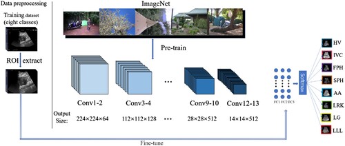
The method overview is shown in Figure 4. Since the ultrasound images have some character or Kepler colour map, which will have a bad influenced on performance of the method. In order to address the problem, we firstly preprocessed the input images. In particular, the pre-process method has low computational complexity, so it will not affect the model performance. Then we apply the ImageNet dataset to pretrain the model. After that, follow the two steps below: 1) keep the convolutional layers frozen, 2) fine-tune the full connected layer using the LUSP dataset.

3.2.1. Data preprocessing

The first step is ROI area extraction. The main task of this step is to eliminate non-primary features and perfect the learning efficiency concerning the network. The means could be divided into 3 steps: 1) image binarization. This step aims to enhance the contrast to distinguish between the liver region and non-liver region. As shown in Figure 2, the liver area is white and black is the background. 2) image open operation. The main purpose of this step is to eliminate non-liver regions that are misjudged as liver regions. 3) liver region location. After the above two steps, the white areas all represent the liver area. Thus, the goal of this process is to get the white area and to generate a new image, which only contains the liver regions. Meanwhile, we demonstrate the robustness of the means by testing ultrasound images from many ultrasonic machines. The test result is shown in Figure 3. From the result, we can see that the means could be fit for all liver ultrasound images.

Figure 2. The flow chart of the pre-processing method.

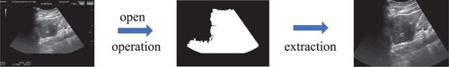
Figure 3. Test results of ROI extraction method on the ultrasound images from the different ultrasound machines. (A1)–(A3): original images, (B1)–(B3): the result of the open operation, (C1)–(C3): the final ROI result.

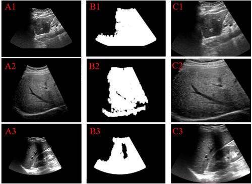
Image reshape and normalisation. The images have dimensions of either 695×588 or 787×514. However, the input size of the model is fixed. Thus, we reshape all images into 224×224. Besides, the image data was further normalised to have intensity values between zero and one using Eq. 1, wherein min (img) and max (img) represents the minimum as well as maximum values of the pixel intensities in an ultrasound image. (1) $\begin{array}{r}Normalized\mathrm{\_}img=\frac{img-min(img)}{max(img)-min(img)}\end{array}$(1)

3.3. Neural network architecture

Convolutional Neural Network, which is short for CNN. The invention of CNN was inspired by the human neural system. In recently years, CNN has got significant achievements in many sides, including object detection, cognition and classification and so on, because CNN has a powerful capability to learn nonlinear and abstract feature map from training datasets (Razavian et al., 2015).

The basic architecture of CNN contains convolutional layers, subsampling layers and fully connected layers (Nagi et al., 2011). The goal of the convolution layers must collect different features by a convolution kernel. The shallow layers of the convolutional network are mainly used to extract shallow features such as image edges, image sizes, etc. The depth feature is obtained by iterating over multiple convolution layers. Suppose that $f_j^l$ is the $\text{j}$th characteristic’s map in the $l$th layer and $f_m^{l-1}$ ($m=1,2,3,\dots .,M)$ is the $m$th characteristic map in the $(l-1)th$ layer, the characteristic map $f_j^l$ could be calculated by: (Rahmatullah et al., 2011) (2) $\begin{array}{r}{f}_j^l=\sigma ({\sum }_{m=1}^M{W}_{jm}^l\times f_m^{l-1}+b^l)\end{array}$(2) where $W_{jm}^l$ is the weight parameter; $b^l$ could be the bias in the $l$th layer; and $\sigma (.)$. In terms of this point, it could represent the function of nonlinear activation. In our implementation, rectified linear unit (ReLU) is employed as the activation function as its function of accelerating network convergence and preventing gradients from disappearing. Besides, the Relu function can get better results compared with the traditional sigmoid function.

The pooling layer could be utilised to cut the resolution of the characteristic map as well as decrease the parameters of the network. In our study, max-pooling is used as a pooling layer. Max pooling plays a vital role in convolutional neural networks. It is often used to decrease the dimensionality of features, compress the number of data and parameters, and also prevent overfitting. You et al. (2021) have proposed a deep convolutional network model with some max-pooling modules, which is used for medical image pixel segmentation and obtained very good results. The completely connected layer is usually the last layer of the CNN structure, and it is used to classify the feature map extracted by convolution layers. The ultimate layer of the CNN is used to get the possibility of each class with the softmax function.

Simonyan & Zisserman, 2014 proposed CNN. In this paper, the pre-trained VGG16 CNN is applied in our experiment. Table 1 shows the network structure of VGG16. VGG16 contains 13 layers of convolutional layers and 3 layers of completely connected layers. The size of the input images is set as 224 × 224. The convolution kernel size is defined as 3 × 3, because little Conv kernel size can reduce the amount of parameters. What's more, Convolution layer with little Conv kernel size can extract subtle features and the depth of the network can be deeper than large Conv kernel size.

Table 1. Detail configuration of VGG-16.

Layer	Kernel size	Output size
Conv1-2	3×3	224×224×64
Max-Pool2	2×2	112×112×64
Conv3-4	3×3	112×112×128
Max-Pool	2×2	56×56×128
Conv5-7	3×3	56×56×256
Max-Pool	2×2	28×28×256
Conv8-10	3×3	28×28×512
Max-Pool	2×2	14×14×512
Conv11-13	3×3	14×14×512
Max-Pool	2×2	7×7×512
FC1		1×1×4096
FC2		1×1×4096
FC3		1×1×8
	Softmax

3.4. Training

The proposed model was trained in Linux 16.04 system. The input image of the network is set as 224 × 224, the batch size is set as 25, the learning rate is set as 0.0001. In the process of training, we first imported the weights trained by ImageNet as the initial weights of the network, and then locked the weights of the hidden layer except for the complete connection layer. We only retrained the full connection layer and changed the production of the complete connection layer to 8, because the task of the network is eight classification tasks.

Besides, the training optimiser is set as Adam (Kingma & Ba, 2014). Adam is currently the most popular optimisation method. It can update the weights of neural networks based on training data iteratively, which is different from traditional stochastic gradient descent, which is short for SGD. SGD maintains the same learning rate throughout the training process, while Adam updates the learning rate based on changes in the gradient during each iteration. In the deep learning field, Adam is suitable for the neural network. The main reason comes to that it could obtain better results quickly. Empirical results could express that the Adam algorithm has a superior manifestation in practice. In addition, it has excellent merits over other random optimisation algorithms. Among them, the decay formula of learning rate is shown in Eq. 3 (3) $\begin{array}{r}{\alpha }_t=\alpha \cdot \sqrt{1-{\beta }_2^t}/(1-{\beta }_1^t)\end{array}$(3) In Eq. 3, $\alpha$ represents the learning rate, ${\alpha }_t$ represents the learning rate after decay. ${\beta }_2^t$, ${\beta }_1^t$ represents exponential decay rates. And ${\beta }_2^t$, ${\beta }_1^t\in$ [0,1]. In the training processing, we initially set $\alpha$=0.0001, ${\beta }_1^t$=0.9, ${\beta }_2^t$=0.999.

Concerning loss calculation, the cross-entropy loss has been selected to compute the loss. Generally, the cross-entropy loss function has obvious classification effectiveness in a multi-classification assignment. Categorical loss is shown as Eq. 4. (4) $\begin{array}{r}Loss={\sum }_{i=1}^N-[y^i\log {\hat{y}}^i+(1-y^i)\log (1-y^i)]\end{array}$(4) In Eq. 4, N could stand for the number of class, i stands for the current category. y represents the ground truth, $\hat{y}$ represents the prediction result. As you can see from the formula, as y and $\hat{y}$ get closer and closer, the loss will be lower and lower, which meets the classification task requirement. In summary, we can see that the overall neural network framework is shown in Figure 4. The CNN initially load pre-trained weight parameters using the ImageNet dataset, then fine-tune the weight parameter of fully connected layers with our liver ultrasound images dataset. Finally, the model output the class of the input images.

Figure 4. Overview of the proposed classification method.

4. Results and analysis

4.1. Experimental setup

1. LUSP dataset: The research data of this paper is mainly provided by the Second Affiliated Hospital of Fujian Medical University. Supersonic explorer, GE Voluson E8 and GE Voluson E10 are used in sampling ultrasound images. The patient age range is 10–60, including male and female, normal and diseased. The overall data is currently 4682, and the number of each category is HV (653), IVC (592), FPH (637), SPH (569), AA (1728),LRK (932), LG (815), LLL (863).

2. Experimental equipment: This experiment implemented the model using Keras (version: 2.1.0) and Tensorflow. The code is implemented in the ubuntu16.04 system, and the experimental computer is equipped with a GPU (Nvidia GTX1060).

4.2. Evaluations of model

1. Evaluation indicators:

With the goal to assess the quality of the model, macro precision rate (macro-P), macro recall rate (macro-R), and specificity (macro-Sp) are introduced. The formulas of evaluation indicators are as follows. (5) $\begin{array}{rl}macro-P& =\frac{1}{n}\sum _{i=1}^n{P}_i\end{array}$(5) (6) $\begin{array}{rl}macro-R& =\frac{1}{n}\sum _{i=1}^n{R}_i\end{array}$(6) (7) $\begin{array}{rl}macro-Sp& =\frac{1}{n}\sum _{i=1}^{n}S{p}_i\end{array}$(7)

In the formula (5), then expresses the amount of class, i stands for the i_th class, the P_i represents the precision in i_th class. Meanwhile, in the formula (6), the R_i represents the recall in i_th class. Macro-Sp is calculated by the formula (7), the Sp_i represents the specificity in i_th class. Besides, formula (8), (9), (10) shows how Pi, Ri and Spi is counted. Meanwhile, TP is the abbreviation of true positives, FP is the abbreviation of false positives, TN is the abbreviation of true negatives, as well as FN is the abbreviation of false negatives. (8) $\begin{array}{rl}{P}_i& =\frac{TP}{TP+FP}\end{array}$(8) (9) $\begin{array}{rl}{R}_{\text{i}}& =\frac{TP}{TP+FN}\end{array}$(9) (10) $\begin{array}{rl}Sp& =\frac{TN}{TN+FP}\end{array}$(10)

1. Evaluation of Model training and classification

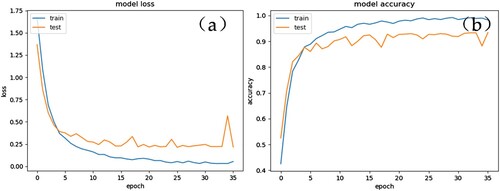
With the goal to demonstrate the training process of VGG16 with fine-tuning on the ImageNet, the loss curve and accuracy curve was described and shown in Figure 5. Early-Stopping training strategy in Keras was applied in the training process. This strategy improves network training efficiency by monitoring loss value during training. Under the situation that the loss value could not be cut within p epochs, the relevant network will stop training. In this experiment, the p is set as 10. From Figure 5, we can see that the network converges after 35 epochs, and the minimum value of the loss reaches 0.2456 in 25 epochs, and the network stops training after 10 epochs.

Figure 5. The loss cure and accuracy curve of fine-tuning of the proposed CNN model: (a) Validation loss curve, and (b) training curve for VGG16 that fine-tuning all network layers with ImageNet pre-trained models.

To demonstrate the advantages of the DCNN for LUSP classification, we will use accuracy, macro-P, etc to check the model classification effect. The metrics’ evaluation results have been expressed in Table 3. We can see that the classification results of our model for eight different LUSP. HV, IVC, AA, LRK and LG are well classified, and their classification accuracy reaches over 90%. However, there are also some categories that don't perform so well, such as FPH, SPH, and LLL. In order to show the experimental results better, the confusion matrix and ROC curve have also been shown in Figure 6, from which we can better intuitively see the classification results of each category and the performance of the model in each category.

Figure 6. Feature maps of Conv layers learned by suggested CNN models (VGG16 with pre-trained weight). (a1) - (f1) correspond original images, (a2) - (f2) correspond feature map images.

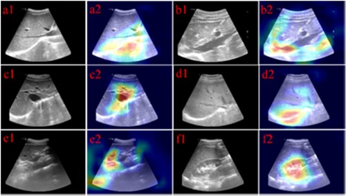
From the data in Table 2, we can see that the classification result of the model in most categories has reached the ideal result, and the total classification accuracy of the model has reached 92.31%, which also indicates that the model can reach the ideal result in the test set.

Table 2. LUSP classification result (%).

Class name	Number	Macro-P	Macro-R	Marco-Sp
HV	167	99.00	78.03	82.34
IVC	156	94.46	92.21	88.35
FPH	131	78.74	83.91	78.44
SPH	129	77.83	80.76	80.32
AA	413	95.95	98.05	96.34
LRK	294	99.6	99.04	99.12
LG	231	97.84	96.11	95.49
LLL	228	83.62	85.13	80.03
Macro-avg		90.88	89.15	86.45

In order to demonstrate that fine-tuning is an effective strategy, we make the comparative experiment, and the algorithm includes CNN with random initialisation (CNN-RI)VS CNN with fine-tuning (CNN-FT)and CNN-FT VS SVM.

Upon comparison, we observe that the AUC in every category has been perfected greatly while training via fine-tuning. Meanwhile, SVM's performance in each category is poor, which means deep learning technology could be appropriate for LUSP classification tasks. Besides, Table 3 also exactly expresses that the result of the SVM is not satisfactory compared with the deep CNN method. Furthermore, the result of CNN-FT is better than CNN-RI, which illustrate that the TL strategy is an effective training method for CNN to perfect the classification's accuracy with limited training data volume. With the goal to demonstrate the performance of the model, we compared the other related system (Yu et al., 2018). The comparison results are shown in the Table 3. The proposed model in the references of Yu Z et al, was designed to classify fetal facial standard planes. From the experimental result, we can see that when the model in ref [35] is applied to classify the LUSP, the performance result is worse than the proposed model.

1. Visualisation of the convolution feature map

Table 3. CNN-FT, CNN-RI and SVM classification result (%).

Classifier name	Macro-P	Macro-R	Macro-Sp	Accuracy
CNN -FT	90.88	89.15	86.45	92.31
CNN -RI	83.40	82.30	81.94	85.40
SVM + LBP + HOG	72.50	74.20	71.56	75.30
Ref[35]	82.84	81.47	80.96	84.56

In order to further understand the convolution kernel, we also drew a heat map of the convolution kernel. The convolution heat map is expressed in Figure 6. The heat map can well show the focus of the convolution kernel. The focus of convolution is the colour area in the heat map. In Figure 6, the key features of each category convolution focus can be seen very intuitively. In the ultrasound image, the gray-scale difference area is the focus of the sonographer, and the results in Figure 6 could reflect that the focus area of the convolution is generally in the area where the gray-scale difference is large. Such as black areas, bright areas. These areas generally refer to blood vessel or organ boundaries. The experimental results could show that CNN has super feature learning ability as well as expressive ability, which can automatically and efficiently get the intra-class features and classify better.

5. Conclusion

We assessed the effectiveness of the suggested LUSP classification method by doing comparative experiments. In medical applications, the most prone problem for DCNN must be the shortage of training datasets that leads to model overfitting and test results degradation. Therefore, in the experiment, we use fine-tuning to alleviate this problem. From the ending data of the comparison experiment, it could be seen that the classification performance of the DCNN with transfer learning strategy is better than the DCNN with randomly initialised and the SVM based on the traditional manual features. This also means that transfer learning is an effective strategy for training powerful DCNN models in medical image processing. Besides, we did additional experiments with the related algorithm. The experimental result shows that our model performs better than related algorithms in LUSP classification.

In this study, we first put forward an automatic LUSP classification model. Meanwhile, the paper made a comparative analysis between the suggested model and algorithms with other classification. The experimental results have expressed that the suggested model can more effectively classify LUSP than other classifiers. The fine-tune strategy can efficaciously relieve the disadvantage of a small datasets to some extent. Therefore, the combination of deep learning and ultrasound liver standard plane classification will have a excellent prospect in clinical application and deserve further exploration and research.

Acknowledgements

This work was supported by the Quanzhou scientific and technological planning projects (No.2018C113R, 2018N072S)

Disclosure statement

No potential conflict of interest was reported by the author(s).

References

- Bai, X., Wang, X., Liu, X., Liu, Q., Song, J., Sebe, N., & Kim, B. (2021). Explainable deep learning for efficient and robust pattern recognition: A survey of recent developments. Pattern Recognition, 120, 108102. https://doi.org/10.1016/j.patcog.2021.108102
- Bowles, C., Chen, L., Guerrero, R., Bentley, P., Gunn, R., Hammers, A., Dickie, D. A., Hernández, M. V., Wardlaw, J., & Rueckert, D. (2018). GAN augmentation: Augmenting training data using generative adversarial networks. arXiv preprint arXiv:1810.10863.
- Cai, W., Liu, D., Ning, X., Wang, C., & Xie, G. (2021). Voxel-based three-view hybrid parallel network for 3D object classification. Displays, 69, 102076. https://doi.org/10.1016/j.displa.2021.102076
- Cao, Z., Zhou, Y., Yang, A., & Peng, S. (2021). Deep transfer learning mechanism for fine-grained cross-domain sentiment classification. Connection Science, 33(4), 911–928. https://doi.org/10.1080/09540091.2021.1912711
- Carneiro, G., Amat, F., Georgescu, B., & Comaniciu, D. (2008a). Semantic Car based indexing of fetal anatomies from 3-D ultrasound data using global/semi-local context and sequential sampling. IEEE Computer society Conference on Computer Vision and Pattern recognition.
- Carneiro, G., Georgescu, B., Good, S., & Comaniciu, D. (2008b). Detection and measurement of fetal anatomies from ultrasound images using a constrained probabilistic boosting tree. IEEE Transactions on Medical Imaging, 27(9), 1342–1355. https://doi.org/10.1109/TMI.2008.928917
- Chen, H., Ni, D., & Qin, J. (2015). Standard plane localization in fetal ultrasound via domain transferred deep neural networks. IEEE Journal of Biomedical and Health Informatic, 19(5), 1627–1636. https://doi.org/10.1109/JBHI.2015.2425041
- Chen, H., Wu, L., & Dou, Q. (2017). Ultrasound standard plane detection using a composite neural network framework. IEEE Transactions on Cybernetics, 47(6), 1576–1586. https://doi.org/10.1109/TCYB.2017.2685080
- Chen, H., Zheng, Y., Park, J. H., Heng, P. A., & Zhou, S. K. (2016). Iterative multi-domain regularized deep learning for anatomical structure detection and segmentation from ultrasound images. In S. Ourselin, L. Joskowicz, M. Sabuncu, G. Unal, & W. Wells (Eds.), Medical image computing and computer-assisted intervention – MICCAI (pp. 487–495). Springer.
- Crino, J., Finberg, H. J., Frieden, F., Kuller, J., Odibo, A., Robichaux, A., Bohm-Velez, M., Pretorius, D. H., Sheth, S., Angtuaco, T. L., & Hamper, U. M. (2010). AIUM practice guideline for the performance of obstetric ultrasound examinations. Journal of Ultrasound in Medicine Official, 29(1), 157–166. https://doi.org/10.7863/jum.2010.29.1.157
- Dalal, N., & Triggs, B. (2005). Histograms of oriented gradients for human detection. International Conference on Computer Vision & Pattern Recognition (CVPR ‘05).
- Dudley, N. J., & Chapman, E. (2002). The importance of quality management in fetal measurement. Ultrasound in Obstetrics and Gynecology, 19(2), 190–196. https://doi.org/10.1046/j.0960-7692.2001.00549.x
- Fawzi, A., Samulowitz, H., Turaga, D., & Frossard, P. (2016). Adaptive data augmentation for image classification. IEEE International Conference on image processing (ICIP), 3688-3692.
- Greenspan, H., van Ginneken, B., & Summers, R. M. (2016). Guest editorial deep learning in medical imaging: Overview and future promise of an exciting new technique. IEEE Transactions On Medical Imaging, 35(5), 1153–1159. https://doi.org/10.1109/TMI.2016.2553401
- Kajbakhsh, N., Shin, J. Y., Gurudu, S., Hurst, R. T., Kendall, C. B., Gotway, M. B., & Liang, J. (2016a). Convolutional neural networks for medical image analysis: Full training or fine tuning? IEEE Transactions on Medical Imaging, 35(3), 1299–1312. https://doi.org/10.1109/TMI.2016.2535302
- Kingma, D. P., & Ba, J. (2014). Adam: A method for stochastic optimization. Computer Science, 20(4), 656–661.
- Kwitt, R., Vasconcelos, N., Razzaque, S., & Aylward, S. (2013). Localizing target structures in ultrasound video - a phantom study. Medical Image Analysis, 17(7), 712–722. https://doi.org/10.1016/j.media.2013.05.003
- Lei, B., Tan, E. L., Chen, S., Zhuo, L., Li, S., Ni, D., & Wang, T. (2015a). Automatic recognition of fetal facial standard plane in ultrasound image via Fisher vector. PLoS One, 10(5), e0121838. https://doi.org/10.1371/journal.pone.0121838
- Lei, B., Yao, Y., Chen, S., Li, S., Li, W., Ni, D., & Wang, T. (2015b). Discriminative learning for automatic staging of placental maturity via multi-layer Fisher vector. Science Report, 5(1), 1–11. https://doi.org/10.1038/srep12818
- Litjens, G., Kooi, T., Bejnordi, B. E., Setio, A. A. A., & Ciompi, F. (2017). A survey on deep learning in medical image analysis. IEEE Transactions on Medical Imaging, 40(6), 1253–1260. https://doi.org/10.1016/j.media.2017.07.005
- Lu, X., Georgescu, B., Zheng, Y., Otsuki, J., & Comaniciu, D. (2008). AUTOMPR: Automatic detection of standard planes in 3-D echocardiography. IEEE International symposium on Biomedical Imaging melbourne.
- Nagi, J., Ducatelle, F., Di Caro, G. A., Cireşan, D., Meier, U., Giusti, A., Nagi, F., Schmidhuber, J., & Gambardella, L. M. (2011). Max-pooling convolutional neural networks for vision-based hand gesture recognition. 2011 IEEE International Conference on signal and image processing applications, 342-347.
- Ni, D., Li, T., & Yang, X. (2013). Selective search and sequential detection for standard plane localization in ultrasound. In H. Yoshida, S. Warfield, & M. W. Vannier (Eds.), Abdominal Imaging computation and clinical applications (pp. 203–211). Springer.
- Ning, X., Gong, K., Li, W., Zhang, L., Bai, X., & Tian, S. (2021). Feature refinement and filter network for person Re-identification. IEEE Transactions on Circuits and Systems for Video Technology, 31(9), 3391–3402. https://doi.org/10.1109/TCSVT.2020.3043026
- Qi, S., Ning, X., Yang, G., Zhang, L., Long, P., Cai, W., & Li, W. (2021). Review of multi-view 3D object recognition methods based on deep learning. Displays, 69, 102053. https://doi.org/10.1016/j.displa.2021.102053
- Rahmatullah, B., & Noble, J. A. (2014). Anatomical object detection in fetal ultrasound: Computer-expert agreements. In T. D. Pham, K. Ichikawa, M. Oyama-Higa, D. Coomans, & X. Jiang (Eds.), Biomedical informatics and technology (pp. 207–218). Springer.
- Rahmatullah, B., Papageorghiou, A., & Noble, J. A. (2011). Automated selection of standardized planes from ultrasound volume. In K. Suzuki, F. Wang, D. Shen, & P. Yan (Eds.), Machine learning in Medical Imaging. Berlin (pp. 35–42). Springer.
- Rahmatullah, B., Papageorghiou, A. T., & Noble, J. A. (2012). Integration of local and global features for anatomical object detection in ultrasound. Medical Image Computing and Computer Assisted Intervention, 15(Pt 3), 402–409. https://doi.org/10.1007/978-3-642-33454-2_50
- Razavian, A. S., Azizpour, H., Sullivan, J., & Carlsson, S. (2015). CNN features Off-the-shelf: An astounding baseline for recognition. The IEEE Conference on Computer Vision and Pattern Recognition (CVPR), 806-813.
- Salomon, L. J., Bernard, J. P., Duyme, M., Doris, B., Mas, N., & Ville, Y. (2006). Feasibility and reproducibility of an image-scoring method for quality control of fetal biometry in the second trimester. Ultrasound in Obstetrics and Gynecology, 27(1), 34–40. https://doi.org/10.1002/uog.2665
- Sato, M., Horie, K., Hara, A., Miyamoto, Y., Kurihara, K., Tomio, K., & Yokota, H. (2018). Application of deep learning to the classification of images from colposcopy. Oncology Letters, 15(2), 3518–3523. https://doi.org/10.3892/ol.2018.7762
- Shen, D., Wu, G., & Suk, H. I. (2017). Deep learning in medical image analysis. Annual Review of Biomedical Engineering, 19(1), 221–248. https://doi.org/10.1146/annurev-bioeng-071516-044442
- Shi, J., Zhou, S., Liu, X., Zhang, Q., Lu, M., & Wang, T. (2016). Sacked depp polynomial network based representation learning for tumor classification with small ultrasound image dataset. Neurocomputing, 194(10), 87–94. https://doi.org/10.1016/j.neucom.2016.01.074
- Shin, H. C., Roth, H. R., & Gao, M. (2016). Deep convolutional neural networks for computer-aided detection: Cnn architectures, dataset characteristics and transfer learning. IEEE Transactions on Medical Imaging, 35(5), 1285–1298. https://doi.org/10.1109/TMI.2016.2528162
- Sidhu, P. (2005). The practice of ultrasound: The step by step guide to abdominal scanning. By B block. Pp. 260, 2004 (thieme medical publishers, Stuttgart, Germany), €59.95 ISBN 3 13 138361 5. The British Journal of Radiology, 78(931), 674–674. https://doi.org/10.1259/bjr.78.931.780674a
- Simonyan, K., & Zisserman, A. (2014). Very deep convolutional networks for large-scale image recognition. The IEEE Conference on Computer Vision and Pattern Recognition (CVPR).
- Spencer, J. K., & Adler, R. S. (2008). Utility of portable ultrasound in a community in Ghana. Journal of Ultrasound in Medicine, 27(12), 1735–1743. https://doi.org/10.7863/jum.2008.27.12.1735
- Srivastava, V., & Biswas, B. (2019). CNN-based salient features in HSI image semantic target prediction. Connection Science, 32(2), 113–131. https://doi.org/10.1080/09540091.2019.1650330
- Wang, X., Han, T. X., & Yan, S. (2010). An HOG-LBP human detector with partial occlusion handling. IEEE 12th International Conference on Computer vision, 32-39.
- Wang, X., Wang, C., Liu, B., Zhou, X., Zhang, L., Zheng, J., & Bai, X. (2021). Multi-view stereo in the deep learning Era: A comprehensive review. Displays, 70, 102102. https://doi.org/10.1016/j.displa.2021.102102
- Wong, S. C., Gatt, A., Stamatescu, V., & McDonnell, M. D. (2016). Understanding data augmentation for classification: When to warp? 2016 International Conference on digital image computing: Techniques and applications (DICTA).
- Wu, E., Wu, K., Cox, D., & Lotter, W. (2018). Conditional infilling GANs for data augmentation in mammogram classification. In Image analysis for moving organ, breast, and thoracic images (pp. 98–106). Springer.
- Wu, L., Cheng, J. Z., Li, S., Lei, B., Wang, T., & Ni, D. (2017). FUIQA: Fetal ultrasound image quality Assessment With deep convolutional networks. IEEE Transactions on Cybernetics, 47(5), 1336–1349. https://doi.org/10.1109/TCYB.2017.2671898
- Wu, Q., Zhu, B., Yong, B., Wei, Y., Jiang, X., Zhou, R., & Zhou, Q. (2020). ClothGAN: Generation of fashionable dunhuang clothes using generative adversarial networks. Connection Science, 33(2), 341–358. https://doi.org/10.1080/09540091.2020.1822780
- Ying, L., Qian Nan, Z., Fu Ping, W., Tuan Kiang, C., Keng Pang, L., Heng Chang, Z., Lu, C., Jun, L. G., & Nam, L. (2021). Adaptive weights learning in CNN feature fusion for crime scene investigation image classification. Connection Science, 33(3), 719–734. https://doi.org/10.1080/09540091.2021.1875987
- You, H., Yu, L., Tian, S., Ma, X., & Cai, W. (2021). Mc-net: Multiple max-pooling integration module and cross multi-scale deconvolution network. Knowledge-Based Systems, 231, 107456. https://doi.org/10.1016/j.knosys.2021.107456
- Yu, J., Wang, Y., Chen, P., & Shen, Y. (2008). Fetal abdominal contour extraction and measurement in ultrasound images. Ultrasound Medicine and Biology, 34(2), 169–182. https://doi.org/10.1016/j.ultrasmedbio.2007.06.026
- Yu, Z., Tan, E. L., & Ni, D. (2018). A deep convolutional neural network based framework for automatic fetal facial standard plane recognition. IEEE Journal of Biomedical and Health Informatics, 22(3), 874–885. https://doi.org/10.1109/JBHI.2017.2705031
- Zhang, L., Chen, S., Chin, C. T., Wang, T., & Li, S. (2012). Intelligent scanning: Automated standard plane selection and biometric measurement of early gestational sac in routine ultrasound examination. Medical Physical, 39(8), 5015–5027. https://doi.org/10.1118/1.4736415