Selective transfer learning with adversarial training for stock movement prediction

Abstract

Stock movement prediction is a critical issue in the field of financial investment. It is very challenging since a stock usually shows highly stochastic property in price and has complex relationships with other stocks. Most existing approaches cannot jointly take the above two issues into account and thus cannot yield satisfactory prediction result. This paper contributes a new stock movement prediction model, Selective Transfer Learning with Adversarial Training (STLAT). Our STLAT method advances existing solutions in two major aspects: (i) tailoring the pre-trained and fine-tuned method for stock movement prediction and (ii) introducing the data selector module to select the more relevant training samples. More specifically, we pre-train the shared base model using three different tasks. The predictor task is constructed to measure the performance of the shared base model with source domain data and target domain data. The adversarial training task is constructed to improve the generalisation of the shared base model. The data selector task is introduced to select the most relevant and high-quality training samples from stocks in source domain. All three tasks are jointly trained with a loss function. As a result, the pre-trained shared base model can be fine-tuned with the stock data in target domain. To validate our method, we perform the back-testing on the historical data of two public datasets and a newly constructed dataset. Extensive experiments demonstrate the superiority of our STLAT method. It outperforms state-of-the-art stock prediction solutions on ACC evaluation of 3.76%, 4.12%, 4.89% on ACL18, KDD17 and CN50, respectively.

Keywords:

• Stock movement prediction
• adversarial training
• data selector
• transfer learning

1. Introduction

Stock movement prediction can be regarded as a classification task, e.g.whether the price will go up or down at the next time step based on the past stock market data and events. Stock market is a complex and dynamic system containing a lot of stochastic noises, thereby leading to the difficulty of an accurate prediction of stock movement. Although the stock price does not follow a random walk process (Lo & MacKinlay, 1988), predicting the future tendency of a stock has been proven to be a highly challenging problem. There are many factors (e.g. company news, industry performance, investor sentiment and economic factors) that may affect the movement of stock price. Nonetheless, stock movement prediction has always caught the attention of many investors and researchers since the successful prediction can yield huge profits.

In the literature, there have been a lot of efforts to learn and predict stock movement (Qin et al., 2017; Xu & Cohen, 2018). However, these methods may suffer from weak generalisation due to the following two factors: (i) the highly stochastic property (Feng, Chen et al., 2019) of stock price makes the model difficult to learn proper signal representations. The highly stochastic property may be caused by company news, industry performance, investor sentiment, economic factors, etc. All these unexpected indicators (i.e. noises) lead to the learned model weak generalisation. (2) These methods usually apply the model to a single or a group of stocks. However, information of other related stocks will be lost if we only use a single stock data. While it will introduce some more noises to the model if we use a group of stocks without proper selection. For instance, stocks MSFT (Microsoft Inc.) and GOOGL (Alphabet Inc.) are in the same industry (technology) and sub-industry (computer software), and the price trends of them are similar in some periods of time, but different in some periods due to their own characteristics. Therefore, applying the model to one or more stocks at the same time without making a selection will also weaken the generalisation ability of the learned model.

To address the aforementioned problem of the highly stochastic stock price, various methods were proposed in the past few years. For instance, Xu and Cohen (2018) and Ding et al. (2015) presented deep neural network models that jointly exploit the event data (news, tweets) for the prediction task. The introduction of extra information can help the stock movement prediction achieve good results. The work (Li et al., 2019) used stacked denoising autoencoders to alleviate the disturbance of market noise and exploited an LSTM layer to extract features. The work (Deng et al., 2017) introduced a fuzzy learning system for input data to reduce noise. However, to introduce more training samples to the target stock, few studies were dedicated to this study. In particular, He et al. (2019) presented a novel approach to stock price movement prediction using transfer learning. The model was trained by incorporating related stocks which have a high similarity to the target stock. Nevertheless, the process of selecting related stocks does not fit well with the transfer model, because the similarity-based selection module is not jointly trained with the transfer model. To the best of our knowledge, no literature presented an effective model to solve both problems with a high-quality data selector under a transfer learning framework for stock movement prediction.

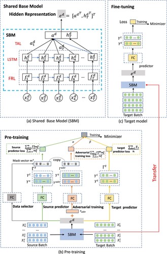
In this paper, we propose a novel Selective Transfer Learning framework with Adversarial Training (STLAT) for stock movement prediction. Overview of the proposed STLAT is provided in Figure 1. The main working process is shown as follows: (i) the source batch from source domain is fed into the Shared Base Model (SBM) to produce the hidden representation $e^d$. SBM is an attention-based LSTM network which is illustrated in Figure 1(a). (ii) Three different tasks, which are shown in the left of Figure 1(b), acting on $e^d$ and generating the prediction results. More specifically, the data selector is employed to select data from source batch aiming at introducing more beneficial samples to improve the prediction results of target stock. The source predictor is introduced to measure the performance of source batch. The adversarial training, adding the slight perturbation to $e^d$, is applied to improve the generalisation of the model SBM. (iii) SBM is then updated with the selected training samples from source batch. The target batch from target domain is fed into the previously trained SBM to get the target predictor loss shown in the right of Figure 1(b), which is used to measure the effectiveness of the current data selector. (iv) SBM is next jointly trained by the total loss with the same source batch and the target batch, which is the combination of the source predictor loss, adversarial training loss and target predictor loss. (v) Finally, the pre-trained SBM is transferred to the target model in the fine-tuning process, which is shown in Figure 1(c). All the end-to-end parameters of the target model is trained with the target batch from the target stock. Moreover, the test data of target stock is evaluated on the target model.

Figure 1. (Better viewed in colour) The overview of our proposed architecture STLAT. The target batch in (b) represents the validated samples from target stock and the target batch in (c) represents the training samples from target stock.

The main contributions of this paper are threefold.

• We propose a novel selective transfer learning framework with adversarial training to address the problem of weak generalisation of the model in the field of stock movement prediction.

• We introduce two steps within the framework: pre-training and fine-tuning. A data selector is utilised to effectively choose source domain data for transfer learning. Furthermore, adversarial training is employed to improve the generalisation of SBM.

• We conduct extensive experiments on two public benchmarks and a newly constructed dataset. Experiments demonstrate that our proposed framework outperforms a number of competitive baselines and achieves state-of-the-art performance.

2. Related work

2.1. Stock movement prediction

As a subset of time series predictions, stock movement prediction has attracted both investors and researchers. Several methods used for time series prediction can be roughly divided into the following two categories: traditional linear predicting methods and nonlinear predicting methods. Linear predicting methods include auto regression (AR), moving average (MA), auto regressive integrated moving average (ARIMA) (Saboia, 1977) and so on. However, the financial time series data is non-linear, which makes the traditional linear predicting methods be struggling in accurate prediction. Recently, machine learning and deep learning techniques (D'Angelo et al., 2021; Kamilaris & Prenafeta-Boldú, 2018; Ying, Qian Nan et al., 2021) have been widely applied in many fields. Especially, Jiang (2021), Nti et al. (2020) and Wu, X. et al. (2021) have drawn the growing attention in financial time series prediction tasks due to their capability in nonlinear mapping and generalisation (Chen & Tan, 2021; Feng, Chen et al., 2019; Feng, He et al., 2019; Khuwaja et al., 2021; Tran et al., 2019). For instance, Nti et al. (2021) present a novel multi-source information-fusion predictive framework for enhancing the accuracy in stock market prediction. Lin et al. (2021) present a model to enhance the existing stock prediction with the ability to model multiple stock trading patterns. Meanwhile, several studies exploit extra market information, like event information, social media information into the prediction (Camacho et al., 2021; Ding et al., 2015; Jin et al., 2020; Wang et al., 2021; Xu & Cohen, 2018). For instance, Sawhney et al. (2021) used the valuable rich signals between related stocks' movements to construct the hyperbolic graph for algorithmic trading. Wu, S. et al. (2021) present a framework that framework incorporating multiple data sources and investors' sentiment to predict stock price. Our work falls into the nonlinear predicting methods without extra information.

In the field of stock movement prediction, fundamental analysis and technical analysis are the two basic methods. Fundamental analysis attempts to measure the intrinsic value of a stock by examining related economic, financial and other qualitative and quantitative factors (Bollen et al., 2011; Ding et al., 2015; Xu & Cohen, 2018). Technical analysis tends to take the historical market data to predict its future movement with advanced models in recent years (Feng, Chen et al., 2019; Li et al., 2019; Qin et al., 2017). Our work falls into the technical analysis.

2.2. Adversarial training

Adversarial training (Goodfellow et al., 2015) can reveal the defects of models and improve the robustness. The main process of adversarial training is to inject adversarial examples designed by an adversary to increase the robustness of the model. Most adversarial examples are generated by adding small perturbation to clean samples. Previous studies primarily applied adversarial training to image classification tasks (Goodfellow et al., 2015; Miyato et al., 2016; Xie et al., 2017). Recently, the adversarial training has also been used to text classification (i.e. applying perturbations to the word embedding) (Miyato et al., 2017), recommendation (i.e. adding adversarial perturbations on model parameters to maximise the Bayesian personalised ranking objective function) (He et al., 2018), graph node classification (i.e. modifying the combinatorial structure of data) (Dai et al., 2018), multi-agent reinforcement learning (Li et al., 2021). Meanwhile, Feng, Chen et al. (2019) explore the potential of adversarial training in stock price prediction, small perturbations are added to the hidden representation to improve the generalisation of the model. The experiments confirm the effectiveness of adversarial training for the stock movement prediction task. Therefore, to address the highly stochastic property of stock price, we apply the adversarial training to the prediction model. Nevertheless, we apply the Kullback–Leibler divergence cost function in adversarial training, which can improve the predictions results compared to Feng, Chen et al. (2019).

2.3. Transfer learning

Transfer Learning has been widely investigated in the past years (Cao et al., 2021; Weiss et al., 2016; Ying, Qiqi et al., 2021). Different from traditional machine learning methods, in which training data and test data must follow the same distribution, transfer learning can utilise knowledge from other domains for new relevant domains (Ye & Dai, 2018). Existing research in domain adaptation has been successfully applied to fields including text sentiment classification (Wang & Mahadevan, 2011), image classification (Oquab et al., 2014; You et al., 2015), human activity classification (Harel & Mannor, 2011) and so on. Recently, BERT (Devlin et al., 2019) has also demonstrated the importance of transfer learning from large pre-trained models, where an effective method is to fine-tune models. In the field of time series analysis, since each stock has small data in terms of daily data, transfer learning is the key to help deep learning techniques in a large number of different stock data settings. Recently, He et al. (2019) proposes a similarity-based approach for selecting source datasets to train the deep learning models with transfer learning. It shows that transfer learning can be effectively used for financial time series forecasting. The study (Nguyen & Yoon, 2019) proposes a deep transfer-based framework to predict the stock price movement. It demonstrates the effectiveness of transfer learning and using stock relationship information in helping to improve model performance. However, both these two approaches lack of an effective data selection method. In particular, not all the relational stock data is suited for the movement prediction of target stock.

In this paper, we propose an effective transfer learning framework incorporating an automatic data selection. The process of data selection is not pre-defined like previous studies. To the best of our knowledge, this paper is the first work to explore the potential of data selection which is jointly trained with transfer learning in the field of stock movement prediction.

2.4. Problem statement

Stock movement prediction task is to learn a prediction function $Y=f(X,\theta )$, where θ is the parameter and $Y\in (-1,1)$ denotes the stock movement. Specifically, given the sequential features $X=[x_1,x_2,\dots ,x_T]$, where $x_i\in {\mathbb{R}}^D$ and D is the variable dimension, We are interested in predicting the movement at a certain future moment, i.e. predicting the movement of $x_{T+h}$, where h is the desirable horizon ahead of the current time stamp. In our experiments, h is set to 1, which means predicting the stock movement at next day. Moreover, the training samples are fed into the model through batch level. We denote the specific training sample i in a batch by $X_i$ and the prediction result by $Y_i$.

3. Our model

3.1. Shared base model (SBM)

As illustrated in Figure 1(b and c), model SBM in STLAT is an attention-based LSTM network. It is pre-trained with the source batch from source domain and fine-tuned with the target batch from target domain. Note that the proposed STLAT can integrate different shared base models. The attention-based LSTM network contains feature representation layer, LSTM layer and temporal attention layer.

3.1.1. Feature representation layer (FRL)

Feature representation layer is a feature learning technique which maps sequential features to latent representation. Formally, we denote the input sequential features of a training sample i in a batch by $X_i^d=[x_1^d,x_2^d,\dots ,x_T^d]$, where $d\in \{s,t\}$ represents the source domain or target domain and T is the latest time-steps. We employ a fully connected layer to map $x_t^d$ into a latent representation denoted by $f_t^d$, which is computed as $f_t^d=\tanh (W_f{x}_t^d+b_f)$, where $W_f$ and $b_f$ are parameters to be learned. The main reason is that previous work (Wu et al., 2018) shows that a deeper input gate would benefit the modelling of temporal structures of LSTM in next section.

3.1.2. LSTM layer

LSTM (Hochreiter & Schmidhuber, 1997) is one of the most representative variations of recurrent neural network (RNN) architecture. It has been widely used in time series modelling since it can overcome the problem of vanishing gradients and better capture long-term dependencies of time series (Li et al., 2019; Qin et al., 2017). For stock movement prediction, at each time-step, LSTM is applied here to learn a mapping from latent representation $f_t^d$ and previous hidden state $h_{t-1}^d$ to a hidden representation denoted by $h_t^d$. We formulate it as $h_t^d=\mathsf{L}\mathsf{S}\mathsf{T}\mathsf{M}(f_t^d,h_{t-1}^d)$. Overall, $[f_1^d,f_2^d,\dots ,f_T^d]$ is mapped to the hidden representation $[h_1^d,h_2^d,\dots ,h_T^d]$.

3.1.3. Temporal attention layer (TAL)

Although the LSTM layer can learn long-term dependencies, it is struggling to determine which time instances are more important to the prediction. Recent work (Cinar et al., 2017) shows that the attention-based model can make use of the (relative) positions in the sequential inputs and perform better than the model without attention mechanism. In order to learn the importance of each time instance for stock representation, we use the temporal attention augmented LSTM that maps the hidden representation $h_t^d$ to the aggregated representation $a^d$. This process can be expressed as follows: (1) $\begin{array}{rl}{\tilde{a}}_t^d& =u_a^T\tanh (W_a{h}_t^s+b_a),\end{array}$(1) (2) $\begin{array}{rl}{a}_t^d& =\frac{\exp ({\tilde{a}}_t^d)}{\sum _{t=1}^T\exp ({\tilde{a}}_t^d)},\end{array}$(2) (3) $\begin{array}{rl}{a}^d& =\sum _{t=1}^T{a}_t^d{h}_t^d,\end{array}$(3) where $W_a$, $u_a$ and $b_a$ are parameters to be learned. Motivated by Fama and French (2012), to generate quantile predictions from hidden states, we concatenate $a^d$ with the last hidden representation $h_T^s$ into the final latent representation denoted by $e^d=[{a^d}^T,{h_T^s}^T{]}^T$.

3.2. Pre-training

3.2.1. Predictor

We use a fully connected layer as the predictive function to estimate the classification task of stock movement prediction. Note that, the training samples are fed into the model through batch level, where the batchsize is denoted by n. If the training samples $[X_1,X_2,\dots ,X_n]$ are from source domain, we denote the prediction results by $Y^s=[Y_1^s,Y_2^s,\dots Y_n^s]$; if the training samples are from target domain, we denote the prediction results by $Y^t=[Y_1^t,Y_2^t,\dots Y_n^t]$. $Y^l=[Y_1^l,Y_2^l,\dots Y_n^l]$ is the label of stock price movement. Therefore, the source predictor loss is ${\mathrm{\Gamma }}^s=[{\mathrm{\Gamma }}_1^s,{\mathrm{\Gamma }}_2^s,\dots ,{\mathrm{\Gamma }}_n^s]$, where ${\mathrm{\Gamma }}_i^s\in {\mathrm{\Gamma }}^s$ is the cross-entropy loss, i.e. ${\mathrm{\Gamma }}_i^s=-Y_i^l\log (Y_i^s)-(1-Y_i^l)\log (1-Y_i^s)$. Moreover, the target predictor loss is ${\mathrm{\Gamma }}^t=[{\mathrm{\Gamma }}_1^t,{\mathrm{\Gamma }}_2^t,\dots ,{\mathrm{\Gamma }}_n^t]$.

3.2.2. Adversarial training

Adversarial training (Goodfellow et al., 2015) is a novel regularisation method for classifiers to improve robustness by adding a subtle perturbation to the inputs, it meets with the success in image classification (Kurakin et al., 2017) and text classification (Miyato et al., 2017). They usually add the perturbations to the input image or text embedding directly to learn a robust model. However, it may break the sequential relation of the stock price with different LSTM units thereby causing the uncontrollable input. Considering that the model can capture the noises by enhancing the predictions on different aggregated representation, we add the perturbations $r_{\mathsf{a}\mathsf{d}\mathsf{v}}^d$ into the final aggregated representation $e^d$ of the SBM. Thus the final adversarial example is $a_{\mathsf{a}\mathsf{d}\mathsf{v}}^d=e^d+r_{\mathsf{a}\mathsf{d}\mathsf{v}}^d$. The adversarial training follows the cost function Kullback–Leibler divergence motivated by Miyato et al. (2017), (4) ${\mathrm{\Gamma }}^{\mathsf{a}\mathsf{d}\mathsf{v}}=\text{KL}(Y^{\mathsf{a}\mathsf{d}\mathsf{v}},Y^s)=\text{KL}[p(\cdot |e^d;\hat{\theta })||p(\cdot |e^d+r_{\mathsf{a}\mathsf{d}\mathsf{v}}^d;\hat{\theta })],$(4) where ${\mathrm{\Gamma }}^{\mathsf{a}\mathsf{d}\mathsf{v}}$ is a vector containing the loss of each training sample, $r_{\mathsf{a}\mathsf{d}\mathsf{v}}^d=\text{arg}\underset{r,\Vert r\Vert \le ϵ}{max}\text{KL}[p(\cdot |e^d;\hat{\theta })||p(\cdot |e^d+r;\widehat{\theta )}]$ and $\text{KL}[P||Q]=\sum p(x)\log \frac{p(x)}{q(x)}$ denotes the KL divergence between distributions P and Q, ϵ is a hyper-parameter to control the scale of perturbation. To approximate the perturbations value, we employ the fast gradient approximation method (Goodfellow et al., 2015), with the $L_2$ norm constraint in the KL loss. The perturbation and parameters can be updated using back propagation in our proposed SBM as follows: (5) $r_{\mathsf{a}\mathsf{d}\mathsf{v}}^d=\epsilon g/\Vert g{\Vert }_2$(5) where g can be obtained by (6) $g={▽}_{e^d}\text{KL}[p(\cdot |e^d;\hat{\theta })||p(\cdot |e^d+r_{\mathsf{a}\mathsf{d}\mathsf{v}}^d;\hat{\theta })].$(6)

3.2.3. Data selector

After performing prediction task and adversarial task on the source domain, we argue that no all source training samples are beneficial for improving the prediction performance of target stock. Therefore, we propose a data selector to select the beneficial training samples. More specifically, data selector is a fully connected layer on the top of the SBM. Unlike the predictor task, the output of data selector task is a mask vector $m^s=[m_1^s,m_2^s,\dots ,m_n^s]$ containing 1(0)s representing whether to select a training sample from source batch. Figure 1(b) shows how the data selection module affects the source predictor and adversarial training. Formally, if a training sample $X_i^s$ is selected to update model SBM, the output of $m_i^s$ is 1. Here, we directly apply m to the loss ${\mathrm{\Gamma }}^s$ and ${\mathrm{\Gamma }}^{\mathsf{a}\mathsf{d}\mathsf{v}}$ to formulate them and simply calculate them by dot product as ${\mathrm{\Gamma }}^s\cdot m$, ${\mathrm{\Gamma }}^{\mathsf{a}\mathsf{d}\mathsf{v}}\cdot m$, respectively. More specifically, if a training sample is selected, the corresponding loss will be added in the total source loss. Otherwise, the corresponding loss will be removed. At last, we denote the average of the total source loss by ${\mathrm{\Gamma }}^{se}$ and it is calculated as follows: (7) ${\mathrm{\Gamma }}^{se}=\frac{\sum _{i=1}^n({\mathrm{\Gamma }}_i^s+\alpha {\mathrm{\Gamma }}_i^{\mathsf{a}\mathsf{d}\mathsf{v}})m_i^s}{\sum _{i=1}^n{m}_i^s},$(7) where α is the hyper-parameter and ${\mathrm{\Gamma }}^{se}$ is the average of the total source loss because the number of source training samples are selected differently in the total source loss during each training step. The performance of the data selector is evaluated by the performance of the target batch from target domain. If the performance of the target batch is better after updating the model with the selected source training samples, it can show the effectiveness of the data selector. Here, we add the target predictor loss to guide the learning of data selector. The training details is described as follows.

3.2.4. Pre-training process

At each training step, the pre-training of the proposed model works as follows: for a target stock, (i) the source batch from source stocks is fed into the source predictor task, adversarial training task and data selector task, thereby getting the prediction results $Y^s$, $Y^{\mathsf{a}\mathsf{d}\mathsf{v}}$ and $m^s$. (ii) We then update the SBM with loss ${\mathrm{\Gamma }}^{se}$ in Equation (7(7) ${\mathrm{\Gamma }}^{se}=\frac{\sum _{i=1}^n({\mathrm{\Gamma }}_i^s+\alpha {\mathrm{\Gamma }}_i^{\mathsf{a}\mathsf{d}\mathsf{v}})m_i^s}{\sum _{i=1}^n{m}_i^s},$(7) ). (iii) The same source batch and the target batch from target stock are fed into the source predictor task, adversarial training task, data selector task and target predictor, thereby getting another prediction results $Y^s$, $Y^{\mathsf{a}\mathsf{d}\mathsf{v}}$, $m^s$ and $Y^t$, respectively. The reason of steps (ii) and ( iii) is that the target predictor loss should be calculated after SBM trained with selected training samples. (iv) At last, we compute the total objective function Γ in and update all the parameters of the pre-training model. Γ is calculated as follows: (8) $\begin{array}{rl}\mathrm{\Gamma }& ={\mathrm{\Gamma }}^{se}+\beta \frac{\sum _{i=1}^n{\mathrm{\Gamma }}_i^t}{n}+\frac{\gamma }{2}{L}_2\\ & =\frac{\sum _{i=1}^n({\mathrm{\Gamma }}_i^s+\alpha {\mathrm{\Gamma }}_i^{\mathsf{a}\mathsf{d}\mathsf{v}})m_i^s}{\sum _{i=1}^n{m}_i^s}+\beta \frac{\sum _{i=1}^n{\mathrm{\Gamma }}_i^t}{n}+\frac{\gamma }{2}\Vert \theta {\Vert }_2,\end{array}$(8) where the term α, β and γ are the hyper parameters to balance the different losses. More specifically, ${\mathrm{\Gamma }}^{se}$ is in Equation (7(7) ${\mathrm{\Gamma }}^{se}=\frac{\sum _{i=1}^n({\mathrm{\Gamma }}_i^s+\alpha {\mathrm{\Gamma }}_i^{\mathsf{a}\mathsf{d}\mathsf{v}})m_i^s}{\sum _{i=1}^n{m}_i^s},$(7) ), ${\mathrm{\Gamma }}^{\mathsf{a}\mathsf{d}\mathsf{v}}$ is in Equation (4(4) ${\mathrm{\Gamma }}^{\mathsf{a}\mathsf{d}\mathsf{v}}=\text{KL}(Y^{\mathsf{a}\mathsf{d}\mathsf{v}},Y^s)=\text{KL}[p(\cdot |e^d;\hat{\theta })||p(\cdot |e^d+r_{\mathsf{a}\mathsf{d}\mathsf{v}}^d;\hat{\theta })],$(4) ). We also introduce a $L_2$ norm constraint in the objective function.

3.3. Fine-tuning

Fine-tuning is straightforward to use the parameters in the SBM, which are initialised after the process of the pre-training, as depicted in the red arrow as shown in Figure 1. Meanwhile, we build a fully connected layer in the above of the SBM as the target model to predict the labels. The training process is to minimise the cross-entropy loss between $Y^t$ and $Y^l$ of target stock training data. Thus we fine-tune all the end-to-end parameters of the target model. Compared to pre-training, fine-tuning is relatively inexpensive, since the parameters are slightly updated to fit the target stock training data. Lastly, we use the target model to evaluate the testing data from target stock.

3.3.1. Training process

Our framework under the transfer learning schema is trained as the following procedure. We adopt the leave-one-out strategy to construct the source domain data for pre-training and the target domain data for fine-tuning. First, for an individual target stock in the dataset, all the remaining stocks except the target stock are utilised as source stocks. Second, in the pre-training stage, for each training batch in source domain stocks, we randomly select target training batch because the number of source training batches is much larger than the number of target training batches. Third, in the fine-tuning stage, we construct the target model based on the pre-trained SBM and fine-tune all the end-to-end parameters of the target model. The detailed training process is described in Algorithm 1.

4. Experiments

4.1. Data description

In this paper, we evaluate the performance of our proposed STLAT model on three benchmarks on stock movement prediction. Two of the three benchmarks are provided from ACL18 (Xu & Cohen, 2018) and KDD17 (Zhang et al., 2017). For the ACL18 dataset, 88 high-trade-volume stocks in U.S. market are selected. We split the dataset into training set (2014-01-01 to 2015-08-01), validation set (2015-08-01 to 2015-10-01) and testing set (2015-10-01 to 2016-01-01). For the KDD17 dataset, 50 top-capitalisation stocks in U.S. market are selected. We split the dataset into training (2007-01-01 to 2015-01-01), validation (2015-01-01 to 2016-01-01), and testing (2016-01-01 to 2017-01-01).

In addition, we introduce a new stock dataset collected from Chinese stock market, denoted by CN50. We follow the same data collection approaches as the KDD17 dataset, while using the Chinese market instead of the U.S. market. Finally, 50 stocks in 10 industries are collected and each stock has top capitalisation in the corresponding industry. We also split the dataset into training set (2010-01-01 to 2018-01-01), validation set (2018-01-01 to 2019-01-01) and testing set (2019-01-01 to 2020-01-01).

In the preprocessing stage, we create features for modelling the market state for each trading day. Specifically, we utilise the 11 features described in Adv-LSTM (Feng, Chen et al., 2019) and involve 10 auxiliary features. These technical features indicate the moving average or the rate of change of stock market. The details of all these features are elaborated in Table 1.

Table 1. Technical features used in the model and their calculation. ma: moving average. roc: rate of change.

Features	Calculation
c_open, c_high, c_low	c_open=${\mathsf{o}\mathsf{p}\mathsf{e}\mathsf{n}}_t/{\mathsf{c}\mathsf{l}\mathsf{o}\mathsf{s}\mathsf{e}}_t-1$
5-ma, 10-ma, 15-ma,	n-ma=$\frac{{\sum }_{i=0}^{n-1}\mathsf{a}\mathsf{d}\mathsf{j}\mathrm{\_}{\mathsf{c}\mathsf{l}\mathsf{o}\mathsf{s}\mathsf{e}}_{t-i}}{\mathsf{a}\mathsf{d}\mathsf{j}\mathrm{\_}{\mathsf{c}\mathsf{l}\mathsf{o}\mathsf{s}\mathsf{e}}_t}-1$
20-ma, 25-ma, 30-ma
1-roc, 5-roc, 10-roc,	n-roc=$\frac{{\mathsf{c}\mathsf{l}\mathsf{o}\mathsf{s}\mathsf{e}}_t}{{\mathsf{c}\mathsf{l}\mathsf{o}\mathsf{s}\mathsf{e}}_{t-n}}-1$
15-roc, 20-roc, 25-roc
1-roc', 5-roc', 10-roc',	n-roc'=$\frac{\mathsf{a}\mathsf{d}\mathsf{j}\mathrm{\_}{\mathsf{c}\mathsf{l}\mathsf{o}\mathsf{s}\mathsf{e}}_t}{\mathsf{a}\mathsf{d}\mathsf{j}\mathrm{\_}{\mathsf{c}\mathsf{l}\mathsf{o}\mathsf{s}\mathsf{e}}_{t-n}}-1$
15-roc', 20-roc', 25-roc'

Finally, at the trading day t, the associated example has 21 temporal features that are labelled with negative or positive according to the movement percentage p $\le -0.5\mathrm{\%}$ or $\ge 0.55\mathrm{\%}$, respectively, where $p=\mathsf{a}\mathsf{d}\mathsf{j}\mathrm{\_}{\mathsf{c}\mathsf{l}\mathsf{o}\mathsf{s}\mathsf{e}}_{t+1}/\mathsf{a}\mathsf{d}\mathsf{j}\mathrm{\_}{\mathsf{c}\mathsf{l}\mathsf{o}\mathsf{s}\mathsf{e}}_t-1$. This leaves us the total samples of three datasets divided as 48.62% and 51.38% in the two classes. Note that $\mathsf{a}\mathsf{d}\mathsf{j}\mathrm{\_}\mathsf{c}\mathsf{l}\mathsf{o}\mathsf{s}\mathsf{e}$ represents the adjusted closing price that modifies a stock's closing price to exactly reflect that stock's value after accounting for some corporate actions, such as stock splits and stock dividends.

4.2. Baselines and metrics

We compare our model with the following baselines:

• RAND: a simplest predictor making random guess (up or down) and each direction has an equal probability.

• ARIMA (Brown, 2004): Autoregressive Integrated Moving Average models historical prices as a nonstationary time series.

• RF (Kumar & Thenmozhi, 2006): A random forest classifier, which makes decision according to features, is a popular ensemble model.

• LSTM (Hochreiter & Schmidhuber, 1997): Long Short Term Memory network, a special RNN model.

• DA-RNN (Qin et al., 2017): The temporal attention mechanism is applied to the LSTM-based model, we convert the regression predictor of the model to the classification predictor to suit our problem.

• SFM (Zhang et al., 2017): a novel State Frequency Memory (SFM) recurrent network to capture the multi-frequency trading patterns from past market data to make long and short term predictions over time.

• S-TF (He et al., 2019): It introduces a similarity-based approach for selecting source stocks for training the target stock. The base model of S-TF is LSTM.

• Adv-ALSTM (Feng, Chen et al., 2019): It is an attention-based LSTM network which uses adversarial training and performs better than ALSTM.

• MAN-SF (Sawhney et al., 2020): It introduces an architecture that combines a potent blend of chaotic temporal signals from financial data, social media, and inter-stock relationships via a graph neural network in a hierarchical temporal fashion, which is the state-of-the-art model.

• STLAT (w/o AT): STLAT without adversarial training.

• STLAT (w/o TL): STLAT without transfer learning.

• STLAT (w/o S): STLAT without source data selector.

Following previous work on stock prediction (Ding et al., 2015), two standard metrics of accuracy (Acc) and Matthews Correlation Coefficient (MCC) are adopted for evaluating the prediction performance. Higher Acc and MCC indicate better performance.

4.3. Implementation details

4.3.1. Model configuration

Several hyper-parameters are involved in our framework and each has its impact. For searching the optimal hyper-parameters, we tweak them according to the performance on the validation set. Specifically, we tune the LSTM hidden units, the time-step lag size via grid-search within the list of $lh\in \{4,8,20,50,100,200\}$ and $\iota \in \{5,8,10,15,20,25\}$. Following Feng, Chen et al. (2019), we tune the perturbation scale via grid-search of $ϵ\in \{0.001,0.005,0.01,0.05,0.1,0.5\}$. And we also tune the training loss factors α, β and γ within the list of $\{0.05,0.1,0.3,0.5,1\}$, $\{0.05,0.1,0.3,0.5,1\}$ and $\{0.05,0.1,0.3,0.5,1\}$, respectively. Finally, the optimised parameters used to obtain the final result of STLAT in Table 2 are as follows: for ACL18, lh = 20, $\iota =15$, $ϵ=0.005$. For KDD17, lh = 20, $\iota =10$, $ϵ=0.01$. For CN50, lh = 20, $\iota =8$, $ϵ=0.01$. $\alpha =0.3$, $\beta =0.5$ and $\gamma =1$ are suited for three datasets.

Table 2. Experimental results (Acc and MCC) comparison of our model and baselines on three stock benchmarks.

	ACL18		KDD17		CN50
Model	ACC(%)	MCC	ACC(%)	MCC	ACC(%)	MCC
RAND	49.72	−0.0056	50.09	0.0018	49.88	−0.0023
ARIMA (Brown, 2004)	51.03	−0.0021	50.28	−0.0053	50.83	0.0437
RF (Kumar & Thenmozhi, 2006)	52.13	0.0112	51.18	0.0208	51.73	0.0410
LSTM (Hochreiter & Schmidhuber, 1997)	53.19	0.0136	51.62	0.0183	51.16	0.0393
DA-RNN (Qin et al., 2017)	54.90	0.1043	51.94	0.0261	51.80	0.0433
SFM (Zhang et al., 2017)	56.12	0.1242	52.10	0.0277	52.11	0.0506
S-TF (He et al., 2019)	56.68	0.1323	52.71	0.0289	52.14	0.0512
Adv-ALSTM (Feng, Chen et al., 2019)	57.20	0.1483	53.05	0.0523	52.16	0.0515
MAN-SF (Sawhney et al., 2020)	60.80	0.1950	54.15	0.0621	53.44	0.0860
STLAT-AT	60.61	0.2240	55.73	0.1110	56.01	0.1178
STLAT-TL	58.78	0.1698	54.57	0.0864	54.86	0.0914
STLAT-S	61.44	0.2394	56.08	0.1233	56.78	0.1363
STLAT	64.56	0.2967	58.27	0.1585	58.33	0.1636

4.3.2. Training protocol

Different from the baselines, our framework is under the transfer learning schema. We adopt the leave-one-out strategy to construct the source domain data for pre-training and the target domain data for fine-tuning. First, for an individual stock S in the dataset, all the remaining stocks except S are utilised in the pre-training stage. Second, we fine-tune S based on the pre-trained model and obtain the performance on testing set with the best validation performance on the model. The final performance of dataset is an average result of all contained stocks.

We train our model's parameters using gradient-based optimiser Adam, with an initial learning rate 0.01 and a batch size of 128. We set 200 epochs for the pre-training stage and fine-tune the model with 200 additional epochs. To avoid overfitting, early stopping strategy is adopted during the training process.

4.4. Results

We show the performance of the baselines and our proposed model in Table 2. From the results, we observe that our model achieves both best Acc and MCC on three datasets. The RAND predictor achieves accuracy around 50/50 percent as we expect. LSTM slightly outperforms RF on ACL18 and KDD17. DA-RNN outperforms LSTM, indicating the validity of the attention mechanism. S-TF outperforms LSTM, which shows the effectiveness of data selection though it uses a simple similarity based method to select training samples. SFM introduces the frequency-aware sequential embeddings, which help it outperforms DA-RNN and LSTM. Adv-ALSTM shows better performance, this is because it introduces the adversarial training to the prediction model.

Significantly, our model outperforms previous state-of-the-art model MAN-SF by a large margin. The proposed STLAT achieves the best accuracy 64.56 (6.18%↑) on ACL18, 58.27 (7.60%↑) on KDD17 and 58.33 (9.15%↑) on CN50 despite social media, and inter-stock relationships are introduced to MAN-SF, which is the best baseline. The main reason is that we introduce the transfer learning mechanism and make an effective data selector to enhance the prediction. Meanwhile, our model achieves analogical improvement on the performance of MCC. The results demonstrate consistently better performance, which indicates the effectiveness and robustness of our STLAT.

Moreover, to make an elaborate analysis of all the primary components within our proposed framework, we construct some variations of STLAT. The results are shown in Table 2. Comparing with the full model STLAT, we can observe that eliminating any of the proposed modules would hurt the performance significantly. More specifically, removing the transfer learning (pre-training stage) leads to the largest accuracy decrease on all datasets. This observation shows the advantage of transfer learning in stock movement prediction. Meanwhile, the data selector contributes to the best performance because of its ability to determine which source domain training samples are beneficial for transferring. Furthermore, adversarial training is also a convincing strategy to enhance the generalisation, which constrains the prediction to be consistent among slight perturbation. Note that model STLAT-TL slightly outperforms the Adv-ALSTM. The main reason lies in the adoption of KL divergence loss instead of the hinge loss, which demonstrates the effectiveness of the designed KL divergence loss. The results reveal the effectiveness of each proposed component and the elaborate full framework STLAT.

We also calculate other metrics for further comparison with the best two baselines on the ACL18 dataset. Metrics include specificity, precision, sensitivity and f1 score. The results are shown in Table 3. From the results, we observe that our model achieves the best results on all four metrics among the two best baselines, which demonstrates the effectiveness of our model. Meanwhile, the best baseline MAN-SF does not outperform the Adv-ALSTM model on all metrics. Although due to the pre-training and fine-tuning process, the proposed STLAT architecture looks a bit complicated. For a stock, the training and prediction time of our model is close to other baselines.

Table 3. Performance with different metrics on ACL18 dataset.

Model	Specificity (%)	Precision (%)	Sensitivity (%)	F1-score (%)
Adv-ALSTM (Feng, Chen et al., 2019)	59.41	56.22	60.10	58.09
MAN-SF (Sawhney et al., 2020)	58.11	61.44	58.16	59.75
STLAT	63.14	65.15	63.19	64.15

4.5. Impact of parameters

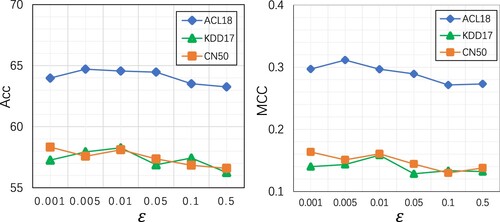
We further discuss the effect of hyper-parameters on our model STLAT. We first investigate the impact of perturbation control factor. We vary its value as $ϵ\in \{0.001,0.005,0.01,0.05,0.1,0.5,1\}$ in different scales. As shown in Figure 2, the optimal value of ϵ is associated with the best performance around the mid-section of value range. This result indicates that too small or too large perturbation of the adversarial training cannot benefit the robustness of model. Moreover, the performance of three benchmarks has different peak values (in terms of $\mathsf{A}\mathsf{c}\mathsf{c}$ and $\mathsf{M}\mathsf{C}\mathsf{C}$), implying that stocks in diverse markets have different noise tolerance values.

Figure 2. Impact of the perturbation scale.

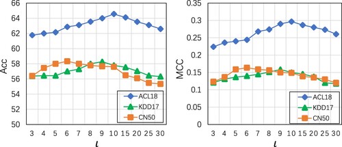
To demonstrate the impact of the time-step lag size, we vary its value as $\iota \in \{3,4,5,6,7,8,9,10,15,20,25,30\}$. As shown in Figure 3, the optimal value of ι is associated with the best performance around $8\sim 10$ on ACL18 and KDD17. This indicates that too small or too large time-step lag size cannot benefit the prediction of model. The main reason is that data from a long time ago has little impact on current forecasting and small size time-step may lose some effective information. Moreover, the performance ($\mathsf{A}\mathsf{c}\mathsf{c}$ and $\mathsf{M}\mathsf{C}\mathsf{C}$) of ACL18 and KDD17 datasets almost has the same peak value, but the performance of CN50 has a different peak value compared to them, implying that stocks in different markets (U.S and China) have different characteristics.

Figure 3. Impact of the time-step lag size.

4.6. Impact of data selector

To make an elaborate analysis of the impact of data selector module in our proposed framework, we collect a full stock list in S&P 500, which includes 500 large companies in the United States and contains 11 sectors, 24 industry groups, 67 industries and 156 sub-industries in 2019. Furthermore, S&P 500 is one of the best representations of the U.S. stock market. We have compared four strategies based on our STLAT model for testing the effectiveness of data selector in financial time series forecasting. These strategies are numbered from $S_1$ to $S_4$. All these strategies utilise the leave-one-out strategy to construct the source domain data for pre-training and the target domain data for fine-tuning. The selection of source domain data is described as follows:

• $S_1$: full stocks without selection

• $S_2$: selection according to market capitalisation.

• $S_3$: selection according to sector.

• $S_4$: selection according to historical similarity.

The first strategy $S_1$ is to train the STLAT with all stocks in S&P 500. The second strategy $S_2$ divides all stocks equally into 10 groups by market capitalisation. For instance, for each target stock in the first group, the number of source domain stocks is 49. Similarly, the third strategy $S_3$ divides all stocks into 24 groups according to the aforementioned partition criterion of S&P 500. The last strategy $S_4$ selects the top 10% most similar (computed by Cosine similarity) stocks for each target stock.

Table 4 shows the comparison of strategies with data selector or without on S&P500. The term $S_k$+DS represents the kth strategy that utilises data selector. The performance in the table is an average result of all contained stocks. From Table 4, we have the following observations: (i) All strategies with data selector achieve the better results compared to those without data selector. This justifies the effectiveness of data selector, which might be due to the selection of the most relevant time series to enhance the prediction. (ii) Improper selection of source domain stocks may lead to a decrease in accuracy when compared $S_2$ and $S_1$. (iii) In all cases without data selector, we find that $S_4$ achieves the best performance. The main reason is that source domain stocks have a better correlation with the target stock than the other strategies.

Table 4. Performance in Acc / MCC is reported with four strategies.

Model	ACC (%)	MCC
$S_1$ / $S_1$+DS	58.45 / 60.16	0.1672 / 0.2284
$S_2$ / $S_2$+DS	57.61 / 59.38	0.1438 / 0.2026
$S_3$ / $S_3$+DS	62.78 / 63.44	0.2631 / 0.2845
$S_4$ / $S_4$+DS	63.14 / 64.87	0.2710 / 0.3041

4.7. Discussion

In this section, we will conduct an in-depth analysis of our proposed method. It contains three aspects, namely main findings, limitations and industrial significance.

For the main findings, we found that transfer learning is helpful for stock trend prediction, especially when introducing the most relevant training samples through the data selector module. It can be explained that investors may use the same strategy for different stocks at different times, causing the others stock training samples can be helpful for the specific stock. In addition, adversarial training can also improve the generalisation ability of neural network prediction models, which is helpful for stock movement prediction.

For the limitations, introducing relevant training samples from other stocks can indeed improve the accuracy of stock movement prediction. In this paper, we use an efficient data selector to improve the prediction. However, it lacks interpretability and cannot figure out which trading patterns can be helpful. The interpretability is important to the investment field, and this is also our focus in the future.

For the industrial sense, investors can make or lose to a large extent depending on whether they can make correct predictions about stock movements. Usually, they treat each stock independently and miss a lot of useful information that other stocks can provide. Our STLAT model provides a new perspective to investors and can help them make good investment decisions.

5. Conclusion and future work

In this paper, we propose a novel framework (STLAT) with selective transfer learning and adversarial training for stock movement prediction. STLAT applies transfer learning to effectively utilise source domain data based on the data selector to filter out useless source data and prevent negative transfer. Adversarial training is also exploited to improve the generalisation against the stochasticity of stock. Experiments demonstrate that the proposed approach outperforms competitors and achieves state-of-the-art results. Ablation and parameter analyses also reveal the effectiveness of our framework.

In the future, we intend to explore the following researches: (i) there exists the right prediction that may make a small profit while the wrong prediction may make a large loss. Thus a forecasting scheme that has achieved a large number of successful predictions can even cause a loss. In the future, we will exploit the solutions towards optimising the target of investment, i.e. selecting the best stock with the highest expected revenue. (ii) This paper only considers historical stock prices to predict the future movement directions while other factors such as market sentiment and political events can also affect the stock movement. In the future, we will leverage external data derived from news, financial and political events for better prediction.

Disclosure statement

No potential conflict of interest was reported by the authors.

Additional information

Funding

The research is supported by the Key-Area Research and Development Program of Guangdong Province (No. 2020B010165003), and the National Natural Science Foundation of China (No. U1811462), Macao Science and Technology Development Fund under Macao Funding Scheme for Key R & D Projects (0025/2019/AKP), and Hong Kong Institute of Business Studies (HKIBS) Research Seed Fund with Grant No. HKIBS RSF-212-004.

References

- Bollen, J., Mao, H., & Zeng, X. (2011). Twitter mood predicts the stock market. Computational Materials Science, 2(1), 1–8. https://doi.org/10.1016/j.jocs.2010.12.007
- Brown, R. G. (2004). Smoothing, forecasting and prediction of discrete time series. Courier Corporation.
- Camacho, D., Luzón, M. V., & Cambria, E. (2021). New trends and applications in social media analytics. Future Generation Computer Systems, 114(358), 318–321. https://doi.org/10.1016/j.future.2020.08.007
- Cao, Z., Zhou, Y., Yang, A., & Peng, S. (2021). Deep transfer learning mechanism for fine-grained cross-domain sentiment classification. Connection Science, 33(4), 911–928. https://doi.org/10.1080/09540091.2021.1912711
- Chen, P., & Tan, Y. (2021). Stock market movement prediction by gated hierarchical encoder. In International conference on swarm intelligence (ICSI) (pp. 511–521). Springer.
- Cinar, Y. G., Mirisaee, H., Goswami, P., Gaussier, E., A-Bachir, A., & Strijov, V. (2017). Position-based content attention for time series forecasting with sequence-to-sequence rnns. In International conference on neural information processing (ICONIP) (pp. 533–544). Springer.
- D'Angelo, G., Palmieri, F., Robustelli, A., & Castiglione, A. (2021). Effective classification of android malware families through dynamic features and neural networks. Connection Science, 33(3), 786–801. https://doi.org/10.1080/09540091.2021.1889977
- Dai, H., Li, H., Tian, T., Huang, X., Wang, L., Zhu, J., & Song, L. (2018). Adversarial attack on graph structured data. In International conference on machine learning (ICML) (pp. 2578–2593). PMLR.
- Deng, Y., Bao, F., Kong, Y., Ren, Z., & Dai, Q. (2017). Deep direct reinforcement learning for financial signal representation and trading. IEEE Transactions on Neural Networks and Learning Systems, 28(3), 653–664. https://doi.org/10.1109/TNNLS.2016.2522401
- Devlin, J., Chang, M. W., Lee, K., & Toutanova, K. (2019). BERT: Pre-training of deep bidirectional transformers for language understanding. In Association for Computational Linguistics (ACL) (pp. 4171–4186). Association for Computational Linguistics.
- Ding, X., Zhang, Y., Liu, T., & Duan, J. (2015). Deep learning for event-driven stock prediction. In International joint conferences on artificial intelligence (IJCAI) (pp. 2627–2633). AAAI Press.
- Fama, E. F., & French, K. R. (2012). Size, value, and momentum in international stock returns. Journal of Financial Economics, 105(3), 457–472. https://doi.org/10.1016/j.jfineco.2012.05.011
- Feng, F., Chen, H., He, X., Ding, J., Sun, M., & Chua, T. S. (2019). Enhancing stock movement prediction with adversarial training. In International joint conferences on artificial intelligence (IJCAI) (pp. 5843–5849). ACM.
- Feng, F., He, X., Wang, X., Luo, C., Liu, Y., & Chua, T. S. (2019). Temporal relational ranking for stock prediction. ACM Transactions on Information Systems (TOIS), 37(2), 1–30. https://doi.org/10.1145/3309547
- Goodfellow, I. J., Shlens, J., & Szegedy, C. (2015). Explaining and harnessing adversarial examples. In International conference on learning representations (ICLR). arxiv.
- Harel, M., & Mannor, S. (2011). Learning from multiple outlooks. In International conference on machine learning (ICML) (pp. 401–408). Omnipress.
- He, Q. Q., Pang, P. C. I., & Si, Y. W. (2019). Transfer learning for financial time series forecasting. In Pacific Rim international conference on artificial intelligence (PRICAI) (pp. 24–36). Springer.
- He, X., He, Z., Du, X., & Chua, T. S. (2018). Adversarial personalized ranking for recommendation. In International ACM Sigir conference on research and development in information retrieval (SIGIR) (pp. 355–364). ACM.
- Hochreiter, S., & Schmidhuber, J. (1997). Long short-term memory. Neural Computation, 9(8), 1735–1780. https://doi.org/10.1162/neco.1997.9.8.1735
- Jiang, W. (2021). Applications of deep learning in stock market prediction: recent progress. Expert Systems with Applications, 184, 115537. https://doi.org/10.1016/j.eswa.2021.115537
- Jin, Z., Yang, Y., & Liu, Y. (2020). Stock closing price prediction based on sentiment analysis and LSTM. Neural Computing and Applications, 32(13), 9713–9729. https://doi.org/10.1007/s00521-019-04504-2
- Kamilaris, A., & Prenafeta-Boldú, F. X. (2018). Deep learning in agriculture: A survey. Computers and Electronics in Agriculture, 147(2), 70–90. https://doi.org/10.1016/j.compag.2018.02.016
- Khuwaja, P., Khowaja, S. A., & Dev, K. (2021). Adversarial learning networks for FinTech applications using heterogeneous data sources. IEEE Internet of Things Journal, 147, 1–1. https://doi.org/10.1109/JIOT.2021.3100742
- Kumar, M., & Thenmozhi, M. (2006). Forecasting stock index movement: A comparison of support vector machines and random forest. In Indian Institute of Capital Markets (IICM). IEEE.
- Kurakin, A., Goodfellow, I., & Bengio, S. (2017). Adversarial machine learning at scale. In International conference on learning representations (ICLR).
- Li, Y., Wang, X., Wang, W., Zhang, Z., Wang, J., Luo, X., & Xie, S. (2021). Learning adversarial policy in multiple scenes environment via multi-agent reinforcement learning. Connection Science, 33(3), 407–426. https://doi.org/10.1080/09540091.2020.1832961
- Li, Y., Zheng, W., & Zheng, Z. (2019). Deep robust reinforcement learning for practical algorithmic trading. IEEE Access, 7, 108014–108022. https://doi.org/10.1109/Access.6287639
- Lin, H., Zhou, D., Liu, W., & Bian, J. (2021). Learning multiple stock trading patterns with temporal routing adaptor and optimal transport. In Proceedings of the 27th ACM Sigkdd conference on knowledge discovery & data mining (KDD) (pp. 1017–1026). ACM.
- Lo, A. W., & MacKinlay, A. C. (1988). Stock market prices do not follow random walks: Evidence from a simple specification test. RFS, 1(1), 41–66. https://doi.org/10.3386/w2168
- Miyato, T., Dai, A. M., & Goodfellow, I. (2017). Adversarial training methods for semi-supervised text classification. In International conference on learning representations (ICLR).
- Miyato, T., Maeda, S i., Koyama, M., Nakae, K., & Ishii, S. (2016). Distributional smoothing with virtual adversarial training. In International conference on learning representations (ICLR).
- Nguyen, T. T., & Yoon, S. (2019). A novel approach to short-Term stock price movement prediction using transfer learning. Applied Sciences, 9(22), 4745. https://doi.org/10.3390/app9224745
- Nti, I. K., Adekoya, A. F., & Weyori, B. A. (2020). A comprehensive evaluation of ensemble learning for stock-market prediction. Journal of Big Data, 7(1), 1–40. https://doi.org/10.1186/s40537-020-00299-5
- Nti, I. K., Adekoya, A. F., & Weyori, B. A. (2021). A novel multi-source information-fusion predictive framework based on deep neural networks for accuracy enhancement in stock market prediction. Journal of Big Data, 8(1), 1–28. https://doi.org/10.1186/s40537-020-00400-y
- Oquab, M., Bottou, L., Laptev, I., & Sivic, J. (2014). Learning and transferring mid-level image representations using convolutional neural networks. In IEEE conference on computer vision and pattern recognition (CVPR) (pp. 1717–1724). IEEE Computer Society.
- Qin, Y., Song, D., Chen, H., Cheng, W., Jiang, G., & Cottrell, G. (2017). A dual-stage attention-based recurrent neural network for time series prediction. In International joint conferences on artificial intelligence (IJCAI) (pp. 2627–2633). ijcai.org
- Saboia, J. L. M. (1977). Autoregressive integrated moving average (ARIMA) models for birth forecasting. Journal of the American Statistical Association, 72(358), 264–270. https://doi.org/10.1080/01621459.1977.10480989
- Sawhney, R., Agarwal, S., Wadhwa, A., & Shah, R. (2020). Deep attentive learning for stock movement prediction from social media text and company correlations. In Conference on empirical methods in natural language processing (EMNLP) (pp. 8415–8426). Association for Computational Linguistics.
- Sawhney, R., Agarwal, S., Wadhwa, A., & Shah, R. (2021). Exploring the scale-free nature of stock markets: Hyperbolic graph learning for algorithmic trading. In Proceedings of the web conference 2021 (WWW) (pp. 11–22). ACM/IW3C2.
- Tran, D. T., Iosifidis, A., Kanniainen, J., & Gabbouj, M. (2019). Temporal attention-augmented bilinear network for financial time-series data analysis. IEEE Transactions on Neural Networks and Learning Systems, 30(5), 1407–1418. https://doi.org/10.1109/TNNLS.5962385
- Wang, C., & Mahadevan, S. (2011). Heterogeneous domain adaptation using manifold alignment. In International joint conferences on artificial intelligence (IJCAI) (pp. 1717–1724). IJCAI/AAAI.
- Wang, Q., Li, X., & Liu, Q. (2021). Empirical research of accounting conservatism, corporate governance and stock price collapse risk based on panel data model. Connection Science, 33(4), 995–1010. https://doi.org/10.1080/09540091.2020.1806204
- Weiss, K., Khoshgoftaar, T. M., & Wang, D. (2016). A survey of transfer learning. Journal of Big Data, 3(1), 9. https://doi.org/10.1186/s40537-016-0043-6
- Wu, L., Quan, C., Li, C., & Ji, D. (2018). Parl: Let strangers speak out what you like. In Proceedings of the 27th ACM international conference on information and knowledge management (CIKM) (pp. 677–686). ACM.
- Wu, S., Liu, Y., Zou, Z., & Weng, T. H. (2021). S_I_LSTM: stock price prediction based on multiple data sources and sentiment analysis. Connection Science, 1–19. https://doi.org/10.1080/09540091.2021.1940101
- Wu, X., Wang, L., Xia, Y., Liu, W., Wu, L., Xie, S., Qin, T., & Liu, T. Y. (2021). Temporally correlated task scheduling for sequence learning. In International conference on machine learning (ICML) (pp. 11274–11284). PMLR.
- Xie, C., Wang, J., Zhang, Z., Zhou, Y., Xie, L., & Yuille, A. (2017). Adversarial examples for semantic segmentation and object detection. In IEEE international conference on computer vision (ICCV) (pp. 1369–1378). IEEE Computer Society.
- Xu, Y., & Cohen, S. B. (2018). Stock movement prediction from tweets and historical prices. In Association for computational linguistics (ACL) (pp. 1970–1979). Association for Computational Linguistics.
- Ye, R., & Dai, Q. (2018). A novel transfer learning framework for time series forecasting. Knowledge-Based Systems, 156(1), 74–99. https://doi.org/10.1016/j.knosys.2018.05.021
- Ying, L., Qian Nan, Z., Fu Ping, W., Tuan Kiang, C., Keng Pang, L., Heng Chang, Z., Lu, C., Jun, L. G., & Nam, L. (2021). Adaptive weights learning in CNN feature fusion for crime scene investigation image classification. Connection Science, 33(3), 719–734. https://doi.org/10.1080/09540091.2021.1875987
- Ying, L., Qiqi, L., Jiulun, F., Fuping, W., Jianlong, F., Qingan, Y., Kiang, C. T., & Nam, L. (2021). Tyre pattern image retrieval–current status and challenges. Connection Science, 33(2), 237–255. https://doi.org/10.1080/09540091.2020.1806207
- You, Q., Luo, J., Jin, H., & Yang, J. (2015). Robust image sentiment analysis using progressively trained and domain transferred deep networks. In American Association for Artificial Intelligence (AAAI). AAAI Press.
- Zhang, L., Aggarwal, C., & Qi, G. J. (2017). Stock price prediction via discovering multi-frequency trading patterns. In Knowledge discovery in database (KDD) (pp. 2141–2149). Association for Computing Machinery.