Vital node searcher: find out critical node measure with deep reinforcement learning

Abstract

How to find the critical nodes in the network structure quickly and accurately is a topic of network science. Various algorithms for critical nodes already exist, of which, however, some are with high time complexity and the rest are limited in application range. To solve this problem, an algorithm, referred to as Vital Node Searcher (VNS), is proposed, which discovers critical nodes from a network based on deep reinforcement learning. The VNS method first takes advantage of the Graph Embedding to downscale the feature information of the target network, and then uses the deep Q network method to extract the critical node sequence. A Long-Short Term network module is designed and applied to fully exploit historical information that is contained in the sequence data. Moreover, a duelling Q network module is developed to enhance the precision of prediction. Both in terms of time complexity and performance, the VNS method is superior compared with other methods, which are validated by experiments of real world datasets. Moreover, VNS method has strong generalisation performance and can be applied to different types of critical node problems. The VNS method performed experiments on four datasets and obtained ANC scores that outperformed the other models respectively. The experiment results demonstrated that the VNS method had a stable and effective performance on finding out the critical node sequence.

Keywords:

• reinforcement learning
• deep reinforcement learning
• critical node
• network
• graph embedding

1. Introduction

Network structures are by which complex structures are modelled in the real world (Li & Liu, 2020), such as the Internet, transportation networks (Maji et al., 2021), power networks, PPI (protein-protein interaction), communication networks (Meeravali et al., 2021), online social networks (Zhang et al., 2021) and so on. Complex networks (Morone & Makse, 2015) are structurally composed of nodes and connected edges, and they share a commonality in that the network function is governed by certain vital nodes (Qiu et al., 2021). The removal and addition of these critical nodes improves or weakens the function of the network (Jaouadi & Romdhane, 2019). How to find a vital node or a set of vital nodes (Borgatti, 2006) in a complex network is particular concern in graph theory, mainly because in the real world, finding a vital node often captures the properties of the whole network (Lalou et al., 2018) and thus enhances or weakens some functions of the network (Arulselvan et al., 2009). For example:

• reducing the propagation impact of infectious diseases by isolating certain superinfectors;

• destroying certain harmful proteins to improve the effectiveness of synthetic drugs (Sabe et al., 2021);

• adding a certain super router to extend the data propagation range of the whole routing network (Nazari et al., 2018);

• adding large hubs in transportation networks to increase the throughput of the network (Rodriguez-Nunez & Garcia-Palomares, 2014).

To facilitate the study of network performance, we consider network connectivity (Lubeck et al., 2012) as a quantitative indicator of network functionality (Dall'Asta & Braunstein, 2016). In particular, the size of GCC (giant connected component) is an extensively studied connectivity metric (Shen et al., 2013), so GCC is chosen as a quantitative indicator (Mugisha & Zhou, 2016) of network performance in this paper.

Traditional heuristic (Zdeborová et al., 2016) or estimation algorithms (Ren et al., 2018) either require substantial problem-specific search (Dai et al., 2017) or suffer from the difficulty of providing a satisfying balance between effectiveness and efficiency. Moreover, most existing methods are designed for a limited application range which often fails on many other applications.

Problem formalisation. Formally, given a network $G(V,E)$ with a node set V and an edge set E, and a predefined connectivity measure σ, the learning objective is to design a node removal strategy, that is, a sequence of nodes $(v_1,v_2,\dots ,v_N)$ to be removed, which minimises the following accumulated normalised connectivity (ANC) (Schneider et al., 2011): (1) $R(v_1,v_2,\dots ,v_N)=\frac{1}{N}\sum _{k=1}^N\frac{\sigma (G\mathrm{\setminus }\{v_1,v_2,\dots ,v_k\})}{\sigma (G)}$(1) Inspired by reinforcement learning (Mozer et al., 2005) and deep reinforcement learning (Mnih et al., 2013), we propose a method for finding vital nodes based on deep reinforcement learning – Vital Node Searcher(VNS). VNS consists of two main parts: the first part is encoding where VNS obtains the embedding information (Yan et al., 2007) of the target network structure; the second part is the DQN-based decoding where VNS will automatically learn and find strategies to optimise the target by building deep Q-networks. Experiments on real network datasets demonstrate that the solutions generated by VNS outperform traditional methods both in quality and quantity. Our contributions in this study include:

• VNS improves the neural network in the Critical Nodes detection method model, optimises the way of Q-value calculation, and divides the traditional Q-value function into value function and dominance function. Moreover, VNS adds a value network layer and an advantage network layer. Finally, the output of the Q network is obtained by the linear combination of the output of the price function network and the output of the advantage function network.

• The traditional DQN approach requires complete observation information, which may not be available for all nodes in the Critaical Nodes Problem. Considering that some of the information may be missing, VNS enhances the model's ability to solve the problem in the face of an incomplete state.VNS adds an LSTM network layer to enhance its robustness in the face of missing information.

The paper is organised as follows. The second section is Related Works, the third section is Method, which describes the VNS model mainly in terms of encoding and decoding; the fourth section is Results and Analysis and the fifth section is Conclusion.

2. Preliminaries

2.1. Critical nodes detection

In a network, each node has a different importance, with some of them being more prominent. This is mainly because these nodes have the greatest impact on the performance of the network, and are often referred to as Critical Nodes. The Critical Nodes Detection Problem (CNDP) is used to describe the optimisation problem of finding such critical nodes that consists in finding the set of nodes, the deletion of which maximally degrades network connectivity according to some predefined connectivity metrics (Lalou et al., 2018). CI (Collective Influence) proposes to find a minimal set of structural influencers by considering collective influence effects and identifying nodes called weak nodes (Morone & Makse, 2015). MinSum is a three-stage algorithm that focuses on dismantling networks. The authors argue that it is incorrect to consider a collection of individually well-performing nodes as optimal dismantling sets (Dall'Asta & Braunstein, 2016). The HILPR algorithm is based on the novel iterative LP rounding method and local search and constraint pruning techniques. In addition to effectively detecting critical links and nodes, HILPR can also reveal the fragility of different networks (Shen et al., 2013).

2.2. Reinforcement learning

Reinforcement learning is a branch of machine learning whose uniqueness lies in that it interacts with the environment by creating an agent, and the reward generated by the interaction determines the agent's choice of actions. The process of an agent exploring the environment is similar to an infant learning to walk, gaining experience by trial and error to optimise its behaviour. In reinforcement learning, the Markov decision process (MDP) is described as a fully observable environment, which means that the observed state completely determines the required characteristics of the decision.

Markov decision process (MDP) (D. Chen & Trivedi, 2017) is the theoretical foundation of reinforcement learning, which abstracts the reinforcement learning process in the following form (Mozer et al., 2005): The subject that performs learning and decision making is called the agent; everything outside the agent that interacts with it is uniformly called the environment. When an agent interacts with the environment, the state of the environment changes, accordingly to the actions of the agent. The environment also returns a reward, which is the goal that the agent wants to maximise in the action selection process.

More specifically, in a discrete time series $t=0,1,2,3\dots$ at each moment,the agent selects an action by observing the characteristic expression of the environment state. After receiving the agent's action, the environment returns the agent a reward and then moves to the next state $S_{t+1}$. In this way, the MDP and the agent together form a trajectory: (2) $S_0,A_0,R_1,S_1,A_1,R_2\dots$(2) The value function evaluates the reward expectations in the current state. Obviously, the long-term reward depends on the action of the agent, so the value function is closely related to the action of the agent, modelled as strategy π. π contains two kinds of value functions in a certain state value function and action value function, as shown in the following equation: (3) $\begin{array}{rl}v(s)& =E[G_t|s_t=s]\end{array}$(3) (4) $\begin{array}{rl}Q(s,a)& =E[G_t|s_t=s,a_t=a]\end{array}$(4) where $s_t$ means the state at moment t, $a_t$ means the action at moment t and $G_t$ means the cumulative reward at moment t. The value functions can all be estimated from the agent's experience. Among them, the value function $v(s)$ is a prediction of future rewards, which indicates the expectation of rewards that would be obtained by performing action a in state s. The action-value function $Q(s,a)$ is mainly used to evaluate how well the agent chooses action a in state s.

2.3. Deep reinforcement learning

Neural networks can be used to fit value functions (Zhu et al., 2019) and policy functions in reinforcement learning, which is the core idea of deep reinforcement learning. The basic deep reinforcement learning is Deep Reinforcement Learning(DQN), which combines Q-learning implementation with deep neural networks.

Q-learning is a table-based method based on a Q-table, $Q(s,a)$ is the expectation of acting action a in state s. Therefore, the Q-table contains state and action, and the agent will choose the action that obtains the maximum gain based on the value of Q. Although the Q-learning algorithm can solve simple discrete problems, if the number of states in the environment is near infinite, the computer's memory may not be able to hold a Q table. For example, when playing Go, the number of states is about ${10}^{89}$. The innovation of DQN is to solve the problem by fitting the value function (Q function) with a convolutional neural network,when the state space and action space are high-dimensional and continuous. As shown in the following equation, the value function introduces the parameter θ to approximate the optimal action value function $q^{\ast }(s,a)$. (5) $Q(s,a,\theta )\approx Q^{\ast }(s,a)$(5) The DQN uses a deep neural network to fit the value function (Mozer et al., 2005). However, when a nonlinear approximator, such as a neural network, is used to represent Q values, it is often unstable or even fails to converge the strong correlation between the data, which does not meet the requirement of independent identical distribution of neural networks.DQN takes two measures to solve the problem: (1) Empirical replay, which randomises the data, eliminates the correlation in the observation series and smooths the variation of the data. (2) Using iterative update, a new target-network is added to calculate the target values and the target-network is updated periodically, thus reducing the correlation of the data.

2.4. Graph embedding

In the real world, real graphs often exist in a high-dimensional form (Grover & Leskovec, 2016), which makes real graph data very difficult to handle and many existing methods (Perozzi et al., 2014) cannot be run directly on graph structures. The most important purpose of graph embedding algorithms (Tang et al., 2015) is to reduce the dimensionality of graph structure information and then embed the nodes of the graph into a d dimensional vector space (Yan et al., 2007). Graph embedding algorithms (Xu et al., 2020) are broadly classified into three categories: Factor-Decomposition Based methods, Random-Walk based methods and Deep-learning based methods.

Factor decomposition-based methods: Factorisation-based methods focus on matrix decomposition to accomplish dimensionality reduction of the graph structure information. In order to obtain embeddings, factorisation-based methods usually factorise the adjacency matrix of the graph to minimise the loss function.

Random walk-based methods: The random walk-based method first selects a particular point as the starting point, and then obtains the local contextual information of the nodes in the graph by randomly wandering. The vector generated by the random walk method reflects the local structure of the nodes in the graph.

Deep learning-based methods: Deep learning-based methods introduce deep neural networks to improve the accuracy of graph embedding (Kipf & Welling, 2016). Among them, Graph Convolutional Networks (GCNs) address the problem of computationally expensive large sparse graphs by defining convolution operators on the graph. GCNs iteratively aggregate the neighbourhood embeddings of nodes and use the embeddings obtained in the previous iteration and the functions of their embeddings to obtain new embeddings. Aggregating embeddings of only local neighbourhoods makes it scalable, and multiples iterations allow learning to embed a node to describe the global neighbourhood.

2.5. Recurrent neural network

Feedforward neural networks do not take into account the correlation between data, the output of the network is only related to the input. However,in solving practical problems, there are a lot of sequential data types which are temporally correlated, in that the output of the network at a given moment is related to the input at the current moment as well as to the output at a previous moment or moments (Wu et al., 2022). Feed forward neural networks do not handle this correlation well, because they do not remember previous states, so the output of the previous moment cannot be passed on to the later moments.

In addition, for speech recognition or machine translation, the input and output data are of indeterminate length, whereas the input and output data formats of feedforward neural networks are fixed and cannot be changed. Recurrent Neural Networks are successful in sequential problems, text processing, speech recognition and machine translation.

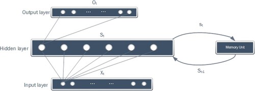
The structure of RNN is illustrated in Figure 1 (Cho et al., 2014).

Figure 1. Recurrent neural networks introduce memory units to record sequence information.

2.6. Finding critical nodes through deep reinforcement learning

The rise of deep learning and reinforcement learning algorithms has led to diverse solutions to many traditional problems, and this is also the case for the CN problem. S2V-DQN makes such an attempt to solve the Critical Nodes problem by combining reinforcement learning with graph embeddings. S2V-DQN uses a greedy strategy to continuously optimise the solution, while continuously enhancing the generalisation performance of the model (Dai et al., 2017). FINDER is improved on the basis of S2V-dqn algorithm, that is, by changing the combination mode of network characteristics and loss function to improve the speed of model convergence and the quality of optimisation strategy (Fan et al., 2020).

3. Method

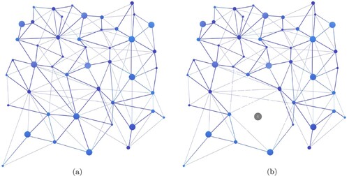
Our approach is to find an optimal critical node removal strategy that minimises the connectivity of the target network with minimal overhead. Firstly, the feature extraction has to be fulfilled.VNS uses the Graph embedding method to complete the information reduction of the target network; then, it uses the DQN method to complete the learning of the optimal policy. Figure 2(a) shows a network structure. In Figure 2(b), node 1 is dismantled, then the connectivity of the network will be changed and all points connected to node 1 will be de-connected from it. If the diagram represents an infectious disease transmission network, node 1 can be considered as a super-infector. If the super-infector can be isolated in time, the number of people infected by the infectious agent will be greatly reduced.

Figure 2. Figure (a) is an original network and Figure (b) is the result after node 1 has been removed. When node 1 is removed from the graph, the connectivity of the graph is changed.

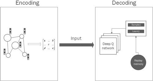
The method in this paper is divided into two main parts, encoding and decoding. The main task in the Encoding part is to embed the features and other information of the target network using the Graph Embeddding method to obtain a low-dimensional representation of the information; the Decoding phase will use the DQN algorithm to perform the vital node search and generate the optimal policy. The model structure of this paper is shown in Figure 3.

Figure 3. In the Encoding section, the feature information of the target network is embeded and then becomes the feature vector input to the decoding section. In the decoding section, DQN will start to explore the optimal strategy.

3.1. Encoding

In this phase, the main implementation is through the GCN method in Graph embedding. More specifically, the method used is the GraphSAGE in GCN. In the GraphSAGE method, the feature vector of the target node is generated by aggregating the neighbouring nodes. During the aggregation, the neighbouring embeddings and self-embeddings of the target node are stitched together by the concat operation. After several cycles of aggregation, the final form of the node feature vector will be obtained. The algorithm for Encoding is described as below:

In Algorithm 1, we first initialise the embedding vector $h_v^{(0)}$. Then we will input a Graph $G(V,E)$ and the feature matrix $X_v$ and update $h_v^{(0)}$ according to the neighbours features of the target node by K times sampling.

3.2. Decoding

In this phase, we use the DQN algorithm to complete the generation of the optimal target strategy. The reason for using DQN is mainly due to the following considerations.

• traditional algorithms for finding vital nodes are usually proposed for a particular problem and are not generalisable;

• machine learning methods have strong generalisation properties, and training with large amounts of training data can help the model improve its ability to solve real-world problems;

• DQN algorithms, a major innovation in the field of machine learning at present, combine the advantages of reinforcement learning and deep learning and can massively reduce the time and space scale of the problem.

It should be noted that although the traditional DQN model has many advantages, it still has some drawbacks, especially for the vital node finding problem discussed in this paper. Firstly, in the traditional DQN model, $Q(s,a)$ represents the value of executing a under state s. When both state s and action a determine the value of Q, $Q(s,a)$ does not fully represent the value of state a, since there may be some state that has no significant effect on the state at the next t moments, regardless of any action performed by the agent. Consider the following possibilities: in a particular state, the agent gets a higher value regardless of any action it performs; in another state, the agent chooses any action and only gets a lower value. Second, finding critical nodes should consider sequential information. At moment t, the agent performs a node removal operation on the target network, which will necessarily affect the connectivity of the residual graph. When moving to the operation at moment t + 1, the agent should consider the information at moment t. Traditional deep neural networks only consider the influence of the previous input and not the other inputs, so we introduce the LSTM network to inherit the information from the previous moment, that is, not only consider the previous input, but also give the network a memory of the previous content.

Therefore, in contrast to the traditional DQN, we have modified the network structure with the following changes:

1. adding LSTM networks to enable processing sequential information;

2. dividing the last fully connected layer of the traditional DQN into two branches, and then merging the results of the two branches to generate the predicted Q values.

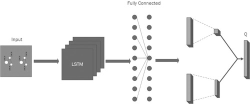
More specifically, the upper branch of the two branches in the Q Network produces an advantage value and the lower branch produces the value corresponding to the action, and these two values are added together to obtain the final Q value of the action The model structure of the DQN network is shown in Figure 4 below.

Figure 4. An LSTM layer is added to the DQN and the last layer of the fully connected network is split into two in for merging and finally generating Q values.

The algorithm for decoding is described as follows.

The input data $z_v$ in Algorithm 2 is the output of Algorithm 1. In Algorithm 2, we first process $z_v$ with the LSTM layer, and then initialise the Q network and the experience replay buffer. The next step is the calculation of Q values. In the third line of Algorithm 2, $z_v$ is first multiplied with two weight matrices $W_2$ and $W_3$, then passes through the ReLU layer, and finally multiplies by a weight matrix $W_1^T$ to get the Q value. After N episodes, the Q value is continuously updated and approximates the target Q value.

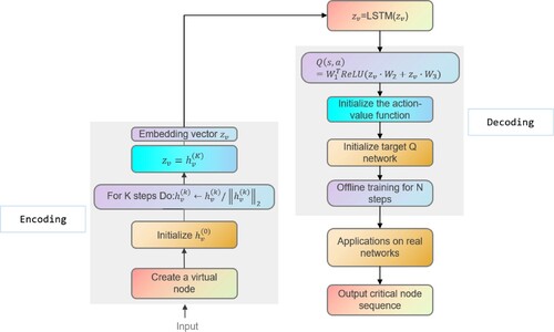
The flow chart of the algorithm is shown in Figure 5:

Figure 5. The left side is the encoding phase and the right side is the decoding phase. The final output is the sequence of critical nodes.

Algorithm 1 obtains the embedding vector $z_v$ of the target network. $z_v$ is used as the input of the Decoding stage. As mentioned above, traditional DQN has many problems that lead to large deviations in the predicted Q values, and the robustness of DQN decreases in the face of insufficient information. Therefore, Algorithm 2 improves on these two drawbacks. First, $z_v$ is passed into the LSTM network layer to obtain the output result after LSTM processing, at which time the value of $z_v$ is updated; then, the Q network and the target Q network are initialised. In order to reduce the error between the predicted Q value and the real Q value, we add the value network layer and the dominance network layer, as shown in Figure 7. The value network layer considers only state S, and the dominance network layer considers both state S and action A. The output of the final Q network is obtained by linearly combining the output of the price function network and the output of the dominance function network.

For example, we use the Crime dataset to verify the effectiveness of the algorithm. First, VNS obtains the embedding vector of the Crime dataset and then decodes it. in the decoding phase, VNS feeds the embedding vector of the Crime dataset to the LSTM layer to obtain a new matrix output. This way of processing will retain more sequence information. Entering the Doceding phase, when obtaining the Q values, VNS replaces the original Q values with a linear combination of the output values from the Value network layer and the Advantage network layer. Compared with the FINDER model, the ANC score obtained by VNS on the Crime data set is lower. The architecture of VNS is shown in Figure 6.

Figure 6. The architecture diagram of VNS. The features of the target graph will be processed by Graph embedding and LSTM respectively, and then pass through a layer of fully connected layers to finally obtain the output vector; finally, it will be decoded by DQN.

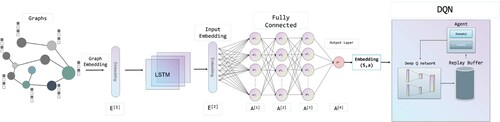
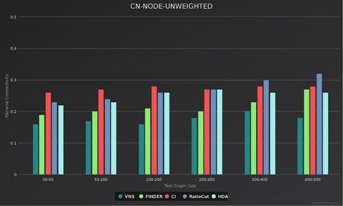
Figure 7. Green represents VNS, purple represents FINDER, blue represents CI, yellow represents RatioCut and red represents HDA. These synthetic graphs have 30–50, 50–100, 100–200, 200–300, 300–400 and 400–500 nodes, respectively, and the nodes have no weights. The Y-axis represents the pairwise connectivity, and the X-axis is the size of the test graph.

In the training phase, first we use the generated virtual graph to train the VNS model. In each episode, VNS will continue to find all potential critical nodes on the given graphs until it reaches the final state. During training, a state-action sequence $(s_0,a_0,r_0,s_1,r_1,s_2,\dots ,s_T)$is generated. VNS defines a control function to complete the entire episode, which includes generating trajectories and storing them in the experience replay buffer. During training, we use the e-greedy policy with linearly annealing from 1.0 to 0.05 over the 10,000 episodes to balance between exploration and exploitation. After training for up to a million episodes, the e will eventually drop to 0.05 and remain stable, at which point we consider the model to have completed its exploration and reached a state of convergence. Every 300 episodes, we evaluate the performance of the agent and randomly sample small batches of 4-tuple trajectories in each episode for stochastic gradient descent updates to minimise the loss function.

3.3. Complexity analysis

Because the algorithm of VNS model is divided into encoding phase and decoding phase, the complexity of the algorithm of VNS model will be calculated respectively. First is the complexity analysis of the encoding phase. As shown in algorithm $S1$, the encoding complexity is A, where K is the number of propagation steps, which is usually a constant less than 10; N is the number of network nodes; and N is the average number of neighbours of the nodes. Because the matrix product is used in algorithm $s1$, the complexity of the encoding phase is $O(E)$, where E is the number of edges and the dimension of the adjacency matrix. Then comes the complexity analysis of the decoding phase. Since the main task of the decoding phase is to obtain the mapping of state-action pairs to the scalar value $Q(s,a)$, we implement this mapping relationship using the following equation: (6) $Q(s,a)={W_1}^T\mathrm{Re}LU(z_{\mathrm{LSTM}}\cdot W_2+z_{\mathrm{LSTM}}\cdot W_3)$(6) where $W_1,W_2$ and $W_3$ are the weight matrices and $z_{\mathrm{LSTM}}$ is the vector obtained from the output of Algorithm ?? after further processing by the LSTM layer. Thus to compute the Q values of all nodes, the time complexity is $O(N)$. The last comes from the greedy selection step. Since we use the batch nodes selection strategy to select the first n nodes with the highest Q value each time, the time complexity is $O(N\log N)$. In summary, the total time complexity of VNS should be $O(E+N+N\log N)$.

3.4. Solve curse of dimensionality with function approximation

Curse of Dimensionality is a phenomenon that occurs in machine learning when the computation of vectors increases exponentially due to the increase in dimensionality. VNS takes an effective approach to avoid it in both encoding and decoding phases. In the encoding phase, we map the input graph to a low-dimensional space by Graph embedding and encode the action a and state s into an embedding vector. Traditional reinforcement learning methods (Q-learning) use Q-table to compute a large number of Q values and thus lead to dimensional disasters, so in the decoding phase, we use Function Approximation instead of Q tables, which can reduce the complexity of computation and decrease the computational effort.

4. Results and analysis

4.1. Experimental settings

We compared VNS with traditional methods on real datasets. We used the Barabási-Albert (BA) model to generate virtual networks with nodes in the range 30–500 for training the VNS model, and then validated it on the real dataset. Four real-world network datasets were selected, namely Crime, HI-II-14, Digg and Enron.

Crime (Kunegis, 2013): The Crime dataset is a mapping of offenders to crime relationships. Each node represents a terrorist and each edge represents a link between terrorists.

HI-II-14:¹ The HI-II-14 dataset is a mapping of protein and protein-protein interactions. Each node represents a protein and each edge represents an interaction between proteins.

Digg (Kunegis, 2013): The Digg dataset is a mapping network of comment relationships in the social networking site Digg. Each node represents a user of the Digg website and each edge represents the existence of a comment relationship between two users.

Enron (Leskovec et al., 2008): The Enron dataset is a mapping of email contact networks. Each node represents an email address and each edge represents the existence of at least one email contact between email addresses.

4.2. Evaluation metrics

First we need to define appropriate metrics to quantify network functionality. For most network-based applications, they run in a connected environment, so network connectivity can be an important proxy for network functionality. Commonly used network connectivity metrics include the number of connected components, pairwise connectivity, the size of the giant connected component (GCC), accumulated normalised In fact, the optimal attack problem with the goal of minimising ANC socre is exactly equivalent to the optimal propagation problem with linear threshold propagation dynamics (Morone & Makse, 2015).

In order to further compare the performance of the model, in addition to ANC, Time Consumption, we introduced pairwise connectivity: (7) ${\sigma }_{pair}(G)=\sum _{C_i\in G}\frac{{\delta }_i({\delta }_i-1)}{2}$(7) where $C_i$ is the $i\mathrm{th}$ connected component in the current graph G, and ${\delta }_i$ is the size of $C_i$.

Therefore, we will use ANC score on real world networks (Fan et al., 2020), pairwise connectivity on synthetic networks (Arulselvan et al., 2009), pairwise connectivity of residual graph and test consumption time as evaluation metrics of model performance (Fan et al., 2020). Different models are experimented on the same dataset and a lower ANC score indicates a higher performance of than other models. We will also compare the time demand of different models on the same dataset.

4.3. Results

The procedure of the experiments was as follows: first, we trained the VNS model using a randomly generated Synthetic network. The network used for training was a miniature network with no more than 500 nodes allowing to quickly improve the generalisation of the model; once the training process was completed, the model was tested with synthetic graphs and real datasets. It should be noted that the datasets used for the experiments were Crime, HII-II-14, Digg and Enron, which contain 829, 4165, 29,652 and 33,969 nodes respectively and are basically representative of real-world network data.Synthetic graphs are generated by the BA model and the number of nodes varies from 30 to 500.

Results on synthetic graphs. To verify the performance of the VNS, we firstly tested it on synthetic graphs. These synthetic graphs have 30–50, 50–100, 100–200, 200–300, 300–400 and 400–500 nodes, respectively, and the nodes have no weights. For each node size,we generated 100 graphs at random and averaged the results from all trials.

We use pairwise connectivity to measure the results of each model running on the same synthetic graph (Fan et al., 2020). From Figure 7, we can learn that the pairwise connectivity scores of VNS are all the lowest when the number of nodes of the generative graph is 30–50, 50–100, 100–200, 200–300, 300–400, 400–500, respectively, with 0.16, 0.17, 0.16, 0.18, 0.20, 0.18, which are at least 16%, 15%, 24%, 10%, 13% and 33% lower than the remaining four models, respectively. This means that VNS is able to find the optimal sequence of vital nodes that allows it to maximise the change in network connectivity on all sizes of graphs.

Results on real-world graphs. The experimental results are shown as follows. Figure 8 shows the ANC scores of different models on the same dataset (the lower the score, the higher the performance). Figures 9–12 shows the ANC curves of different models on the Crime, HII-II-14, Digg and Enron datasets.

Figure 8. ANC scores for the models HDA, CI, RatioCut, FINDER and VNS tested on the real datasets Crime, HI-II-14, Digg, Enron.

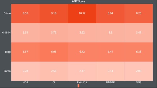
Figure 9. ANC curves for different models on the Crime dataset. There are 829 nodes in the Crime dataset, so the ANC curve has a dashed shape.

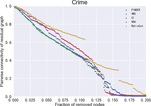
Figure 10. ANC curves for different models on the HI-II-14 dataset. There are 4165 nodes in the HI-II-14 dataset, so the ANC curve is more continuous.

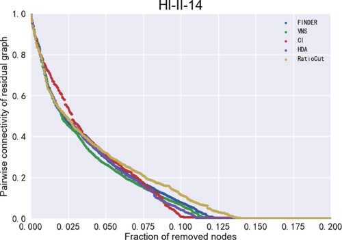
Figure 11. ANC curves for different models on the Digg dataset. There are 29,652 nodes in the HI-II-14 dataset, so the ANC curve is very continuous.

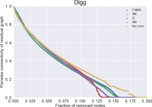
Figure 12. ANC curves for different models on the Enron dataset. There are 33,696 nodes in the Enron dataset, so the ANC curve is the most continuous.

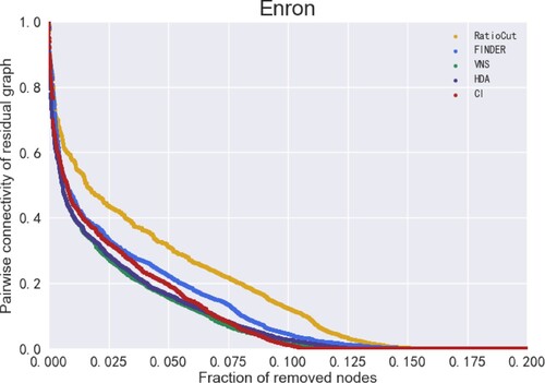
The x-axis in Figures 9–12 represents the size of the removed nodes and the y-axis represents the pairwise connectivity value of the residual graph (Fan et al., 2020). the smaller the value of pairwise connectivity, the smaller the connectivity of the residual graph, which means that the model is more capable of finding vital nodes. It can be seen that the VNS model in this paper performs best on the Crime, HII-II-14, Digg and Enron datasets, indicating the VNS model performs best on finding vital nodes to find vital nodes. More specifically, removing nodes of the same size enables VNS to make the lowest pairwise connectivity of the residual graph compared to the remaining four models, which also means that the sequence of vital nodes found by VNS has the greatest impact on the connectivity of the network. In other words, VNS is the most efficient and effective in finding vital nodes.

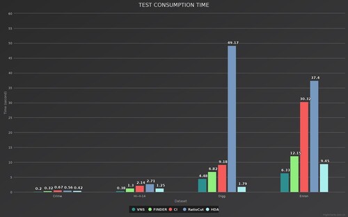
Time consumption is also a key factor in measuring the performance of the model in finding vital nodes. Figure 13 shows the time taken by the different models when testing the dataset. As the size of the dataset increases exponentially, the consumed time increases significantly. It can be concluded that VNS consumes least amount of time. The results show that the time consumed by VNS in four datasets, Crime, HI-II-14, Digg, and Enron, is at least 38%, 70%, 34%, and 33% lower than the remaining four models, respectively.

Figure 13. Test time requriements for different models on the datasets.

4.4. Comprehensive analysis

To verify the ability of the model to solve the vital node problem, four metrics were chosen for comparison: ANC score on real world networks, pairwise connectivity of residual graph, pairwise connectivity on synthetic networks, and Test Consumption time. The experimental results showed that VNS outperformed the other models in all four metrics. In particular, as shown in Table 1, the values of ANC score for VNS on the Crime, HI-II-14, Digg and Enron datasets are lower than the remaining four models (lower ANC score means lower connectivity of the network, then better performance). Figures 9–12 shows that after removing nodes of the same size, the residual graphs processed by VNS has the lowest pairwise connectivity. Figure 13 indicates the performance of VNS on synthetic graphs, and it is clear that VNS performs best on generative graphs of all sizes. Finally, we compared the time taken by different models to complete the task on the same dataset. The results show that VNS consumes the least amount of time and performs the best (Figure 14).

Figure 14. The mean Time Consumption values for the different models on the four datasets and the mean ANC Score. Where cyan represents the Time Consumption of each model and purple represents the ANC Score.

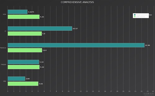
Table 1. The ANC scores for the models HDA, CI, RatioCut, FINDER and VNS tested on the real datasets Crime, HI-II-14, Digg, Enron.

Dataset	HDA	CI	RatioCut	FINDER	VNS
Crime	8.52	9.18	10.32	8.84	8.25
HI-II-14	3.51	3.72	3.62	3.50	3.42
Digg	6.57	6.95	6.42	6.41	6.38
Enron	2.24	2.56	2.17	2.14	2.03

4.5. Industrial significance

vital nodes are used in practice in a wide range of industrial areas such as risk management, network vulnerability assessment, biomolecular research, drug synthesis, protein network analysis, social network analysis and many more. VNS can be used in industry to minimise the time and space costs and to improve the speed of finding vital nodes. More importantly, VNS is a highly flexible framework, which means that VNS can be used in a wide range of applications. VNS may play such roles in industry:

1. the search for key targets in drug manufacturing;

2. the identification of key proteins in PPI;

3. the search for maximum congestion points in traffic networks;

4. the determination of the best drop-off points for public transportation.

5. Conclusion

In summary, VNS excels in solving the vital node problem of complex networks, outperforming other models in terms of efficiency and effectiveness. This approach opens up a new direction for optimising vital node models: (1) enhancing the performance of the model with more methods that can be applied to optimise deep learning network models. (2) improving the robustness of the model in the face of insufficient information and greatly improving the generalisation of the model. In addition, VNS can be applied in several industrial fields to help us design more robust networks.

There may be some possible limitations in this study. The graph embedding method of VNS is more time consuming and space consuming and less efficient on large networks. This is mainly due to the neighbour explosion phenomenon: GNN will continuously aggregate the information of neighbouring nodes in the graph, then each target node in the L-layer GNN needs to aggregate the information of all nodes within the L-hop in the original graph. In a large graph, the number of neighbouring nodes can grow exponentially with L.

Disclosure statement

In accordance with Taylor & Francis policy and our ethical obligation as researchers, we confirm that there are no relevant financial or non-financial competing interests to report.

Additional information

Funding

This work was supported by National Natural Science Foundation of China [61303108]; Natural Science Foundation of Jiangsu Province [BK20211102]; Suzhou Key Industries Technological Innovation-Prospective Applied Research Project [SYG201804]; A project funded by the Priority Academic Program Development of Jiangsu Higher Education Institutions.

Notes

1 http://interactome.baderlab.org/data/Rolland-Vidal(Cell2014).psi

References

- Arulselvan, A., Commander, C. W., Elefteriadou, L., & Pardalos, P. M. (2009). Detecting critical nodes in sparse graphs. Computers & Operations Research, 36(7), 2193–2200. https://doi.org/10.1016/j.cor.2008.08.016
- Borgatti, S. P. (2006). Identifying sets of key players in a social network. Computational & Mathematical Organization Theory, 12(1), 21–34. https://doi.org/10.1007/s10588-006-7084-x
- Chen, D., & Trivedi, K. S. (2017). Optimization for condition-based maintenance with semi-Markov decision process. Reliability Engineering & System Safety, 90(1), 25–29. https://doi.org/10.1016/j.ress.2004.11.001
- Cho, K., Merrienboer, B. V., Gulcehre, C., Ba Hdanau, D., Bougares, F., Schwenk, H., & Bengio, Y. (2014). Learning phrase representations using RNN encoder-decoder for statistical machine translation. In Proceedings of the 2014 Conference on Empirical Methods in Natural Language Processing (EMNLP).
- Dai, H., Khalil, E. B., Zhang, Y., Dilkina, B., & Song, L. (2017). Learning combinatorial optimization algorithms over graphs.
- Dall'Asta, L., & Braunstein, A. (2016). Network dismantling.
- Fan, C., Zeng, L., Sun, Y., & Liu, Y. Y. (2020). Finding key players in complex networks through deep reinforcement learning. Nat Mach Intell, 2, 317–324. https://doi.org/10.1038/s42256-020-0177-2
- Grover, A., & Leskovec, J. (2016). node2vec: Scalable feature learning for networks. In 22nd ACM SIGKDD international conference. ACM.
- Jaouadi, M., & Romdhane, L. B. (2019). Influence maximization problem in social networks: An overview. In 2019 IEEE/ACS 16th international conference on computer systems and applications (AICCSA). IEEE.
- Kipf, T. N., & Welling, M. (2016). Semi-supervised classification with graph convolutional networks.
- Kunegis, J. (2013). KONECT: The Koblenz network collection. In International conference on world wide web companion. ACM.
- Lalou, M., Tahraoui, M. A., & Kheddouci, H. (2018). The critical node detection problem in networks: A survey. Computer Science Review, 28(1574-0137), 92–117. https://doi.org/10.1016/j.cosrev.2018.02.002
- Leskovec, J., Lang, K. J., Dasgupta, A., & Mahoney, M. W. (2008). Community structure in large networks: Natural cluster sizes and the absence of large well-defined clusters. Internet Mathematics, 6(1), 29–123. https://doi.org/10.1080/15427951.2009.10129177
- Li, A., & Liu, Y. Y. (2020). Controlling network dynamics. Advances in Complex Systems (ACS), 22(07n08), 1950021. https://doi.org/10.1142/S0219525919500218
- Lubeck, M., Kondapalli, N., & Kasaraneni, J. (2012). Network connectivity (U.S. US8175001 B2).
- Maji, G., Dutta, A., Malta, M. C., & Sen, S. (2021). Identifying and ranking super spreaders in real world complex networks without influence overlap. Expert Systems with Applications, 179, 115061. 0957-4174. https://doi.org/10.1016/j.eswa.2021.115061
- Meeravali, S., Bhattacharyya, D., Rao, N. T., & Hu, Y. C. (2021). Performance analysis of an improved forked communication network model. Connection Science, 33(3), 645–673. https://doi.org/10.1080/09540091.2020.1867064
- Mnih, V., Kavukcuoglu, K., Silver, D., Graves, A., Antonoglou, I., Wierstra, D., & Riedmiller, M. (2013). arXiv e-prints.arXiv:1312.5602
- Morone, F., & Makse, H. A. (2015). Corrigendum: Influence maximization in complex networks through optimal percolation. Nature, 524, 65–68. https://doi.org/10.1038/nature14604
- Morone, F., & Makse, H. A. (2015). Influence maximization in complex networks through optimal percolation. Nature, 524(7563), 65–68. https://doi.org/10.1038/nature14604
- Mozer, M. C., Touretzky, D. S., & Hasselmo, M. (2005). Reinforcement learning: An introduction. ieee Transactions on Neural Networks, 16(1), 285–286. https://doi.org/10.1109/TNN.2004.842673
- Mugisha, S., & Zhou, H. J. (2016). Identifying optimal targets of network attack by belief propagation. Physical Review E, 94(1), 012305. https://doi.org/10.1103/PhysRevE.94.012305
- Nazari, M., Oroojlooy, A., Snyder, L. V., & Takáč, M. (2018). Reinforcement learning for solving the vehicle routing problem.
- Perozzi, B., Al-Rfou, R., & Skiena, S. (2014). Deepwalk: online learning of social representations. ACM.
- Qiu, L., Sai, S., & Tian, X. (2021). TsFSIM: A three-step fast selection algorithm for influence maximisation in social network. Connection Science, 33(4), 854–869. https://doi.org/10.1080/09540091.2021.1904206
- Ren, X. L., Gleinig, N., Helbing, D., & Antulov-Fantulin, N. (2018). Generalized network dismantling. Proceedings of the National Academy of Sciences, 116. https://doi.org/10.1073/pnas.1806108116
- Rodriguez-Nunez, E., & Garcia-Palomares, J. C. (2014). Measuring the vulnerability of public transport networks. Journal of Transport Geography, 35(0966-6923), 50–63. https://doi.org/10.1016/j.jtrangeo.2014.01.008
- Sabe, V. T., Ntombela, T., Jhamba, L. A., Maguire, G., & Kruger, H. G. (2021). Current trends in computer aided drug design and a highlight of drugs discovered via computational techniques: A review. European Journal of Medicinal Chemistry, 224, 113705. 0223-5234. https://doi.org/10.1016/j.ejmech.2021.113705
- Schneider, C. M., Moreira, A. A., Jr., Andrade, J., Havlin, S., & Herrmann, H. J. (2011). Mitigation of malicious attacks on networks. Proceedings of the National Academy of Sciences of the United States of America, 108(10), 3838–3841. https://doi.org/10.1073/pnas.1009440108
- Shen, Y., N. P. Nguyen, Ying, X., & Thai, M. T. (2013). On the discovery of critical links and nodes for assessing network vulnerability. IEEE/ACM Transactions on Networking, 21(3), 963–973. https://doi.org/10.1109/TNET.2012.2215882
- Tang, J., Qu, M., Wang, M., Zhang, M., Yan, J., & Mei, Q. (2015). Line: Large-scale information network embedding. In International conference on world wide web (WWW).International World Wide Web Conferences Steering Committee
- Wu, S., Liu, Y., Zou, Z., & Weng, T. H. (2022). S_I_LSTM: Stock price prediction based on multiple data sources and sentiment analysis. Connection Science, 34(1), 44–62. https://doi.org/10.1080/09540091.2021.1940101
- Xu, D., Ruan, C., Korpeoglu, E., Kumar, S., & Achan, K. (2020). Inductive representation learning on temporal graphs.
- Yan, S., Xu, D., Zhang, B., Zhang, H. J., Yang, Q., & Lin, S. (2007). Graph embedding and extensions: A general framework for dimensionality reduction. IEEE Transactions on Pattern Analysis & Machine Intelligence, 29(1), 40–51. https://doi.org/10.1109/TPAMI.2007.250598
- Zdeborová, L., Zhang, P., & Zhou, H. J. (2016). Fast and simple decycling and dismantling of networks. Scientific Reports, 6(1), 1–6. https://doi.org/10.1038/s41598-016-0001-8
- Zhang, S., Yao, T., Sandor, V. K. A., Weng, T. H., & Su, J. (2021). A novel blockchain-based privacy-preserving framework for online social networks. Connection Science, 33(3), 555–575. https://doi.org/10.1080/09540091.2020.1854181
- Zhu, X., Zuo, J., & Ren, H. (2019). A modified deep neural network enables identification of foliage under complex background. Connection Science, 32(4), 1–15. https://doi.org/10.1080/09540091.2019.1609420