A hybrid optimization method by incorporating adaptive response strategy for Feedforward neural network

Abstract

Particle swarm optimisation algorithm (PSO) possesses a strong exploitation capability due to its fast search speed. It, however, suffers from an early convergence leading to its inability to preserve diversity. An improved particle swarm optimiser is proposed based on a constriction factor and Gravitational Search Algorithm to overcome premature convergence. The constriction factor ensures an appropriately controlled transition from exploration into exploitation, leading to an enhanced diversity and appropriate learning rate adjustment throughout the search process. We introduce Gravitational Search Algorithm to enhance the exploratory ability of PSO. An adaptive response strategy is incorporated to activate stagnated particles to curtail the high tendency to get trapped in a local optimum. To verify the efficacy of the improvement strategies, we employ the proposed algorithm in training a Single Layer Feedforward neural network to classify real-world data ranging from binary to multi-class datasets of which our proposed algorithm outperforms the others.

KEYWORDS:

• Gravitational search algorithm
• particle swarm optimisation
• adaptive response strategy
• Feedforward neural network

1. Introduction

As one of the most implemented Artificial Neural Networks (ANN) architectures, Feedforward neural network (FNN) possesses an excellent ability to learn (Nayak et al., 2018). However, a challenge still exists when FNN is employed to train ANNs (Saremi et al., 2014). The traditional Back-propagation algorithm (B.P) (Jiang and Hu et al., 2019) used to train FNNs have inherent limitations, such as slow convergence, time-consuming, difficulty in adjusting the weights and thresholds, high tendency to fall into a local minimum, and high sensitivity to the choice of learning rate η (Ram & Rao, 2018).

Several researches have proposed variant metaheuristics with fast training speed, good generalisation performance, and a higher likelihood to locate the global optimal solution to overcome the challenges of FNNs (Amponsah et al., 2021; Han et al., 2019; Lalwani, 2021; Šešum-Čavić, 2020). As one of the widely used metaheuristics to effectively train FNNs, Particle swarm optimisation cannot preserve diversity throughout the optimisation process. Hence, this study proposes a hybrid PSO based on Gravitational search algorithm (GSA) and Adaptive response strategy (ARS). The proposed algorithm uses the GSA to enhance exploration, the constriction factor to switch from exploration to exploitation, and the ARS to prevent premature convergence and preserve swarm diversity throughout the optimisation. The resulting hybrid algorithm is called HPSOGSA-ARS. We summarise our contributions as follows:

• An Adaptive Response Strategy (ARS) is incorporated to move stagnated particles in sub-optimal solutions into promising areas.

• A constriction factor comprising a convex and concave function ensures an appropriately controlled transition from exploration into exploitation. The constriction factor enhances diversity, appropriate learning rate adjustment, and increased overall performance by providing a smooth transitioning.

This article is organised as follows. Section 2 discusses previous works related to metaheuristics in optimising FNNs and preliminary information about the constitutive algorithms. We then present the details of the proposed FNN training method in Section 3. The experimental results on implemented UCI datasets, related mechanisms analysis, and running time are given in Section 4. Finally, we offer the concluding remarks in Section 5.

2. Related works

Regarding the training of FNNs, two types of approaches exist: iterative and non-iterative (Suganthan, 2018; Zhang et al., 2021). In the non-iterative neural network training approach, the hidden nodes are randomly selected and maintained throughout the training process, whereas the output weights are computed analytically (Zhang et al., 2020).

Examples of the non-iterative training approaches are as follows: In (Mukherjee et al., 2021), the authors proposed an improved version of the Sine Cosine Algorithm (SCA) called: chaotic oppositional SCA (COSCA) to solve the challenge of premature convergence. They improved the algorithm by integrating chaos theory and oppositional-based learning into the SCA optimisation process. Although the algorithm could obtain the least error by finding the best control parameters to train an FNN, it required much time and computational resources to complete execution. In (Cui et al., 2018), the authors identified the inability of exiting methods to recognise malicious code at an acceptable accuracy and speed. They therefore aimed at solving this challenge by proposing a novel approach that used a convolutional neural network (CNN) and a bat algorithm to automatically extract the features of malware images and address the data imbalance among different malware families. Although their proposed model achieved a good accuracy and speed, it requires all input images to have a fixed size resulting in limited scalability. Similar to (Yi et al., 2016), the authors of (Wang et al., 2016) successfully improved the Single Layer Feedforward Neural Network Extreme Learning Machine (SLFNELM) by proposing a self-adaptive mechanism that solved the limitation of SLFNELM being sensitive to the number of neurons within its hidden layer. The resulting algorithm was named: SaELM. SaELM can select the best neuron number in the hidden layer to construct an optimal Neural Network. A series of experiments confirmed SaELM to be a fast-training method capable of obtaining the global optimal solution with a good generalisation performance independent of parameter adjustments.

On the other hand, the iterative technique aims to fine-tune the weights and bias of the Feedforward neural network together with its structure until an ideal result is achieved (Sugiyama et al., 2021). Some examples of the iterative training approach are as follows: Derivative-based learning strategies generally have high computational costs due to the large number of weight values that require tuning (Eyoh et al., 2020). In (Sağ & Jalil, 2021), the authors aimed at solving the difficulty of derivative learning-based strategies by implementing the Vortex Search (VS) algorithm to determine the optimal weights and biases of the FNN. Although the authors achieved the research objective, the algorithm has a limitation regarding generalisation performance. Again, (Yang & Ma, 2019) proposed a dictionary learning approach based on the singular value decomposition (SVD). The SVD creates a compact structure of an FNN by selecting significant hidden neurons depending on their contribution to outputs. Although this algorithm could simultaneously train the FNN and optimise its network, it introduced more hidden neurons, increasing computational time and resources. In (Wang et al., 2013), the authors proposed a mother function selection algorithm that improved the accuracy and usefulness of wavelets for target threat assessment in aerial combat. Although the algorithm could construct an enhanced Neural Network with a better mean square error (MSE) value via selecting the most appropriate wavelet function, the number of functions alternatives from which the selection algorithm chose was limited to seven.

Although the iterative approach produced a superior result to the non-iterative method in most cases, it is typically computationally intensive and time-consuming (Karamichailidou et al., 2021). Therefore, researchers mostly employ the non-iterative approach by incorporating metaheuristics such as fireworks algorithm (Konda et al., 2021; Sreeja, 2019), Particle Swarm Optimisation (PSO)(Nagra et al., 2019; Neshat et al., 2020; Zemmal et al., 2021), Genetic Algorithm(G.A.) (Christo et al., 2020; Falahiazar & Shah-Hosseini, 2018), firefly algorithm (Liu et al., 2021), Gravitational Search Algorithm (GSA) (Bohat & Arya, 2018; Huang et al., 2019) with improvement strategies to enhance training performance. Similar works of this nature include the following:

The authors Amponsah et al. (Amponsah et al., 2021) proposed an improved multi-leader comprehensive learning particle swarm optimiser based on Karush-Kuhn-Tucker proximity measure and Gravitational Search Algorithm. This improvement was implemented to overcome the limitation of the multi-leader comprehensive learning particle swarm optimiser in preserving diversity. The proposed algorithm outperformed other state-of-the-art FNN training algorithms used to train a Feedforward neural network for epilepsy detection. Similarly, Lei et al. proposed an aggregate learning gravitational search Algorithm (ALGSA) to improve GSA’s exploitation ability during the later stages of iterations when the value of $G$ (the gravitational constant) is sufficiently large. ALGSA used $Kbest$ individuals to construct different gravitational fields which attracted other search agents at the later stages of iteration (Lei et al., 2020). Even though the authors achieved their research objective, this achievement came at the cost of high computation and sensitivity to the learning rate $\eta$.

Furthermore, (Rather et al., 2021) proposed a novel hybrid chaotic gravitational search algorithm (CGSA) and particle swarm optimisation (PSO) to train a multi-layer perceptron (MLP) neural network for classification purposes. Although this unique hybridisation method produced highly accurate classification outcomes, the inherent challenge of local minima entrapment prevailed during the later stages of the search. The motivation of this work is to develop yet another hybrid variant of PSOGSA that alleviates the limitations mentioned above. We seek to achieve this aim by preserving diversity, kerbing the challenge of local optima stagnation, and ensuring a proper balance in learning rate adjustment during the entire optimisation process.

2.1. Particle swarm optimisation (PSO)

Particle swarm optimisation (PSO) is a population-based stochastic optimisation algorithm developed by Eberhart and Kennedy (Russell & James, 1995). A randomly initialised group of birds initiates the mechanism of the PSO in a search landscape. Each of the birds denotes a particle. Each of the particles moves at a velocity influenced by the momentum, its prior best position $(P_{id})$ and the best position of all particles $(P_{gd})$. Supposing the search space is $D$ and the sum of particles is $n$, PSO can be mathematically expressed as: (1) $\begin{array}{rl}{v}_{id}(t+1)& =v_{id}(t)+c_1\ast rand()\ast [P_{id}(t)-x_{id}(t)]+c_2\ast rand()\ast [P_{gd}(t)-x_{id}(t)]\end{array}$(1) (2) $\begin{array}{rl}{x}_{id}(t+1)& =x_{id}(t)+v_{id}(t+1)1\le i\le n,1\le d\le D\end{array}$(2) where $v_{id}(t)$ and $x_{id}(t)$ denotes the velocity vector and the position of the $ith$ particle respectively. In the $t-th$ iteration; $P_{id}$ and $P_{gd}$ denotes the best position of the $ith$ particle and the best position of all particles, respectively. $c_{1}and{c}_2$ denotes the acceleration constants, and $rand()$ indicates a random value within the interval of [0,1].

To improve the converging ability of the original PSO, Shi and Eberhart (Xiaohui & Eberhart, 2002; Yuhui & Eberhart, 1998) proposed an adaptive PSO that incorporated an inertia weight into the velocity equation of PSO. We present the improved PSO mathematically as: (3) $\begin{array}{r}{v}_{id}(t+1)=w(t)\ast v_{id}(t)+c_1\ast rand()\ast [P_{id}(t)-x_{id}(t)]+c_2\ast rand()\ast [P_{gd}(t)-x_{id}(t)]\end{array}$(3) $w$ denotes the inertial weight within [$0\le w\le 1$]. Shi and Eberhart further implemented the linearly diminishing technique to adapt the inertia weight as shown below (Xiaohui & Eberhart, 2002): (4) $\begin{array}{r}w(t)=w_{ini}-\frac{(w_{ini}-w_{end})}{T_{max}}\ast t\end{array}$(4) where “$t$” denotes the current iteration value; $w_{ini},w_{end},T_{max}$ denotes the starting inertia weight, the ending inertia weight, and the maximum number of iterations, respectively.

2.2. Gravitational search algorithm (GSA)

The gravitational search algorithm (GSA) proposed by Rashedi et al. is an exploratory optimisation algorithm motivated primarily by the mass-gravity concept. There are four requirements for any mass in GSA: position, inertia mass, passive and active gravitational masses. The position of a mass corresponds to the problem’s solution, and the fitness function determines its gravitational and inertial masses (Rashedi et al., 2010). Given an optimisation problem that uses “$m$” decision variables and an objective function “$fobj,$” each variable has an upper $(ub)$ and a lower ($lb$) limit. The search landscape with “$m$” dimension is bounded by variable “$d‘‘$ as: (5) $\begin{array}{r}{x}^d=x^d\ast (ub-lb)+lb,d=1,2,3,\dots ,m\end{array}$(5)

Considering a system of $N$ masses, the position of the “$ith$” mass is defined by Equation (6) as follows: (6) $\begin{array}{r}{X}_i=(x_i^1,\dots ,x_i^d,\dots ,x_i^m),i=1,2,3,\dots ,N\end{array}$(6) “$x_i^{d^{\prime }}$: The position of the $ith$ mass in the $d^{th}$ dimension.

Equation (7) shows the relationship between the active, inertia, passive masses, and the objective function. The greater the objective function, the higher the value of the mass. (7) $\begin{array}{r}{M}_{ai}(t),M_{ii}(t),M_{pi}(t)\propto fo{b}_{ji}(t)\end{array}$(7) $M_{ai}(t),M_{ii}(t),M_{pi}(t):$The active, inertial, and passive masses, respectively. “$fo{b}_{ji}(t)$” is the objective function of agent “$i$” at time (t).

The aggregate force from the set of denser bodies acting on mass ${}^{\mathrm{\prime }}{i}^{\mathrm{\prime }}$ from mass ${}^{\mathrm{\prime }}{j}^{\mathrm{\prime }}$ at time ${}^{\mathrm{\prime }}{t}^{\mathrm{\prime }}$ is defined by Equation (8). We compute mass $i^{\mathrm{\prime }}s$ acceleration at time $t$ in the $dth$ direction by Equation (9). We use the fitness function in Equation (10) to calculate the masses of agents. Equations (11,12) compute the new velocity and position of a mass, respectively. (8) $F_i^d(t)=\sum _{j\in kbest,j\ne i}ran{d}_i{F}_{ij}^d=\sum _{j\in kbest,j\ne i}ran{d}_{j}G(t)\frac{M_{pi}(t)\ast M_{aj}(t)}{R_{ij}(t)+\epsilon }(x_j^d(t)-x_i^d(t))$(8) (9) $a_i^d(t)=\frac{F_i^d(t)}{M_{ii}(t)},$(9) (11) $v_i^d(t+1)=ran{d}_i\ast v_i^d(t)+a_i^d(t),$(11) (12) $x_i^d(t+1)=x_i^d(t)+v_i^d(t+1)$(12) $M_{aj}$: The active mass gravity relative to mass $j$, $M_{pi}$ denotes the passive mass gravity relative to mass $i$. $G(t)$: denotes the gravitational constant at time $t$. $ran{d}_{i}and$ $ran{d}_j$ are random values within the interval of $[0,1]$, $\epsilon$ is a small positive constant value, the Euclidian gap between masses $i$ and $j$ at time $t$ is denoted by $R_{ij}(t)$.

The gravitational constant, $G$ is initialised on the onset and declines over time as a control mechanism of GSA’s search accuracy. We depict the initial value function with time in Equation (13). (13) $\begin{array}{r}G(t)=G(G_0,t)\end{array}$(13)

GSA’s complex operations are enumerated and shown in (Rashedi et al., 2010).

The two critical features meta-heuristic algorithms use to attain an optimal solution are exploration and exploitation. An algorithm searches locally to converge at the best solution during exploitation, whereas an algorithm explores the entire search landscape during exploration. In PSO, the cognitive component $[P_{id}(t)-x_{id}(t)]$ of the velocity equation, Equation (1) is responsible for exploration, whereas the social component $[P_{gd}(t)-x_{id}(t)]$ ensures exploitation. On the other hand, exploration in GSA is achieved and enhanced by an appropriate selection of random parameter values $(G_{0}and\alpha ),$ whereas exploitation is obtained via the slow movement of heavier agents (Rashedi et al., 2010).

Although the original GSA has a strong exploration ability, the slow movement of denser masses results in a slow search ability during the final iterations as the denser masses limit the convergence of GSA to an optimal solution (Singh et al., 2018). On the contrary, standard PSO performs a faster search with a better exploitation capacity but often cannot adequately explore the search landscape for the optimal global solution. Although merging GSA and PSO on the basis that they complement each other is expected to result in an improved optimisation algorithm, this expected outcome is not always achieved. This variation in expectation is because the resultant algorithm often gets trapped in a local optimum solution during the later iteration stages.

3. The proposed method

3.1. Improved particle swarm optimization

In this section, we improve PSO in three steps, namely:

• Implementing an inertia weight and a constriction factor in a synchronously varying manner.

• Replacing the cognitive component of PSO with the acceleration component of GSA

• Implementing an Adaptive Response Strategy.

3.1.1. Synchronous implementation of an inertia weight and a constriction factor

When we use a constriction factor in PSO’s velocity equation, we do not often use inertia weight in conjunction. The research performed by Lin et al. shows that the PSO algorithm with only a constriction factor $(k)$ as well as the PSO algorithm with only the inertia weight $(w)$ are equivalent in the case of “$k$” being equal to “$w$” (Lin & Yu, 2011). However, the constriction factor $(k)$ and the inertia weight (w) are entirely different. This section addresses the situation where the inertia weight and functional constriction factor are used synchronously.

In the initial search stages of PSO, a particle needs to search within a large range and switch to exploit a limited search space during the later stages to obtain the global optimal solution. Therefore, $k$ must be an enormous value during the early stages and a small value during the later stages. At the same time, $k$ must steadily decrease to the minimum for a more extended period during the final phase of the search (Wei & Xinning, 2010). This shift pattern corresponds to the selection of convex and concave functions based on the value of the constriction factor during different stages of the search. During the early stages of the search, the algorithm relies on the value of the constriction factor to select a convex function which ensures particles find the optimal solution in an extensive range and prevent premature convergence. During the latter stages of the search, the algorithm selects the concave function to slowly adjust the constriction factor to a minimum to ensure an intensified local search. Doing this ensures the smooth convergence of the algorithm toward the global optimum solution. According to the principle mentioned above, the functional constriction factor based on the cosine function is presented in Equation (14) (dos Santos Coelho, 2008).

To prevent premature convergence, (14) $\begin{array}{r}k(t)=\frac{\cos ((\pi /G_{max})\ast T+2.5}{4}\end{array}$(14) “$T$”: Is the number of iterations, $G_{max}=40$ according to the alternating curve of value $k$ as shown in Figure 1.

Figure 1. The altering curve of value.

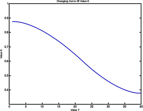
The curve of $k$ in Figure 1 is an alternating curve depicting the synchronous change of the functional constriction factor from a convex function on the onset of the algorithm's execution into a concave function during the later execution stages. Axis “y” (i.e. $k$ values) are the values of the constriction factor, whereas axis “x” (i.e. $T$ values) are the number of iterations.

Incorporating the constriction factor in the standard equation of PSO, Equation (1) results in Equation (15) as follows: (15) $\begin{array}{rl}{v}_{id}(t+1)& =\left(\frac{\cos ((\pi \ast T/G_{max}))+2.5}{4}\right)\\ & \ast [v_{id}(t)+c_1\ast rand()\ast [P_{id}(t)-x_{id}(t)]+c_2\ast rand()\ast [P_{gd}(t)-x_{id}(t)]\end{array}$(15)

When we keep the inertia weight fixed, particles will maintain the same exploratory ability in search. Equation (3) represents a velocity update of the standard PSO with a fixed inertia weight. The foraging process of flocking birds inspires the altering manner of the inertia weight. According to the results of Eberhart et al., the flocking birds slow down to find the precise location of a food source when they get closer to the food source (Russell & James, 1995). If a particle is in a good position in the iterative process, the value of the inertia weight ($w)$ must be decreased to maintain a rigorous exploitation. When the fitness value of a particle is low, “$w$” should be high to retain more of the initial velocity for better global optimisation. Taking into account the research findings of Huang et al. (Huang et al., 2008), Equation (16) shows the exact changes in $‘‘w$”: (16) $\begin{array}{r}\{\begin{array}{ll}w=w_{end}+(w_{start}-w_{end})(1-(T/G_{max}))& if{P}_{gd}\ne x_{id}\\ w=w_{end}& if{P}_{gd}=x_{id}\end{array}.\end{array}$(16)

$T:numberofiterations,T\in [0,G_{max}]$; $P_{gd}$ is the global optimum position; $w_{start}$ is the initial inertia weight and $w_{end}$ is the maximum inertia weight value. We calculate $w_{start}$ and $w_{end}$ as follows:

To facilitate computation, we assume the values of “$k$” and “$w$” to be constants, and we limit our calculation to one dimension. Substituting these constants into Equation (15) results in Equation (17): (17) $\begin{array}{rl}{v}_{id}(t+1)& =k\ast w\ast v_{id}(t)+k\ast c_1\\ & \ast rand()\ast [P_{id}(t)-x_{id}(t)]+k\ast c_2\ast rand()\ast [P_{gd}(t)-x_{id}(t)]\end{array}$(17)

We further calculate the value of $k$ by substituting $c_1\ast rand()$ and $c_2\ast rand()$ with $c_1$ and $c_2$ respectively to obtain Equation (18) as follows: (18) $\begin{array}{r}{v}_{id}(t+1)=k\ast w\ast v_{id}(t)+k\ast c_1\ast [P_{id}-x_{id}(t)]+k\ast c_2\ast [P_{gd}-x_{id}(t)]\end{array}$(18)

Similarly, we obtain $v_{id}(t+2)$ as follows: (19) $\begin{array}{rl}{v}_{id}(t+2)& =k\ast w\ast v_{id}(t+1)+k\ast c_1\ast [P_{id}-x_{id}(t+1)]+k\ast c_2\ast [P_{gd}-x_{id}(t+1)]\end{array}$(19) (20) $\begin{array}{rl}{x}_{id}(t+2)& =x_{id}(t+1)+v_{id}(t+2)\\ & =x_{id}(t+1)+k\ast w\ast v_{id}(t+1)+k\ast c_1\ast [P_{id}-x_{id}(t+1)]\\ & +k\ast c_2\ast [P_{gd}-x_{id}(t+1)]]\\ & =x_{id}(t+1)+kw(x_{id}(t+1)-x_{id}(t))+k{c}_1{P}_{id}-k{c}_1{x}_{id}(t+1)+k{c}_2{P}_{gd}\\ & -k{c}_2{x}_{id}(t+1)\\ & =(1+kw-k{c}_1-k{c}_2)x_{id}(t+1)-kw{x}_{id}(t)+k{c}_1{P}_{id}+k{c}_2{P}_{gd}\end{array}$(20)

The matrix representation of Equation (20), denoted as A, is: (21) $\begin{array}{r}A=\left[\begin{array}{ccc}(1+kw-k{c}_1-k{c}_2)& (-kw)& (k{c}_1{P}_{id}+k{c}_2{P}_{gd})\\ 1& 0& 0\\ 0& 0& 1\end{array}\right]\end{array}$(21)

The homogeneous matrix of Equation (20) is: (22) $\begin{array}{r}\left[\begin{array}{c}{x}_{id}(t+2)\\ x_{id}(t+1)\\ 1\end{array}\right]=A\left[\begin{array}{c}{x}_{id}(t+2)\\ x_{id}(t)\\ 1\end{array}\right]\end{array}$(22)

The characteristic equation of the coefficient matrix for Equation (20) is given by: (23) $\begin{array}{r}(\lambda -1)({\lambda }^2-(1+kw-k{c}_1-k{c}_2)\lambda +kw)=0\end{array}$(23)

From Equation (22), we obtain three characteristic roots as shown below: (24) $\begin{array}{r}\{\begin{array}{c}\lambda =1\\ \alpha ={\displaystyle \frac{1+kw-k{c}_1-k{c}_2+\sqrt{{(1+kw-k{c}_1-k{c}_2)}^2-4kw}}{2}}\\ \beta ={\displaystyle \frac{1+kw-k{c}_1-k{c}_2-\sqrt{{(1+kw-k{c}_1-k{c}_2)}^2-4kw}}{2}}\end{array}\end{array}$(24)

If $(1+kw-k{c}_1-k{c}_2{)}^2\ge 4kw,\alpha$, and $\beta$ are real roots.

If $(1+kw-k{c}_1-k{c}_2{)}^2<4kw,\alpha$, and $\beta$ are imaginary roots. Therefore, when $\alpha$ and $\beta$ are real roots, $\alpha$ and $\beta$ are absolute values else $\alpha$ and $\beta$ are models. For $max(\alpha ,\beta )\le 1$, according to Liu et al. (Liu et al., 2006), we obtain these inequalities: (25) $\begin{array}{r}\{\begin{array}{c}\left|{\displaystyle \frac{1+kw-k{c}_1-k{c}_2+\sqrt{{(1+kw-k{c}_1-k{c}_2)}^2-4kw}}{2}}\right|\le 1\\ \left|{\displaystyle \frac{1+kw-k{c}_1-k{c}_2-\sqrt{{(1+kw-k{c}_1-k{c}_2)}^2-4kw}}{2}}\right|\le 1\end{array}\end{array}$(25)

We obtain inequality (26) after solving inequality (25) as follows: (26) $\begin{array}{r}w\ge \frac{c_1+c_2}{2}-\frac{1}{k}\end{array}$(26)

Since the expression on the right-hand side of the inequality (26) is not a constant, it alters with a change in iterations. Based on the inequality (26), the maximum expression value on the right-hand side evaluates to be equal to or greater than $w$. We can observe from Equation (14) that, when $T$ is 0, $-1/k$ is the maximum value, which is specifically:$-1/((\cos ((\pi /G_{max}\ast 0)+2.5/4))$. From inequality (26), $w_{end}=((c_1+c_2)/2)-1/(\cos ((\pi /G_{max}\ast 0)+2.5/4).$ If $c_1=c_2=2,$ $w_{end}=2-(1/(3.5/4))=\mathrm{0.857143.}$ As $w$ varies from [0, 1], $w_{start}$ is set to $1$. The resulting velocity update equation of PSO after incorporating $w_{start}$ and $w_{end}$ into Equation (3) becomes: (27) $\begin{array}{rl}{v}_{id}(t+1)& =w(t)\ast v_{id}(t)+2\ast rand()\ast [P_{id}(t)-x_{id}(t)]+2\ast rand()\ast [P_{gd}(t)-x_{id}(t)]\\ & \{\begin{array}{l}w=0.857143+(1-0.857143)(1-(T/G_{max}))if{P}_{gd}\ne x_{id}\\ w=0.857143if{P}_{gd}=x_{id}\end{array}\end{array}$(27)

Substituting both the constriction factor and the inertia weight gives a resulting equation: (28) $\begin{array}{rl}{v}_{id}(t+1)& =\left(\frac{\cos ((\pi \ast T/G_{max})+2.5}{4}\right)\\ & \ast [w\ast v_{id}(t)+2\ast rand()\ast [P_{bd}(t)-x_{id}(t)]+2\ast rand()\ast [P_{gd}(t)-x_{id}(t)]]\\ & \{\begin{array}{ll}w=0.857143+(1-0.857143)(1-(T/G_{max}))& if{P}_{gd}\ne x_{id}\\ w=0.857143& if{P}_{gd}=x_{id}\end{array}\end{array}$(28)

3.1.2. Replacement of PSO’s cognitive component with GSA’s acceleration component

This section further enhances PSO’s global exploratory capacity by replacing PSO’s cognitive component with GSA’s acceleration component responsible for global exploration. Using the resulting velocity update equation of PSO in Equation (28), the resulting velocity update equation of the hybrid PSOGSA is as follows: (29) $\begin{array}{rl}{v}_{id}(t+1)& =\left(\frac{\cos ((\pi /G_{max})\ast T+2.5}{4}\right)\\ & \ast [w\ast v_{id}(t)+c_1\ast rand()\ast a_i^d(t)+c_2\ast rand()\ast [P_{gd}(t)-x_{id}(t)]\end{array}$(29) where $v_i^d(t)$ indicates the velocity of agent “i” at iteration “$t$” in the “$dth$” dimension, $c_1=c_2=2$ are acceleration constants, $\omega =\text{inertia weight}$, $rand()$ is any random number within $[0,1],a_i^d(t)$ is the acceleration of agent $\text{ ``}i$” at iteration “$t$” in the “$dth$” dimension and $P_{gd}$ denotes the global best position obtained by all particles.

3.1.3. The adaptive response strategy

In this section, we work on diminishing the tendency of a particle to be trapped in a sub-optimal location while searching for the global optimum solution. We seek to achieve this aim by developing and implementing an adaptive response strategy (ARS). ARS enables particles entrapped in sub-optimal regions to escape entrapment by adjusting their orientation to resume their search for the global optimum solution.

As the algorithm searches for the global optimum solution, diversity is easily lost and can thus get entrapped in a sub-optimal solution. We begin the process of helping trapped particles escape from sub-optimal solutions by observing the $Gbest$ value in any iteration to determine whether it remains unchanged or changed. If the global best fitness value remains unchanged after more than three (3) successive iterations, it means that particles have stagnated. As such, we begin a cycle of positioning whereby the Euclidean distances of particles nearest to the stagnated particle are measured. We then determine the average position of the neighbouring particles relative to the stagnated particle and designate that average position as the new position of the stagnated particle. We express ARS mathematically in a unique position update Equation (30) as follows: (30) $\begin{array}{r}\widehat{x_i}=\stackrel{\rightharpoonup }{x_i}+ran{d}_i\left(1/|N_i|\sum _{n\in N_i}\stackrel{\rightharpoonup }{x_n}\right)\end{array}$(30) where $\widehat{x_i}$ embodies ${x_i}^{\rightharpoonup }$: which is the particle’s new position after the Adaptive Response Strategy (ARS) has taken effect. ${x_i}^{\rightharpoonup }$: indicates the minimum distances from itself comparative to the distances from all the nearest neighbouring particles. The random number $ran{d}_i$: is the actual value within $[-1,1]$. Set $N_i$ holds the indexes of the closest neighbouring particle of a particle ${x_i}^{\rightharpoonup }$. Equation (30) is the new position update equation for stagnated particles.

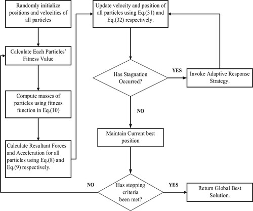
This strategy is an adaptation of a natural phenomenon of flocking birds in finding the ultimate food source and $1/|{\text{N}}_{\text{i}}|\sum _{\text{n}\in {\text{N}}_{\text{i}}}{{\text{x}}_{\text{n}}}^{\rightharpoonup }$: describes the adaptive response of the birds in closest proximity to the bird in the stagnated position relative to the ultimate food source. From old solutions, new solutions emerge after the collaborative behaviour of the flock. Algorithm 1 describes ARS, and Figure 2 is a flowchart representing the entire operations of the proposed algorithm (HPSOGSA-ARS).

Figure 2. General principles of improved hybrid PSO with adaptive response strategy (HPSOGSA-ARS).

As such, we express the improved method mathematically as follows: (31) $\begin{array}{rl}{v}_{id}(t+1)& =\left(\frac{\cos ((\pi /G_{max})\ast T+2.5}{4}\right)\\ & \ast [w\ast v_{id}(t)+c_1\ast rand()\ast [P_{bd}(t)-x_{id}(t)]+c_2\ast rand()\ast [P_{gd}(t)-x_{id}(t)]\end{array}$(31) (32) $\begin{array}{rl}{x}_{id}(t+1)& =x_{id}(t)+v_{id}(t+1)\text{ Else}:\\ x_{id}(t+1)& =\stackrel{\rightharpoonup }{x_i}+ran{d}_i\\ & \times \left(1/|N_i|\sum _{n\in N_i}\stackrel{\rightharpoonup }{x_n}\right)ifgbest[i{]}^t==gbest[i{]}^{t}after3consecutiveiterations.\end{array}$(32)

Algorithm 1. Adaptive Response to Adjust Particles for Minimisation Problem.

Let $N$ denote the number of particles and $Gbest$ also indicate the optimum value;

then the optimal solution will be represented as $Sbest$;

for $i=1:N$

 Identify the nearest seven neighbours with Euclidean distance and preserve the neighbour $(n)$ index in the set $N_k$;

 Compute the new position via Equation (32)

End

$Gbest=$ The least fitness value compared to the fitness values of all other particles;

$Sbest=$ Best solution among $Gbest$ solution obtained from every iterative solution.

3.2. Computation complexity

The complexity of HPSOGSA-ARS comprises four aspects; joint enhanced exploratory search due to implementation of GSA’s acceleration component, Adaptive Response Strategy, and operations of a convex function and a concave function as influenced by the value of the constriction factor. The convergence of the HPSOGSA-ARS is dependent on a progressive update of both the velocity and position equations $v_{id}$ and $x_{id}$, respectively.

Suppose we execute the algorithm with “$N$” number of particles in the swarm of dimension $(m\times n$), for ${}^{\mathrm{\prime }}{k}^{\mathrm{\prime }}$ number of times, the exploratory impact of the acceleration component of GSA and the convex function results in a complexity of $O(m^2$). The impact of ARS occurs when the trap activation is triggered, resulting in a complexity $O(m^2+n$). Subsequently, the exploitation effect due to the concave function during the later stages of the search process raises the computational complexity to $O(m^2+n+n)$. Thus, a computational complexity of $O(m^2+2n)$ is required to complete the search for a global optimum solution. Supposing the maximum number of iterations until convergence is $‘‘t,$” the complexity of our proposed HPSOGSA-ARS becomes $O(t(m^2+2n)$.

3.3. Training feed-forward neural network using HPSOGSA-ARS and its comparing variants

This section implements our proposed HPSOGSA-ARS and other comparing variant algorithm to determine weights and biases of an FNN with a stable structure throughout the training process. The comparative methods are PSOGSA (Mirjalili SeyedAli et al., 2012), HPSOGSA (Jiang et al., 2014), and SHPSOGSA (Radosavljević et al., 2018). Also included are the standard versions of the PSO (Xiaohui & Eberhart, 2002) and GSA (Rashedi et al., 2009) algorithms. These algorithms are used to compute the combination of weights and biases that gives the FNN a minimal error rate. The essential steps necessary for the effective development of FNNPSO, FNNGSA, FNNPSOGSA, FNNHPSOGSA, FNNSHPSOGSA, and FNNHPSOGSA-ARS are as follows:

Firstly, we define a fitness function that uses the error rate of the FNN to determine the fitness values of particles. Secondly, we develop a suitable encoding technique to encode the bias and weights of the comparing FNNs. These steps mentioned above are explained in subsequent subsections as follows:

3.3.1. Fitness function

In this article, we express the fitness function mathematically as: (33) $\begin{array}{r}f(s_j)={1/\left(1+\exp \left(-\left({\sum }_{i=1}^n{w}_{ij}\ast x_i-{\theta }_j\right)\right)\right),}^{j=1,2,\dots ,h}\end{array}$(33)

For an FNN with three layers, namely: “I”, “h” and “O” representing the input, hidden, and output layers, respectively, the “$n$” in the input layer denotes the number of input nodes, “$m$” in the output layer indicates the number of output nodes, and $h$ in the hidden layer represents the number of hidden nodes. (34) $\begin{array}{r}{s}_j=\sum _{i=1}^n{w}_{ij}\ast x_i-{\theta }_j\end{array}$(34)

The $w_{ij}$ represents the $ith$ node connection weight inside the input layer corresponding to the $jth$ node within the hidden layer, and $ith$ input is $x_i$.

After measuring the outputs of the hidden nodes, the cumulative output is expressed as: (35) $\begin{array}{r}{o}_i^k=\sum _{i=1}^h{w}_{kj}.f(s_j)-{\theta }_j,k=1,2,\dots ,m\end{array}$(35)

In Equation (35), $w_{kj}$ denotes the connection weight from the $kth$ output node to the $jth$ hidden node, ${\theta }_j$ indicates the bias of the $kth$ output node and learning error, “$E$” (fitness function), is computed according to the mathematical formulae: (36) $\begin{array}{rl}{E}_k& =\sum _{i=1}^m(o_i^k-d_i^k{)}^2\end{array}$(36) (37) $\begin{array}{rl}E& =\sum _{k=1}^q{E}_k/q\end{array}$(37) where $q$ denotes the number of training samples, $d_i^k$ denotes the expected output of the $ith$ input unit when the $kth$ training sample is used, we represent the i-th input unit upon using the $kth$ training sample as $y_i^k$. Thus, we present the fitness function of the $ith$ training sample in Equation (38) as: (38) $\begin{array}{r}Fitness(X_i)=E(X_i)\end{array}$(38)

3.3.2. Encoding strategy

According to Zhang et al., when optimising FNNs using evolutionary algorithms, the matrix, vector, and binary encoding strategies are commonly used to encode the biases and weight. In matrix encoding, each particle is encoded as a matrix. In vector encoding, each particle is encoded as a vector, and each particle is encoded as a string of binary bits in binary encoding. Each encoding method has its merits and demerits that makes a specific encoding method ideal for solving a particular problem (Zhang et al., 2007). This article implements the matrix encoding strategy to train the FNN models. The generalised representation of the matrix encoding used in this article is: $\begin{array}{rl}particle(:,:,i)& =[W_1\dots W_a,B_1,B_b],\end{array}$ $\begin{array}{rl}{W}_a& =\left[\begin{array}{cc}{W}_{10,25}& W_{10,26}\\ W_{11,25}& W_{11,26}\end{array}\right],{\mathit{B}}_b=\left[\begin{array}{c}{\theta }_{16}\\ {\theta }_{17}\end{array}\right]\end{array}$“$a$” is the weight, and “$b$” is the bias.

4. Experiments

This section implements PSO, GSA, PSOGSA, HPSOGSA, SHPSOGSA, and HPSOGSA-ARS optimisation algorithms to train an FNN consisting of 15 hidden nodes. We designate the input node equal to the number of data set attributes, and the output node equals the number of target classes. The 6 FNN training models classify the datasets, and their outputs are compared based on classification accuracy, prevention of local optima entrapment, and the convergence rate.

4.1. Datasets

We verify the optimisation capabilities of the proposed FNN training model by applying the FNN classifiers to the Wisconsin Breast Cancer (WBCD), Iris, Car Assessment, Glass Identification, Primary Tumour, and large soybean datasets from the University of California, Irvin (UCI) Machine Learning Repository (Andrew & Asuncion, 2011). These selected datasets have diversified attributes numbers, domains, and classes, as detailed in Table 1.

Table 1. A brief description of the real-world datasets used in this study.

Dataset	Number of Instances	Number of Attributes	Number of Classes
Breast cancer (WBCD)	680	9	2
Iris	150	4	3
Car Evaluation	1728	6	4
Glass Identification Data Set (GID)	214	10	7
Soybean large	307	35	19
Primary Tumour	339	17	22

We conduct the simulations using MATLAB R2018a on Intel Core (T.M.) i7-4800MQ, CPU @ 4.67 GHz, 8G RAM running Windows 10 Professional 64bit. The parameter settings for GSA and PSO are the same as the literature (Rashedi et al., 2009). Additionally, the maximum iteration is set to 1000, the inertia weights of PSOGSA (Mirjalili et al., 2012), (HPSOGSA) (Jiang and Ji et al., 2019), and (SHPSOGSA) (Radosavljević et al., 2018) are reduced linearly from 0.9–0.4. The number of particles is 30, $c_1=1,\text{ and }{c}_2=2$. The stopping criteria = maximum iteration. The proposed HPSOGSA-ARS uses a trap activating effect value = 3, and the number of closest neighbouring particles in the current best position = 7. Also, SHPSO-GSA uses an additional parameter: $r_3=[0,1]$ (i.e. a randomly distributed number) and HPSO-GSA uses additional parameters: $c_3=0.5$ and $c_4=0.5$. The gravity constant ($G_0)$ in GSA is set to 1 with a stopping criterion = maximum iterations.

4.2. Evaluation criteria

In this section, we obtain significant statistical outcomes by dividing the dataset into two segments: training and testing and running the experiment for “$n$” specified number of times on both datasets. According to Eftimov et al., statistical tests require a thorough assessment of heuristics performance (Eftimov et al., 2017). Furthermore, Yang et al. emphasised that comparing algorithms based on the average performance and the standard deviation is insufficient (Yang, 2010). As such, statistical testing is essential to show the substantial improvement of the new algorithm in addressing the limitations of existing algorithms. The following measures are used to evaluate the test results:

• Average Performance (C.A.) refers to the average of all classification accuracy values obtained after executing an algorithm for “$N$” number of times independently. The Average performance indicates the capability of an algorithm to train an FNN to perform classification accurately. The higher the accuracy values, the better the classification capability of the training algorithm. As shown in Equation (39), the mean output is computed as: (39) $\begin{array}{r}CA=1/N\sum _{i=1}^{N}C{A}^i\end{array}$(39) where $C{A}^i$ is the average accuracy value obtained at iteration $i.$

• Mean fitness is the average fitness value obtained by evaluating the fitness function for “$N$” number of times. The smaller the value of the mean fitness (i.e. which indicates the average Mean Square Error (MSE) value over “N” iterations), the greater the capacity of the algorithm to find a solution near the global optima. The mean fitness function is computed as: (40) $\begin{array}{r}Mean=\frac{1}{N}\sum _{i=1}^N{g}_i^{\ast }\end{array}$(40)

• Standard deviation is an algorithmic indicator of robustness and stability. A higher standard deviation value implies wandering outcomes, while a lower value means that the algorithm converges at the same value most of the time. The standard deviation is calculated as:

  (41) $\begin{array}{r}Std.=\sqrt{\frac{1}{N-1}\sum _{i=1}^N{(g_i^{\ast }-Mean)}^2}\end{array}$(41) where $g_i^{\ast }$ indicates the best fitness value obtained on the $ith$ iteration.

• Wilcoxon Rank Sum Test is a nonparametric test method used to determine the difference in median values for two independent populations. This test aids in examining the relationship between a numeric outcome and a categorical explanatory variable when the comparing groups are independent of each other. A larger $p-value$ denotes a more negligible difference between the comparing groups, while the smaller $p-value$ denotes a more significant difference between comparing groups (Malela-Majika, 2021; Wilcoxon et al., 1970). In our context, we use the Wilcoxon rank-sum to achieve a 5% significance level to assess if the results of FNN-HPSOGSA-ARS compared with the results of FNNPSO, FNNGSA, FNNPSOGSA, and FNNHPSOGSA change statistically. The best $p-values$ are highlighted in bold compared with other $p-values$.

4.3. Results and discussion

Drawing on recent advances toward improving PSO to train FNNs, this article investigates whether PSO can further be improved as an effective training scheme for FNNs.

In line with the research objective, the experimental results indicate a significant improvement in the performance of PSO with regards to its convergence ability, as shown in Table 2–9 and Figures. 3–5. Figures 3–5 are convergence curve diagrams that indicate the convergence ability of the proposed algorithm (HPSO-ARS) and its comparing variants on Binary (Wisconsin Breast Cancer dataset) and multi-class datasets (Glass Identification and Large Soybean datasets). The proposed algorithm (HPSOGSA-ARS) recorded minimum standard deviation values, MSE values, and average classification accuracy values in Tables 2–7. According to Figures 3–5, and Table 9, we observe that HPSOGSA-ARS demonstrates an improved convergence ability toward the global optimum solution at iterations within 400-600. These outcomes indicate that the proposed algorithm is highly stable, robust, and performs best at training an FNN for classification purposes on binary and multi-class datasets.

Figure 3. For WBCD, the algorithm’s convergence curves.

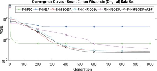
Figure 4. For the glass identification dataset, the algorithm’s convergence curves.

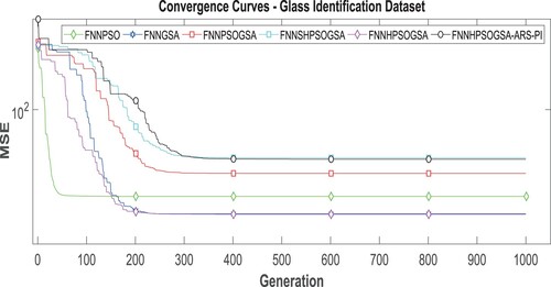
Figure 5. For LSD, the algorithm’s convergence curves.

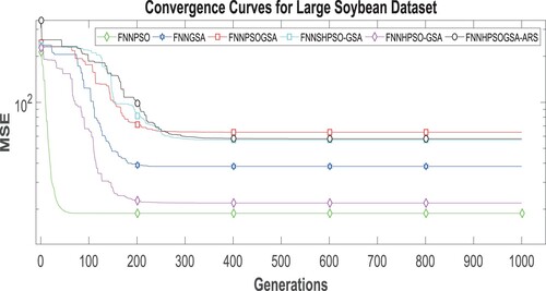
Table 2. WBCD dataset evaluation results.

Algorithm	MSE (AVE $\pm$ STD)	P-values	Classification rate %
FNNPSO	0.0226$\pm$0.0051	0.0891	97.6190
FNNGSA	0.0697$\pm$0.0568	0.0163	90.8425
FNNPSOGSA	0.0193$\pm$0.0071	0.2460	97.8022
FNNHPSOGSA	0.0468$\pm$0.0049	P < 0.0001	93.4066
FNNSHPSOGSA	0.0218 $\pm$ 0.0065	0.7081	98.1685
FNNHPSOGSA-ARS	0.0143$\pm$0.0046	0.8154	98.3516

Table 3. Iris dataset evaluation result.

Algorithm	MSE (AVE $\pm$ STD)	P-values	Classification rate %
FNNPSO	0.0769$\pm$0.0253	P < 0.0001	95.3333
FNNGSA	0.0825 $\pm$0.0267	P < 0.0001	96.6667
FNNPSOGSA	0.0329 $\pm$ 0.1014	0.9829	98.6667
FNNHPSOGSA	0.2629 $\pm$ 0.3026	0.9778	66.0000
FNNSHPSOGSA	0.0306$\pm$ 0.0745	0.7708	99.3365
FNNHPSOGSA-ARS	0.0223 $\pm$ 0.0073	0.9815	99.9667

Table 4. Car evaluation dataset evaluation result.

Algorithm	MSE (AVE $\pm$ STD)	P-values	Classification rate %
FNNPSO	0.1950 $\pm$ 0.3666	0.0089	94.6854
FNNGSA	0.0486 $\pm$ 0.0082	0.0089	93.9975
FNNPSOGSA	0.0224 $\pm$ 0.0099	0.4309	96.6667
FNNHPSOGSA	0.1379 $\pm$ 0.03950	0.0089	88.3463
FNNSHPSOGSA	0.0452 $\pm$ 0.0185	0.0942	97.1918
FNNHPSOGSA-ARS	0.0194 $\pm$ 0.0066	0.4792	97.6150

Table 5. Glass dataset evaluation result.

Algorithm	MSE (AVE $\pm$ STD)	P-values	Classification rate %
FNNPSO	0.1311 $\pm$ 0.1643	7.6546e-04	92.7305
FNNGSA	0. 1124 $\pm$ 0.0977	9.2532e-20	91.7511
FNNPSOGSA	0.1124 $\pm$ 0.0977	0.0486	94.0637
FNNHPSOGSA	0.0528 $\pm$ 0.3071	0.0091	89.6667
FNNSHPSOGSA	0.0432 $\pm$ 0.0590	0.0496	94.7863
FNNHPSOGSA-ARS	0.0064 $\pm$ 8.4760e-05	0.0431	95.3019

Table 6. Primary tumour dataset evaluation result.

Algorithm	MSE (AVE $\pm$ STD)	P-values	Classification rate %
FNNPSO	0.0955 $\pm$ 0.0709	0.0189	86.3337
FNNGSA	0.2918 $\pm$ 0.1411	5.6071e-12	87.4012
FNNPSOGSA	0.0247 $\pm$ 0.0239	0.0642	89.4940
FNNHPSOGSA	0.1548 $\pm$ 0.0711	0.0073	79.5333
FNNSHPSOGSA	0.0407 $\pm$ 0.0590	0.0781	90.3172
FNNHPSOGSA-ARS	0.0085 $\pm$ 0.0186	0.0396	91.1003

Table 7. LSD evaluation result.

Algorithm	MSE (AVE $\pm$ STD)	P-values	Classification rate %
FNNPSO	0.0235$\pm$0.0047	0.5481	79.7540
FNNGSA	0.0334$\pm$0.0039	0.0014	78.4515
FNNPSOGSA	0.0241$\pm$0.0029	0.4052	80.0434
FNNHPSOGSA	0.0332$\pm$0.0037	0.0015	73.7279
FNNSHPSOGSA	0.0174$\pm$0.0093	0.3348	84.3329
FNNHPSOGSA-ARS	0.0115$\pm$0.0092	0.6278	85.4776

There are three possible explanations for these results. Firstly, introducing the synchronous use of inertia weight and constriction factor ensured that particles in the swarm maintained a balanced exploration and exploitation throughout the search for the global optimum solution. Particles were restricted to search within the search boundary throughout the search, ensuring that the algorithm converged at the same locality. Closely following in order of increased robustness and stability are the PSOGSA and SHPSOGSA, which incorporate an effective balance between exploration and exploitation ability into PSO via GSA’s acceleration component. On binary datasets, we observe this improved outcome in Figure 3, where HPSOGSA-ARS, PSOGSA, and SHPSOGSA converge at 555th, 609th, and 804th iteration, respectively. The standard PSO shows the earliest convergence at the 110th iteration demonstrating its inherent weakness of premature convergence at a sub-optimal solution.

In contrast, HPSOGSA demonstrates the worst convergence ability by not converging even after 1000th iterations. This observation is mainly due to PSO’s ineffective hybridisation with GSA. HPSOGSA-ARS maintains the best convergence ability on multi-class datasets as it converges at the 515th iteration, whereas SHPSOGSA and PSOGSA show a competitive convergence strength at 454th and 420th iterations, respectively. HPSOGSA demonstrates a better convergence performance on multi-class datasets as shown by convergence at 358th and 306^th iterations on Figures 4 and 5, respectively.

Another possible explanation is that replacing PSO’s cognitive component with the acceleration component ensured that particles searched widely enough within the search boundary during the initial stages of the search process. Thus, enhanced diversity within the swarm accounted for the algorithm’s ability to find a solution near the global optima. This ability is evident in the best MSE values and the classification outcomes obtained by HPSOGSA-ARS and its closely related variants PSOGSA and SHPSOGSA, which possess a similar hybridisation technique. In these three closely related hybrid PSOGSA variants, the authors replaced the cognitive component of PSO with the acceleration component of GSA, leading to maximum exploration. Comparative to the hybrid strategy in these closely related variants, the implementation of the synchronous constriction factor and inertia weight accounted for the better performance of HPSOGSA-ARS over PSOGSA and SHPSOGSA in terms of classification accuracy and MSE values on both binary and multi-class datasets as recorded in Table 2–7.

Furthermore, our proposed algorithm overcomes the challenge of local optima entrapment, which has been proved by a better exploratory search outcome on binary and multi-class datasets in Figures 3 and 5 with convergence at 358th and 306th iterations, respectively. An explanation for this outcome is that, by incorporating an adaptive response strategy into PSO’s position update equation, a significant reduction in the number of stagnated particles in a sub-optimal solution occurred, which led to the conduction of further searches for the global optimum solution. The ARS is responsible for the high average classification values obtained by HPSOGSA-ARS across the selected benchmark datasets. Although PSOGSA and SHPSOGSA perform well by striving to maintain a balanced exploration and exploitation at different stages of the search for global optima, both algorithms do not have a mechanism that checks and enables stagnated particles to escape sub-optimal solution entrapment.

Although it is a widely held notion that hybridising PSO with other high-performing metaheuristics eventually results in an improved hybrid optimisation algorithm, our findings reveal that it is not always true. Whether the resulting hybrid algorithm will perform better than its constituent algorithms largely depend on how the algorithms were merged. As such, we offer a novel perspective that PSO’s position update equation can be modified to minimise the likelihood of early convergence leading to entrapment of particles in sub-optimal solution regions. Another well-held belief is that the introduction of inertia weight and constriction factor significantly enhances PSO’s search performance. Our method presents a new way of synchronising the inertia weight and constriction factor to ensure good exploration ability from the onset and a good exploitation ability during the final iteration stages.

Our study has two main limitations. Firstly, the computational cost of the proposed algorithm is relatively high. This observation is attributable to our proposed algorithm's numerous computational steps to achieve the desired outcome. Secondly, there isn’t much significant difference in the outcome of the proposed method compared to the peer algorithms used in this work, as revealed by the $p-values$ in Table 8. But in general, the results indicate a significant improvement compared to the standard PSO algorithm.

Table 8. Wilcoxon rank-sum test indicating P-values for binary and multi-class datasets.

Algorithm	Binary and Multi-class Datasets
	WBCD	Iris	Car Evaluation	Glass ID.	Primary Tumour	Large Soybean
	p-value	p-value	p-value	p-value	p-value	p-value
PSO	0.0891	P < 0.0001	0.0089	7.6546e-04	0.0189	0.5481
GSA	0.0163	P < 0.0001	0.0089	9.2532e-20	5.6071e-12	0.0014
PSOGSA	0.2460	0.9829	0.4309	0.0486	0.0642	0.4052
HPSOGSA	P < 0.0001	0.9778	0.0089	0.0091	0.0073	0.0015
SHPSOGSA	0.7081	0.7708	0.0942	0.0496	0.0781	0.3348
PSOGSA-ARS-PI	0.8154	0.9815	0.4792	0.0531	0.0596	0.6278

Bold indicates high significant values in terms of algorithms performances across the datasets.

4.4. Results of parametric studies

This section discusses the computational time, the key parameters, and their influence on the proposed FNN training algorithm’s performance. We begin by considering computational time analysis, changes in the number of particles, the number of iterations, the trap activation triggering value, and the number of neighbouring particles near the stagnated particle.

4.4.1. Computation time

This section presents a detailed analysis of the computational time our proposed HPSOGSA-ARS takes to complete execution on the six selected benchmark datasets compared to the closely related training algorithms implemented in this article. According to $t$-test, we perform 30 independent experimental runs on each algorithm and record all average CPU times of each FNN training method. The experiment is conducted using MATLAB R2018a programming environment with a CPU specification of Intel(R) Core (T.M.) i7-4800MQ CPU @ 2.70 GHz (8 CPUs), ∼2.7 GHz, 8GB RAM.

Table 10 presents the observed computational time for training an FNN and classifying a test sample on the selected datasets with the best average time emphasised. It is observed in Table 10 that, except for HPSOGSA, the proposed HPSOGSA-ARS algorithm is diminutively more time-consuming than the remaining variants on all the datasets. This observed increase in the computational time of HPSOGSA-ARS is due to its synchronous execution of the constriction factor and inertia weight in addition to the incorporation of the Adaptive Response Strategy. Although undesirable, the time spent to execute HPSOGSA-ARS is worthwhile since the performance of PSO is ultimately improved.

Table 9. Comparing the number of iterations until convergence for binary and multiclass datasets.

Proposed FNN Training Method	Number of iterations on Binary Class dataset	Number of iterations on Multi-class datasets
HPSOGSA-ARS	400–600 iterations	400–500 iterations
EXISTING
FNNPSO	100 iterations	Less than 100 iterations
FNNGSA	300 iterations	200–300 iterations
FNNPSOGSA	800 iterations	300–400 iterations
FNNSHPSOGSA	1000 iterations	400 iterations
FNNHPSOGSA	More than 1000 iterations	200–250 iterations

Table 10. Average computation time (seconds) of the algorithms on a selected binary and multiclass benchmark datasets.

Benchmark Dataset	WBCD	Iris	Car Evaluation	Glass ID.	Primary Tumour	Large Soybean
PSO	1.04e$+$00	3.29e$+$00	4.58e$+$00	5.83e$+$00	5.10e$+$00	7.94e$+$00
GSA	5.82e$+$00	6.40e$+$00	7.89e$+$00	1.05e$+$01	3.75e$+$01	1.30e$+$01
PSOGSA	7.73e$+$00	9.34e$+$00	2.25e$+$01	2.62e$+$01	5.14e$+$01	8.14e$+$01
HPSOGSA	2.09e$+$03	2.96e$+$03	3.44e$+$03	1.07e$+$01	8.54e$+$04	1.38e$+$01
SHPSOGSA	4.77e$+$01	2.77e$+$01	3.78e$+$01	4.51e$+$01	6.09e$+$02	3.44e$+$02
HPSOGSA-ARS	6.62e$+$02	5.99e$+$01	5.24e$+$02	4.69e$+$01	6.40e$+$02	3.56e$+$02

4.4.2. Effect of changes in number of particles and maximum iterations on the performance of HPSOGSA-ARS

This section discusses the effects of altering parameters, namely: number of particles and iterations, on the performance of HPSOGSA-ARS. We conducted this parametric investigation by alternating the number of particles from 20 to 40 in steps of 10 particles while alternating the maximum iterations from 500 to 1500 in steps of 500 iterations on the benchmark datasets. Figures 6 and 8 are visual representations of the parametric study outcome of HPSOGSA-ARS with its comparing variants when the maximum iteration is fixed at 500 and the number of particles being gradually increased from 20 to 40 in steps of 10 particles. Contrastingly, Figures 7 and 9 depict the parametric study outcome when the number of particles is fixed at 30, and the number of iterations gradually increases in steps of 500. It was observed from the experiment that when the maximum iteration is set at 500, increasing the number of particles generally increases accuracy on all the benchmark datasets. Moreover, we recorded the highest accuracy when the maximum iteration was fixed at 1500 and the number of particles at 30.

Figure 6. Based on various no. of particles considering the classification accuracy (WBCD).

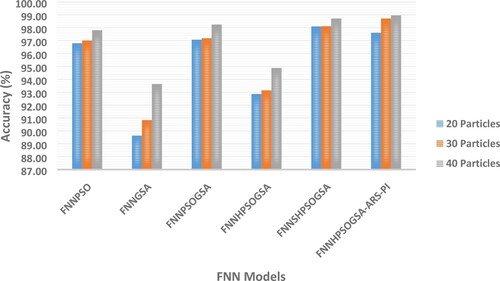
Figure 7. Based on various max iterations considering the classification accuracy (WBCD).

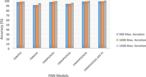
Figure 8. Based on no. of particles considering the classification accuracy (LSD).

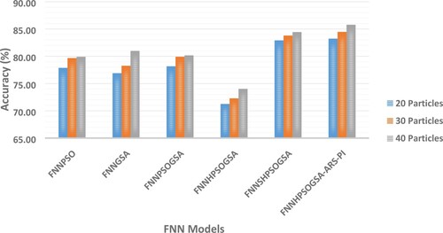
Figure 9. Based on various max iterations considering the classification accuracy (LSD).

HPSOGSA-ARS obtained an increased accuracy value according to Figures 6, 8, as well as Tables 11 and 12. The possible reason for this outcome is that keeping the maximum number of iterations at 500 while increasing the number of particles from 20 to 40 means more particles will extensively search within the search space. Consequently, the global optimum solution is easily located within a relatively shorter time with little effort. Similarly, HPSOGSA-ARS obtained an increased accuracy value according to Figures 7 and 9. The possible reason for this outcome is that keeping the number of particles at 30 while increasing the number of iterations from 500 to 1500 in steps of 500 means few particles will extensively search within the search space for an extended period. Additionally, the improved strategies ensure that particles explore widely within the search space while avoiding sub-optimal solution entrapment.

Table 11. Classification accuracy of FNN models on wisconsin breast cancer dataset.

No. of Particles	20			30
Max iteration	500	30	40	500	1000	1500
FNNPSO	96.80%	97.01%	97.82%	97.01%	97.62%	98.44%
FNNGSA	89.63%	90.84%	93.63%	90.84%	90.84%	94.67%
FNNPSOGSA	97.08%	97.17%	98.25%	97.17%	97.80%	99.27%
FNNHPSOGSA	92.87%	93.15%	94.87%	93.15%	93.41%	95.33%
FNNSHPSOGSA	98.09%	98.12%	98.72%	98.12%	98.17%	99.45%
FNNHPSOGSA-ARS	97.62%	98.72%	98.95%	98.72%	98.35%	99.95%

Table 12. Classification accuracy of FNN models on LSD.

No. of particles	20			30
Max iteration	500	30	40	500	1000	1500
FNNPSO	77.87%	79.68%	79.89%	79.68%	79.75%	80.28%
FNNGSA	76.89%	78.24%	80.95%	78.24%	78.45%	79.89%
FNNPSOGSA	78.17%	79.91%	80.13%	79.91%	80.04%	80.26%
FNNHPSOGSA	71.23%	72.31%	74.02%	72.31%	73.73%	75.67%
FNNSHPSOGSA	82.90%	83.82%	84.44%	83.82%	84.33%	86.04%
FNNHPSOGSA-ARS	83.25%	84.48%	85.75%	84.48%	85.48%	87.72%

As such, regarding HPSOGSA-ARS as a stochastic search algorithm, an increased number of iterations only increases the likelihood of global optimum solution attainment irrespective of its starting number of particles.

4.4.3. Effect of the number of nearest neighboring particles on HPSOGSA-ARS’ performance

This section performs experiments to determine the optimal number of particles near a stagnated particle upon which a stagnated particle depends to adjust its position. We do this by altering the number of closest particles and exploring their effects on the performance of HPSOGSA-ARS. According to the result of our experiment, we concluded that the optimal number of nearest particles is 7. This conclusion was based on the observation that when the maximum iteration was set at 1000, the best MSE and the highest classification accuracy were obtained when the nearest particles were seven.

It can be observed in Table 13 that the average MSE values and classification accuracy values increased as the nearest number of particles increased from 2-6, peaked at 7, and then steadily declined from 8 upwards. As such, we cannot conclude that an increased number of nearest particles leads to a better performance of the algorithm. However, since the algorithm is stochastic, the reason for 7 being the optimal value is intrinsic, which could not be pointed out precisely but rather accurately determined via experimentation.

Table 13. Number of nearest neighbouring particles parameter sensitivity on datasets.

	Datasets
	Binary (WBCD)		Multi-class (LSD)
Number Neighbouring particles	Average MSE	Accuracy rate (%)	Average MSE	Accuracy rate (%)
2	0.1523	94.9138	0.0774	78.9942
3	0.0974	95.6667	0.0691	79.2259
4	0.0322	96.8371	0.0370	82.9674
5	0.0248	97.0248	0.0174	85.0931
6	0.0188	98.0012	0.0201	83.8750
7	0.0143	98.3516	0.0115	85.4776
8	0.0401	93.9005	0.0184	84.6021
9	0.0748	92.0136	0.0289	83.2337
10	0.2109	91.8941	0.0231	83.8867

4.4.4. Effect of the trap activation triggering value on HPSOGSA-ARS’ performance

The Trap Activation value used to trigger the Adaptive Response Strategy (ARS) is an influential parameter that, when altered, will significantly affect the FNN optimisation outcome. In this section, we seek to determine the optimal trap activation value. We do this by adjusting the value of the trap activation parameter and exploring its effect on the performance of the HPSOGSA-ARS algorithm. Our experiment found the optimal trap activation value to be 3. This observed result stems from the fact that by keeping the trap activation value at three (3) while maintaining the maximum iteration and the number of particles at 1000 and 30, respectively, we obtain the best MSE and highest classification accuracy values.

The results presented in Table 14 indicate that HPSOGSA-ARS is a stable and robust algorithm on binary datasets. The stability and robustness outcome of HPSOGSA-ARS has been derived from the observation that the HPSOGSA-ARS algorithm attains the best convergent ability with an adequately balanced exploration and exploitation capacity in addition to best MSE and standard deviation values. Contrary to the previous observation in Table 14, we observed that although the HPSOGSA-ARS algorithm exhibited a slightly early convergence on multi-class datasets, it attained the best performance in terms of MSE and standard deviation values.

Table 14. Trap activation value parameter sensitivity on datasets.

	Datasets
	Binary (WBCD)		Multi-class (Glass ID)
Trap Activation values	MSE (AVE $\pm$ STD)	Iterations	MSE (AVE $\pm$ STD)	Iterations until convergence
1	0.0164$\pm$0.0050	520	0.1114 $\pm$ 0.0961	265
2	0.0152$\pm$0.0048	570	0.0853$\pm$0.0742	380
3	0.0143$\pm$0.0046	600	0.0064 $\pm$ 8.4760e-05	400
4	0.0268$\pm$0.0066	711	0.0071$\pm$7.7039e-04	440
5	0.0391$\pm$0.0074	845	0.0169$\pm$ 9.3760e-03	670
6	0.0527$\pm$0.0091	967	0.0208$\pm$ 9.9938e-02	895

As stochastic algorithms are dynamic, it is challenging to explain precisely their intrinsic behaviour from a theoretical perspective. We, therefore, resort to explaining the possible reason for this outcome experimentally. When the trap activation value is less, the algorithm triggers the Adaptive Response Strategy (ARS) early enough to cause a stagnated particle to jump out of stagnation early. ARS action gives such particles ample time to explore and locate the global optimum solution at fewer iterations. On the other hand, a higher trap activation value implies a comparatively long time for the ARS to be triggered to enable stagnated particles to jump out of sub-optimal solutions. Thus, a higher trap activation leads to more time to search and locate the global optimum solution with more iterations.

4.4.5. Effectiveness of constriction factor and adaptive response strategies

This section performs experiments to determine the efficacy of constrictor factor and adaptive response strategies by comparing the convergence outcomes of HPSOGSA-ARS and HPSOGSA. The algorithm with constriction and adaptive response strategies is denoted HPSOGSA-ARS, else HPSOGSA. The experiment is performed on the six benchmark datasets described in Table 1, and the parameter configurations are set per Section 4, subsection one. Figure 10 depicts the outcome of the experiment.

Figure 10. Convergence curves of HPSOGSA and HPSOGSA-ARS on datasets.

The test results on all datasets depict that HPSOGSA-ARS have a better average diversity than HPSOGSA. Across all the implemented datasets, we observe that the average diversity of particles in HPSOGSA-ARS from the early stages of iteration to the latter stages is better when compared to that of HPSOGSA. Specifically, HPSOGSA achieves a better average diversity in the early stages symbolising a good exploration ability. In contrast, it is observed that during the later stages of the search, the HPSOGSA algorithm is unable to appropriately transition search from exploration into exploitation leading to stagnation of particles as indicated by the straight line. On the WBCD in Figure 10(a), Iris dataset in Figure 10(b), Car Eval dataset in Figure 10(c), Glass ID dataset in Figure 10(d), Large Soybean dataset in Figure 10(e) and on Primary Tumour dataset on Figure 10(f), we observe this line from the 3000th, 2000th, 3200th, 5700th, 6100th and 4900th iterations and beyond respectively.

On the other hand, we observe that the HPSOGSA-ARS search process similarly obtains a good exploration during the early phase of the search and can transition from exploration into exploitation with increased iteration. Additionally, we observe in the search process of the HPSOGSA-ARS that anytime stagnation occurs (indicated by the intermittent straight lines), the adaptive response strategy is activated to unfold particles leading to a continued search until the attainment of a global optimum. This group of tests validates the contributions of the constriction factor and the adaptive response strategy to prevent premature convergence and ensure balanced exploratory and exploitation searches.

5. Conclusions

This article researched the previous implementation of the Particle swarm optimisation (PSO) algorithm in optimising Feedforward Neural Networks (FNN) and improved upon those works by incorporating novel strategies. The improvement strategy hybridises PSO with the Gravitational search algorithm (GSA) and includes an adaptive response strategy and a constriction factor (HPSOGSA-ARS). HPSOGSA-ARS was then used to optimise an FNN to perform classification. When evaluated on six selected diversified benchmark datasets, FNN-HPSOGSA-ARS demonstrated a better performance in avoiding sub-optimal solutions entrapment and achieving a better convergence rate. Our findings confirm that when we hybridise PSO with another heuristic algorithm good at exploration, it complements PSO’s weakness of early convergence. Additionally, our results demonstrated that increased performance is achieved when a sub-optimal solution stagnation escape mechanism is incorporated into the PSO algorithm.

Moreover, our study offers a novel perspective on position update equation improvement, modifying PSO’s inertia weight and constriction factor so that they work jointly in a manner that leads to PSO’s improved performance. It is noteworthy that we can use other metaheuristics in place of PSO or GSA to optimise FNNs. Examples of these metaheuristics are monarch butterfly optimisation (MBO)(Xie & Wang, 2021), earthworm optimisation algorithm (EWA)(Prasad et al., 2021), elephant herding optimisation (EHO)(Kilany et al., 2021), moth search (M.S.) algorithm(Feng & Wang, 2021), Slime mould algorithm (SMA)(Precup et al., 2021), and Harris hawks optimisation (HHO)(Mary et al., 2021) algorithm. However, we can only obtain an optimal performance when we resolve their limitations effectively, as this work does.

Future work can focus on any of these directions as follows: firstly, by extending HPSOGSA-ARS to handle multi-objective optimisation problems, complex classification problems, and gene selection for cancer classification. Secondly, by modifying the position update equation to enhance the tendency of PSO to avoid sub-optimal solution entrapment, thirdly, furthering the improvement approaches of PSO that has to do with implementing inertia weight and constriction factor simultaneously to obtain a balanced exploration and exploitation. fourthly, hybridising other metaheuristics that possesses an excellent exploratory search ability with PSO with or without different improvement strategies to solve multi-objective optimisation real-world challenges. Finally, applying the resulting algorithm to solve optimisation tasks in other fields of life such as Agriculture, Engineering, Business, etc.

Acknowledgments

The authors express their gratitude to all unnamed reviewers for their inputs.

Disclosure statement

No potential conflict of interest was reported by the author(s).

Additional information

Funding

Publication expenses are sponsored by the National Natural Science Foundation of China [Nos. 61976108 and 61572241].

References

- Amponsah, A. A., Han, F., Osei-Kwakye, J., Bonah, E., & Ling, Q.H. (2021). An improved multi-leader comprehensive learning particle swarm optimisation based on gravitational search algorithm. Connection Science, 33(4), 803–834. https://doi.org/10.1080/09540091.2021.1900072
- Andrew, F., & Asuncion, A. (2011). UCI Machine Learning Repository, 2010, 15, 22. http://archive.ics.uci.edu/ml
- Bohat, V. K., & Arya, K. (2018). An effective gbest-guided gravitational search algorithm for real-parameter optimization and its application in training of feedforward neural networks. Knowledge-Based Systems, 143, 192–207. https://doi.org/10.1016/j.knosys.2017.12.017
- Christo, V. E., Nehemiah, H. K., Nahato, K. B., Brighty, J., & Kannan, A. (2020). Computer assisted medical decision-making system using genetic algorithm and extreme learning machine for diagnosing allergic rhinitis. International Journal of Bio-Inspired Computation, 16(3), 148–157. https://doi.org/10.1504/IJBIC.2020.111279
- Cui, Z., Xue, F., Cai, X., Cao, Y., Wang, G.G., & Chen, J. (2018). Detection of malicious code variants based on deep learning. IEEE Transactions on Industrial Informatics, 14(7), 3187–3196. https://doi.org/10.1109/TII.2018.2822680
- dos Santos Coelho, L. (2008). A quantum particle swarm optimizer with chaotic mutation operator. Chaos, Solitons & Fractals, 37(5), 1409–1418. https://doi.org/10.1016/j.chaos.2006.10.028
- Eftimov, T., Korošec, P., & Seljak, B. K. (2017). A novel approach to statistical comparison of meta-heuristic stochastic optimization algorithms using deep statistics. Information Sciences, 417, 186–215. https://doi.org/10.1016/j.ins.2017.07.015
- Eyoh, I. J., Umoh, U. A., Inyang, U. G., & Eyoh, J. E. (2020). Derivative-based learning of interval type-2 intuitionistic fuzzy logic systems for noisy regression problems. International Journal of Fuzzy Systems, 22(3), 1007–1019. https://doi.org/10.1007/s40815-020-00806-z
- Falahiazar, L., & Shah-Hosseini, H. (2018). Optimisation of engineering system using a novel search algorithm: The spacing multi-objective Genetic algorithm. Connection Science, 30(3), 326–342. https://doi.org/10.1080/09540091.2018.1443319
- Feng, Y., & Wang, G.G. (2021). A binary moth search algorithm based on self-learning for multidimensional knapsack problems. Future Generation Computer Systems, 126, 48–64. https://doi.org/10.1016/j.future.2021.07.033
- Han, F., Jiang, J., Ling, Q. H., & Su, B. Y. (2019). A survey on metaheuristic optimization for random single-hidden layer feedforward neural network. Neurocomputing, 335, 261–273. https://doi.org/10.1016/j.neucom.2018.07.080
- Huang, C. P., Xiong, W. L., & Xu, B. G. (2008). Influnce of inertia weight on astringency of particle swarm algorithm and its improvement. Computer Engineering, 34(12), 31–33. https://doi.org/10.1080/10286600801908949
- Huang, H.S., Fan, Q.S., Wei, J.N., & Huang, D. (2019). An intelligent fault identification method of rolling bearings based on SVM optimized by improved GWO. Systems Science Control Engineering, 7(1), 289–303. https://doi.org/10.1080/21642583.2019.1650673
- Jiang, J., Hu, G., Li, X., Xu, X., Zheng, P., & Stringer, J. (2019). Analysis and prediction of printable bridge length in fused deposition modelling based on back propagation neural network. Virtual Physical Prototyping, 14(3), 253–266. https://doi.org/10.1080/17452759.2019.1576010
- Jiang, S., Ji, Z., & Shen, Y. (2019). A novel hybrid particle swarm optimization and gravitational search algorithm for solving economic emission load dispatch problems with various practical constraints. International Journal of Electrical Power, 55, 628–644. https://doi.org/10.1016/j.ijepes.2013.10.006
- Karamichailidou, D., Kaloutsa, V., & Alexandridis, A. (2021). Wind turbine power curve modeling using radial basis function neural networks and tabu search. Renewable Energy, 163, 2137–2152. https://doi.org/10.1016/j.renene.2020.10.020
- Kilany, M., Zhang, C., & Li, W. (2021). Optimization of urban land cover classification using an improved elephant herding optimization algorithm and random forest classifier. International Journal of Remote Sensing, 42(15), 5731–5753. https://doi.org/10.1080/01431161.2021.1931533
- Konda, S. R., Panwar, L. K., Panigrahi, B. K., Kumar, R., & Gupta, V. (2021). Binary fireworks algorithm application for optimal schedule of electric vehicle reserve in traditional and restructured electricity markets. International Journal of Bio-Inspired Computation, 18(1), 38–48. https://doi.org/10.1504/IJBIC.2021.117430
- Lalwani, S. (2021). Design and implementation of bi-level artificial bee colony algorithm to train hidden markov models for performing multiple sequence alignment of proteins. International Journal of Swarm Intelligence, 6(1), 48–64. https://doi.org/10.1504/IJSI.2021.114765
- Lei, Z., Gao, S., Gupta, S., Cheng, J., & Yang, G. (2020). An aggregative learning gravitational search algorithm with self-adaptive gravitational constants. Expert Systems with Applications, 152, 113396, https://doi.org/10.1016/j.eswa.2020.113396.
- Lin, J., & Yu, J. (2011, 27th–29th May). Weighted naive Bayes classification algorithm based on particle swarm optimization. 2011 IEEE 3rd International Conference on Communication software and networks.
- Liu, A., Li, P., Deng, X., & Ren, L. (2021). A sigmoid attractiveness based improved firefly algorithm and its applications in IIR filter design. Connection Science, 33(1), 1–25. https://doi.org/10.1080/09540091.2020.1742660
- Liu, H.B., Wang, X.K., & Tan, G.Z. (2006). Convergence analysis of particle swarm optimization and its improved algorithm based on chaos. Control and Decision, 21(6), 636.
- Malela-Majika, J.-C. (2021). New distribution-free memory-type control charts based on the Wilcoxon rank-sum statistic. Quality Technology & Quantitative Management, 18(2), 135–155. https://doi.org/10.1080/16843703.2020.1753295
- Mary, A. H., Miry, A. H., & Miry, M. H. (2021). An optimal robust state feedback controller for the AVR system-based Harris hawks optimization algorithm. Electric Power Components and Systems, 48(16-17), 1684–1694.
- Mirjalili, S., Hashim, S. Z. M., & Sardroudi, H. M. (2012). Training feedforward neural networks using hybrid particle swarm optimization and gravitational search algorithm. Applied Mathematics Computation, 218(22), 11125–11137. https://doi.org/10.1016/j.amc.2012.04.069
- Mirjalili, S., Hashim, S. Z. M., & Sardroudi, H. M. J. A. M. Computation. (2012). Training feedforward neural networks using hybrid particle swarm optimization and gravitational search algorithm. Applied Mathematics and Computation, 218(22), 11125–11137. https://doi.org/10.1016/j.amc.2012.04.069
- Mukherjee, R. P., Roy, P. K., & Pradhan, D. K. (2021). An Efficient FNN model with chaotic oppositional based SCA to solve classification problem. IETE Journal of Research, 1–19. https://doi.org/10.1080/03772063.2021.1948923
- Nagra, A. A., Han, F., Ling, Q. H., Abubaker, M., Ahmad, F., Mehta, S., & Apasiba, A. T. (2019). Hybrid self-inertia weight adaptive particle swarm optimisation with local search using C4. 5 decision tree classifier for feature selection problems. Connection Science, 32(1), 16–36. https://doi.org/10.1080/09540091.2019.1609419
- Nayak, S. K., Rout, P. K., Jagadev, A. K., & Swarnkar, T. (2018). Elitism-based multi-objective differential evolution with extreme learning machine for feature selection: A novel searching technique. Connection Science, 30(4), 362–387. https://doi.org/10.1080/09540091.2018.1487384
- Neshat, M., Pourahmad, A. A., & Rohani, Z. (2020). Improving the cooperation of fuzzy simplified memory A* search and particle swarm optimisation for path planning. International Journal of Swarm Intelligence, 5(1), 1–21. https://doi.org/10.1504/IJSI.2020.106388
- Prasad, D. S., Chanamallu, S. R., & Prasad, K. S. (2021). Mitigation of ocular artifacts for EEG signal using improved earth worm optimization-based neural network and lifting wavelet transform. Computer Methods in Biomechanics and Biomedical Engineering, 24(5), 551–578. https://doi.org/10.1080/10255842.2020.1839893
- Precup, R.E., David, R.C., Roman, R.C., Szedlak-Stinean, A.-I., & Petriu, E. M. (2021). Optimal tuning of interval type-2 fuzzy controllers for nonlinear servo systems using Slime mould algorithm. International Journal of Systems Science. https://doi.org/10.1080/00207721.2021.1927236
- Radosavljević, J., Klimenta, D., Jevtić, M., & Arsić, N. (2018). Optimal Power flow using a Hybrid Optimization algorithm of particle swarm optimization and gravitational search algorithm. Electric Power Components and Systems, 43(17), 1958–1970. https://doi.org/10.1080/15325008.2015.1061620
- Ram, B. D., & Rao, B. S. (2018). An Efficient ids based on fuzzy firefly optimization and fast learning network. International Journal of Engineering & Technology, 7(4.36), 557–561. https://doi.org/10.14419/ijet.v7i4.36.24137
- Rashedi, E., Nezamabadi-Pour, H., & Saryazdi, S. (2009). GSA: A gravitational search algorithm. Information Sciences, 179(13), 2232–2248. https://doi.org/10.1016/j.ins.2009.03.004
- Rashedi, E., Nezamabadi-Pour, H., & Saryazdi, S. (2010). BGSA: Binary gravitational search algorithm. Natural Computing, 9(3), 727–745. https://doi.org/10.1007/s11047-009-9175-3
- Rather, S. A., Bala, P. S., Ashokan, P. L., & Mercangöz, B. A. (2021). Training multi-layer perceptron using hybridization of chaotic gravitational search algorithm and particle swarm optimization. In Applying particle swarm optimization (pp. 233–262). Springer.
- Russell, E., & James, K. (1995, 4th–6th October). A new optimizer using particle swarm theory. MHS'95. Proceedings of the sixth International symposium on micro Machine and human science.
- Sağ, T., & Jalil, Z. A. J. (2021). Vortex search optimization algorithm for training of feed-forward neural network. International Journal of Machine Learning and Cybernetics, 12(5), 1517–1544. https://doi.org/10.1007/s13042-020-01252-x
- Saremi, S., Mirjalili, S., & Andrew, L. (2014). Biogeography-based optimization with chaos. Neural Computing Applications, 25(5), 1077–1097. https://doi.org/10.1007/s00521-014-1597-x
- Šešum-Čavić, V. (2020). A survey of swarm-inspired metaheuristics in P2P systems: Some theoretical considerations and hybrid forms. International Journal of Swarm Intelligence, 5(2), 244–282. https://doi.org/10.1504/IJSI.2020.111173
- Singh, J., Banka, H., & Verma, A. K. (2018, 15th–17th March). Analysis of slope stability and detection of critical failure surface using gravitational search algorithm. 2018 4th International Conference on recent Advances in information Technology (RAIT).
- Sreeja, N. K. (2019). A weighted pattern matching approach for classification of imbalanced data with a fireworks-based algorithm for feature selection. Connection Science, 31(2), 143–168. https://doi.org/10.1080/09540091.2018.1512558
- Suganthan, P. N. (2018). On non-iterative learning algorithms with closed-form solution. Applied Soft Computing, 70, 1078–1082. https://doi.org/10.1016/j.asoc.2018.07.013
- Sugiyama, T., Kutsuzawa, K., Owaki, D., & Hayashibe, M. (2021). Individual deformability compensation of soft hydraulic actuators through iterative learning-based neural network. Bioinspiration & Biomimetics, 16(5), 056016. https://doi.org/10.1088/1748-3190/ac1b6f.
- Wang, G., Guo, L., & Duan, H. (2013). Wavelet neural network using multiple wavelet functions in target threat assessment. The Scientific World Journal, 2013, 632437. https://doi.org/10.1155/2013/632437
- Wang, G. G., Lu, M., Dong, Y. Q., & Zhao, X. J. (2016). Self-adaptive extreme learning machine. Neural Computing and Applications, 27(2), 291–303. https://doi.org/10.1007/s00521-015-1874-3
- Wei, J.Y., Sun, Y.H. & Su, X.N. (2010). A document clustering algorithm using particle swarm optimization. J. Chin. Soc. Sci. Tech. Inf, 29(3), 428–432.
- Wilcoxon, F., Katti, S. K., & Wilcox, R. A. (1970). Critical values and probability levels for the Wilcoxon rank sum test and the Wilcoxon signed rank test. Selected Tables in Mathematical Statistics, 1, 171–259.
- Hu, X.H., & Eberhart, R. (2002, 12th–17th May). Multiobjective optimization using dynamic neighborhood particle swarm optimization. In Proceedings of the 2002 congress on evolutionary computation. CEC'02 (Cat. No. 02TH8600).
- Xie, L., & Wang, G.-G. (2021). Monarch butterfly optimization (handbook of AI-based metaheuristics (pp. 361-392. CRC Press.
- Yang, J., & Ma, J. (2019). Feed-forward neural network training using sparse representation. Expert Systems with Applications, 116, 255–264. https://doi.org/10.1016/j.eswa.2018.08.038
- Yang, X. S. (2010). A new metaheuristic bat-inspired algorithm (nature inspired cooperative strategies for optimization (NICSO 2010) (pp. 65-74). Springer.
- Yi, J.H., Wang, J., & Wang, G.-G. (2016). Improved probabilistic neural networks with self-adaptive strategies for transformer fault diagnosis problem. Advances in Mechanical Engineering, 8(1). https://doi.org/10.1177/1687814015624832
- Shi, Y.H., & Eberhart, R. (1998, 4th–9th May). A modified particle swarm optimizer. 1998 IEEE international conference on evolutionary computation proceedings. IEEE world congress on computational intelligence.
- Zemmal, N., Azizi, N., Sellami, M., Cheriguene, S., & Ziani, A. (2021). A new hybrid system combining active learning and particle swarm optimisation for medical data classification. International Journal of Bio-Inspired Computation, 18(1), 59–68. https://doi.org/10.1504/IJBIC.2021.117427
- Zhang, J., Li, Y., Xiao, W., & Zhang, Z. (2020). Non-iterative and fast deep learning: Multilayer extreme learning machines. Journal of the Franklin Institute, 357(13), 8925–8955. https://doi.org/10.1016/j.jfranklin.2020.04.033
- Zhang, J. R., Zhang, J., Lok, T. M., & Lyu, M. R. (2007). A hybrid particle swarm optimization–back-propagation algorithm for feedforward neural network training. Applied Mathematics and Computation, 2(185), 1026–1037. https://doi.org/10.1016/j.amc.2006.07.025
- Zhang, Z., Zhang, A., Sun, C., Xiang, S., Guan, J., & Huang, X. (2021). Research on air traffic flow forecast based on ELM non-iterative algorithm. Mobile Networks and Applications, 26(1), 425–439. https://doi.org/10.1007/s11036-020-01679-0