An improved Monte Carlo Tree Search approach to workflow scheduling

Abstract

Workflow computing has become an essential part of many scientific and engineering fields, while workflow scheduling has long been a well-known NP-complete research problem. Major previous works can be classified into two categories: heuristic-based and guided random-search-based workflow scheduling methods. Monte Carlo Tree Search (MCTS) is a recently proposed search methodology with great success in AI research on game playing, such as Computer Go. However, researchers found that MCTS also has potential application in many other domains, including combinatorial optimization, task scheduling, planning, and so on. In this paper, we present a new workflow scheduling approach based on MCTS, which is still a rarely explored direction. Several new mechanisms are developed for the major steps in MCTS to improve workflow execution schedules further. Experimental results show that our approach outperforms previous methods significantly in terms of execution makespan.

KEYWORDS:

• Monte Carlo Tree Search
• workflow scheduling
• parallel processing

I. Introduction

As the computational structure of modern scientific and engineering applications grows ever more complex and large-scale, workflow computing has become an inevitable parallel processing model. To improve computational performance, workflow scheduling (Topcuoglu et al., 2002) has become an important research topic on modern parallel processing platforms, including various high-performance computing platforms and cloud computing environments. There are a lot of methods proposed to resolve the challenging NP-complete workflow scheduling problem in the literature. Most of them are heuristic-based algorithms like HEFT (Topcuoglu et al., 2002), PEFT (Arabnejad & Barbosa, 2014), and IPPTS (Djigal et al., 2021). Another well-known category of workflow scheduling approaches is based on meta-heuristic methods (Keshanchi et al., 2017; Xu et al., 2014), e.g. genetic algorithm (Srinivas & Patnaik, 1994) and other evolutionary algorithms.

Search based approaches were less considered in the previous workflow scheduling studies because of the search space explosion problem, especially when dealing with large scale workflows and parallel computing platforms. However, the recent development of advanced search methods has made search-based approaches a potentially promising direction for workflow scheduling. Monte Carlo Tree Search (MCTS) (Browne et al., 2012) is one of the most well-known advanced search methods, which has shown great performance in several applications domains (Chaslot et al., 2006).

Traditionally, MCTS was usually used in computer programs playing turn-based-strategy games, such as Go, chess, shogi, and poker. However, some previous research works have tried to apply it to solve specific optimization problems, such as production management (Chaslot et al., 2006), and found that it has the potential to outperform commonly used heuristic-based algorithms. Recently, MCTS was applied to solve the workflow scheduling problem in (Liu et al., 2019). In addition to applying the traditional MCTS method, they also developed a pruning algorithm to reduce the search space in MCTS for improving search efficiency and effectiveness. The proposed approach leverages the idea of branch-and-bound and is called MCTS-BB (Liu et al., 2019).

The experimental results in (Liu et al., 2019) show that MCTS outperforms well-known heuristic algorithms for workflow scheduling, including HEFT, PEFT and CPOP (Topcuoglu et al., 2002). However, the experimental results also reveal that in general, the performance of MCTS-BB is worse than the original MCTS approach, indicating that the proposed pruning algorithm is not as effective as expected. The pruning algorithm in (Liu et al., 2019) relies on the makespan of the current partial schedule and the length of the critical path among unscheduled tasks to determine the upper bound guiding the search process. In this paper, we present new pruning and heuristic-guiding mechanisms to further improve the performance of MCTS in workflow scheduling. Experimental results show that our new approaches can achieve better performance than the original MCTS and MCTS-BB methods proposed in (Liu et al., 2019).

The remainder of this paper is organized as follows. In the next section, we present the formulation of the workflow scheduling problem. Section III discusses related works of heuristic-based and guided random-search-based workflow scheduling methods. Section IV illustrates how MCTS could be applied to solve the workflow scheduling problem and presents the MCTS-BB methods in (Liu et al., 2019). Section V describes our new heuristic guided MCTS approach for workflow scheduling. Section VI presents the overall performance evaluation of our improved MCTS approach for workflow scheduling with a comparison to well-known previous methods in the literature. Section VII concludes this paper and sheds some light on promising future research directions.

II. Workflow scheduling problem

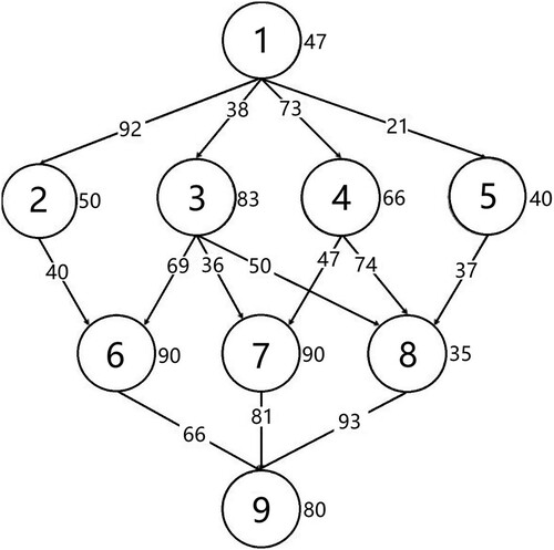
In most workflow scheduling research works (Arabnejad & Barbosa, 2014; Liu et al., 2019; Topcuoglu et al., 2002), a workflow is usually represented by a Directed Acyclic Graph (DAG), i.e. $G=(V,E)$, for describing the inter-task structure, where V represents the set of nodes and $E$ is the set of edges. Figure 1 shows a workflow example represented by a DAG. Each node in the workflow represents a computational task with the annotated value indicating the required execution time. The directed edges between tasks represent the computational or data interdependence among them and thus reduce potential task parallelism and enforce specific execution order of all tasks. The number next to an edge indicates the required data transfer time between tasks. The workflow scheduling problem on a parallel computing platform is to determine the start time and allocated processor for each task in a workflow, aiming for optimizing a specific goal, e.g. execution makespan.

Figure 1. Workflow structure represented by a DAG.

When speed heterogeneity of processors is considered in workflow scheduling, the required execution time for each task in the DAG is usually assigned to the average value of execution time across all processors in the system (Arabnejad & Barbosa, 2014; Topcuoglu et al., 2002) as follows, where $w_{i,j}$ is the required execution time for task $i$ on processor $j$ and there are total $q$ processors in the system. (1) $\begin{array}{r}\overline{w_i}=\sum _{j=1}^q\frac{w_{i,j}}{q}\end{array}$(1) For two tasks $i,j$ executed on processor $m,n$ respectively, the required communication time $c_{i,j}$ for the edge connecting nodes $n_i$ and $n_j$ in the DAG is usually measured by summing up the latency $L_{m,n}$ and the data transfer time which could be calculated by dividing the data size $\text{dat}{\text{a}}_{i,j}$ by the data transfer rates $B_{m,n}$, i.e. network bandwidth, between the two processors running tasks i and j. (2) $\begin{array}{r}{c}_{i,j}=L_{m,n}+\frac{\text{dat}{\text{a}}_{i,j}}{B_{m,n}}\end{array}$(2)

When a heterogeneous computing environment is concerned, the weight on an edge $c_{i,j}$ in the workflow’s DAG could be represented by the average communication time of transfer the data of size $\text{dat}{\text{a}}_{i,j}$ across all possible network links in the system as follows. (3) $\begin{array}{r}\overline{c_{i,j}}=\overline{L}+\frac{\text{dat}{\text{a}}_{i,j}}{\overline{B}}\end{array}$(3) The Earliest Start Time (EST) and Earliest Finish Time (EFT) of a task is the earliest possible time when it can start and would finish its execution, respectively. EST and EFT are dependent on both data and resource availability, while EFT also depends on the task’s workload. A workflow is assumed to have exactly one entry node without any precedent tasks and one exit node with no following tasks. EST of the entry node is defined to be zero. (4) $\begin{array}{r}\text{EST}(n_{\text{entry,}}{p}_j)=0\end{array}$(4)

The EST’s of other non-entry nodes allocated onto specific processors are computed recursively from the entry node as follows, where $\text{avail}[j]$ indicates the earliest available time of processor $j$ and $AFT()$ is a function returning the actual finish time of a task in a partial schedule. (5) $\begin{array}{r}\text{EST}(n_{i,}{p}_j)=max\left\{\text{avail}[j],\underset{n_m\in \text{pred}(n_i)}{max}(AFT(n_m)+c_{m,i})\right\},\end{array}$(5)

The EFT of a task on a specific processor is the summation of its EST and required execution time on the processor. (6) $\begin{array}{r}\text{EFT}(n_{i,}{p}_j)=w_{i,j}+\text{EST}(n_{i,}{p}_j)\end{array}$(6) The makespan of a workflow is defined to be the actual finish time of the exit task, which is a common optimization goal of workflow scheduling algorithms.

III. Related works

Minimization of execution makespan has long been an important research topic in workflow scheduling research. Recently, as new parallel and distributed computing platforms emerge, such as cloud and fog computing, there are also research works exploring new issues on such platforms (Li et al., 2021; Wang & Zuo, 2021; Wu et al., 2020; Yadav et al., 2021, 2022). Some of the recent research works also deal with multi-objective scheduling problems, considering extra optimization goals, such as energy-saving, in addition to workflow execution makespan (Hu et al., 2021; Wu et al., 2020; Yadav et al., 2021, 2022).

In this paper, we focus on the most fundamental workflow scheduling problem, which aims to minimize workflow execution makespan on a parallel processor platform. Most previously proposed approaches for such scheduling problems can be roughly classified into two categories: heuristic-based (Arabnejad & Barbosa, 2014; Djigal et al., 2021; Topcuoglu et al., 2002) and guided random-search-based (Keshanchi et al., 2017) methods.

A. HEFT

Heterogeneous Earliest Finish Time (HEFT, Topcuoglu et al., 2002) is one of the most well-known heuristic-based workflow scheduling algorithms, featuring its simplicity, efficiency, and effectiveness. HEFT starts with a task prioritizing phase for calculating task priorities using an upward ranking mechanism, followed by a processor selection phase for allocating each task onto the most suitable processor to minimize its finish time. The upward rank of a task is calculated recursively as follows. (7) $\begin{array}{r}\text{ran}{\text{k}}_u(n_i)=\overline{w_i}+\underset{n_j\in succ(n_i)}{max}\{\overline{c_{i,j}}+\text{ ran}{\text{k}}_u(n_i)\}\end{array}$(7)

B. PEFT

Predict Earliest Finish Time (PEFT, Arabnejad & Barbosa, 2014) is an efficient workflow scheduling algorithm improved from HEFT. PEFT adopts a lookahead mechanism by introducing an Optimistic Cost Table (OCT). PEFT outperforms HEFT as shown in (Arabnejad & Barbosa) while retaining the same computational time complexity as HEFT, i.e. $O(v^2\cdot )$. Instead of the upward rank used in HEFT, PEFT ranks tasks using the OCT value defined as follows, which estimates the minimum processing time of the longest path from the current task to the exit task considering that the current task is allocated onto a specific processor. The OCT values of the exit node on all processors are defined to be zero. (8) $\begin{array}{rl}& \text{OCT}(t_i,p_k)=\underset{t_j\in succ(t_i)}{max}\left[\underset{P_w\in P}{\text{min}}\{\text{OCT}(t_j,p_w)+w(t_j,p_w)+\overline{c_{i,j}}\}\right],\\ & \overline{c_{i,j}}=0\text{if}{p}_w=p_k\end{array}$(8)

Based on the OCT values, the rank of each task is calculated by (9) $\begin{array}{r}\text{ran}{\text{k}}_{\text{OCT}}(t_i)=\frac{{\sum }_{k=1}^P\text{OCT}(t_i,p_k)}{|P|}\end{array}$(9) In the processor selection phase, PEFT uses O_EFT instead of the EFT mechanism in HEFT, which is defined as (10) $\begin{array}{r}{O}_{\text{EFT}}(t_i,p_j)=\text{EFT}(t_i,p_j)+\text{ OCT}(t_i,p_j)\end{array}$(10)

C. ResourceAwareEFT

A Resource Aware Earliest Finish Time algorithm was proposed in (ResourceAwareEFT, Chen & Huang, 2019, July) for workflow scheduling, which is also an improved algorithm based on HEFT. While adopting the same EFT mechanism as HEFT in the processor selection phase, in the task prioritizing phase, ResourceAwareEFT ranks tasks based on the observation of different DAG structure patterns. Figure 2 shows the four major patterns utilized in ResourceAwareEFT, which have different rank calculation mechanisms as defined in equations (11), (14), (15), (16), (17), respectively.

Figure 2. Common inter-task relationship in workflow structure (Chen & Huang).

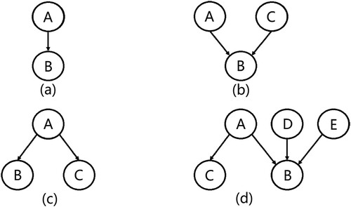
For the pattern in Figure 2(a), the communication cost between tasks A and B is ignored since both tasks involve only one single edge. The $\text{ran}{\text{k}}_{\text{spc}}(t_i)$ of this structure pattern is defined by (11) $\begin{array}{r}\text{ran}{\text{k}}_{\text{spc}}(t_i)=0\end{array}$(11) In (12) and (13), $|\text{ParentTask}(t_B)|$ is the number of parents for $t_B$ and $|\text{ChildrenTask}(t_A)|$ is the number of children for $t_A$. $|P|$ represents the total number of processors in the parallel system. (12) $\begin{array}{rl}\text{a}& =\text{ min}(|\text{ChildrenTask}(t_A)|,|P|)\end{array}$(12) (13) $\begin{array}{rl}b& =min(|\text{ParentTask}(t_B)|,|P|)\end{array}$(13) Figure 2(b) shows a join pattern among tasks. The $\text{ran}{\text{k}}_{\text{spc}}(t_i)$ of this structure pattern is defined by (14) $\begin{array}{r}\text{ran}{\text{k}}_{\text{spc}}(t_i)=\frac{b-1}{b}\times \overline{c_{A,B}}\end{array}$(14)

Figure 2(c) illustrates a fork pattern among tasks. The $\text{ran}{\text{k}}_{\text{spc}}(t_i)$ of this structure pattern is defined by (15) $\begin{array}{r}\text{ran}{\text{k}}_{\text{spc}}(t_i)=\frac{a-1}{a}\times \overline{c_{A,B}}\end{array}$(15) Figure 2(d) shows a more complicated mixed pattern of Figure 2(a–c). The $\text{ran}{\text{k}}_{\text{spc}}(t_i)$ of this structure pattern is defined by (16) $\begin{array}{r}\text{ran}{\text{k}}_{\text{spc}}(t_i)=\frac{a-1}{a}\times \frac{1}{a}\times \frac{b-1}{b}\times \overline{c_{A,B}}\end{array}$(16)

Based on the above definitions, the task rank in ResourceAwareEFT is calculated as follows. (17) $\begin{array}{r}\text{ran}{\text{k}}_{\text{STR}}(n_i)=\overline{w_i}+\underset{n_j\in \text{succ}(n_i)}{max}\left\{\begin{array}{c}\text{ran}{\text{k}}_{\text{SPC}}(n_j)\\ +\text{ran}{\text{k}}_{\text{STR}}(n_j)\end{array}\right\}\end{array}$(17)

D. IPPTS

Improved Predict Priority Task Scheduling (IPPTS) was proposed in (Djigal et al., 2021), which is the latest heuristic-based workflow scheduling algorithm. IPPTS maintains the same time complexity as previous well-known heuristic algorithms (Arabnejad & Barbosa, 2014; Topcuoglu et al., 2002; Xie et al., 2015), while outperforming them in terms of workflow execution makespan.

IPPTS is an improved version of PPTS (Djigal et al., 2019) based on a Predict Cost Matrix (PCM). The PCM equation (18) is similar to the OCT equation (8) in PEFT (Arabnejad & Barbosa, 2014), except that PCM takes into consideration the computation cost of the current task. (18) $\begin{array}{rl}& \text{PCM}(t_i,p_k)=\underset{t_j\in succ(t_i)}{max}\left[\underset{P_w\in P}{\text{min}}\{PCM(t_j,p_w)+w(t_i,p_w)+w(t_j,p_w)+\overline{c_{i,j}}\}\right],\\ & \overline{c_{i,j}}=0if{p}_w=p_k\end{array}$(18)

In the task prioritization phase, the average PCM value of each task is denoted by $\text{ran}{\text{k}}_{\text{PCM}}(t_i)$ and defined as follows. (19) $\begin{array}{r}\text{ran}{\text{k}}_{\text{PCM}}(t_i)=\frac{{\sum }_{k=1}^P\text{PCM}(t_i,p_k)}{|P|}\end{array}$(19) The rank of each task, denoted by $\text{Prank}(t_i)$, is computed by multiplying $\text{ran}{\text{k}}_{\text{PCM}}(t_i)$ with its out-degree $\text{outd}(t_i)$. (20) $\begin{array}{r}\text{Prank}(t_i)=\text{ran}{\text{k}}_{\text{PCM}}(t_i)\ast \text{outd}(t_i)\end{array}$(20)

In the processor selection phase, IPPTS uses Looking Ahead Earliest Finish Time $\text{Lhea}{\text{d}}_{\text{eft}}$ instead of the EFT mechanism (Sinnen, 2007). To compute $\text{Lhea}{\text{d}}_{\text{eft}}$, the Looking Head Exit Time LHET and EFT are involved. The $\text{LHET}(t_i,p_j)$ and $\text{Lhea}{\text{d}}_{\text{eft}}(t_i,p_j)$ are defined by (21) $\begin{array}{rl}\text{LHET}(t_i,p_j)& =\text{PCM}(t_i,p_j)-w(t_i,p_j)\end{array}$(21) (22) $\begin{array}{rl}\text{Lhea}{\text{d}}_{\text{eft}}(t_i,p_j)& =\text{EFT}(t_i,p_j)+\text{LHET}(t_i,p_j)\end{array}$(22)

E. Genetic Algorithm

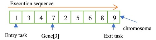
The Genetic Algorithm (GA, Srinivas & Patnaik, 1994) is a kind of evolutionary algorithm usually used for optimization problems. Previous works (Keshanchi et al., 2017; Sardaraz & Tahir, 2020; Xu et al., 2014) have applied GA to workflow scheduling, where a gene in a chromosome represents a task and the content of each chromosome is a possible task execution sequence for a specific workflow as shown in Figure 3. A population contains a pre-defined number of chromosomes representing various possible workflow execution schedules.

Figure 3. GA chromosome structure for workflow scheduling.

The approach proposed in (Keshanchi et al., 2017) starts with population initialization based on both heuristic and random chromosome generation. In the first step, heuristic chromosome generation is applied, where the schedules produced by heuristic workflow scheduling algorithms, such as HEFT-B (Topcuoglu et al., 2002), HEFT-T (Topcuoglu et al.,), and HEFT-L (Xu et al., 2014) are set as seed chromosomes. Then, in the second step of random chromosome generation, more chromosomes are randomly generated until the pre-defined population size is achieved.

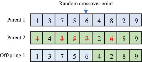
After population initialization, the GA approach will enter a loop of three essential operations, i.e. selection, crossover, and mutation, until a pre-defined termination condition is reached. In the selection phase, chromosomes will be randomly selected for performing the crossover and mutation operations on them. In the crossover phase, the elitist chromosome is the chromosome with the best fitness value, which will be marked and reserved with no update. Other chromosomes will be selected for the one-point crossover or two-point crossover operations to produce offsprings as new chromosomes. Figure 4 shows the one-point crossover operation used in (Keshanchi et al., 2017).

Figure 4. Single-point crossover operation.

The fitness of a chromosome is the resultant execution makespan of the schedule represented by it. In (Keshanchi et al., 2017), the execution makespan of a chromosome is calculated by applying the Earliest Finish Time (EFT, Sinnen, 2007) processor allocation policy to the task execution sequence represented in it. Therefore, a smaller value indicates better fitness.

In the mutation phase, chromosomes will be modified according to the mutation rule. For example, in (Xu et al., 2014) a task-swapping mutation was used, where a mutation point and a random point in a chromosome will be selected randomly for swapping the corresponding two tasks represented by the two genes if such swapping would not violate the inter-task dependence. The task-swapping mutation operation is shown in Figure 5.

Figure 5. Mutation operation – task swapping.

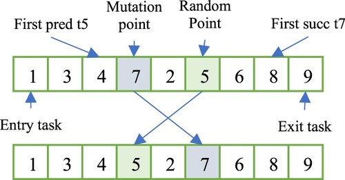
Figure 6. Mutation operation – processor allocation modification.

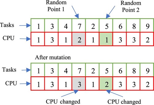
In our implementation of the GA-based workflow scheduling approach used in this paper for performance comparison with MCTS approaches, two chromosomes are used for representing a workflow execution schedule, one for task execution sequence and the other for processor allocation, as shown in Table 6. Therefore, when performing the mutation operation, in addition to task swapping, the processor allocation of the genes on the selected mutation and random points will also be changed randomly as shown in Table 6.

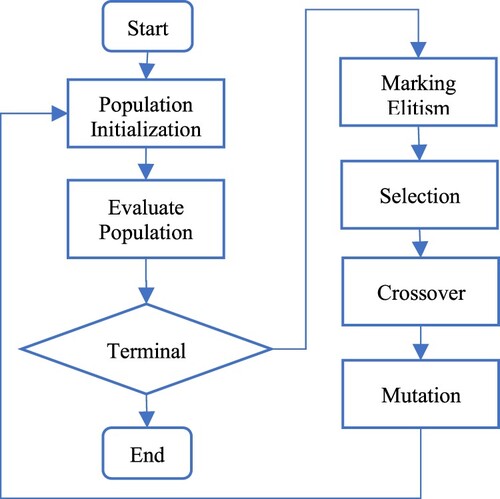
At the end of each iteration in the loop, the fitness value of each chromosome will be calculated. The termination condition of the loop is defined to be that all chromosomes have the same fitness. The elitist chromosome after the loop finishes will be returned as the best workflow execution schedule found by the GA approach. The entire GA workflow scheduling process is shown in Figure 7.

Figure 7. The process of GA-based workflow scheduling.

IV. Workflow scheduling based on MCTS

A. MCTS applied to workflow scheduling

Monte Carlo Tree Search (MCTS) is a heuristic searching algorithm consisting of four major steps. The entire search process of MCTS can be illustrated in Figure 8. When we apply MCST to workflow scheduling, each node in the MCTS tree represents a probable partial or complete schedule of a workflow to be executed on a set of processors. Nodes with complete schedules are called terminal nodes. The children of a node represent all possibilities of choosing an unscheduled ready task and allocating it to one of the processors. The root is a special node with an empty schedule where no tasks have been scheduled. MCTS starts with a single root node, and the tree gradually grows as illustrated in Figure 8 as the search process proceeds.

Figure 8. Monte Carlo Tree Search (Browne et al., 2012).

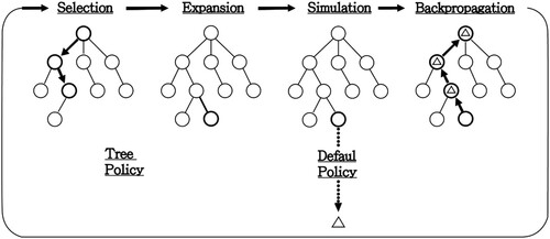
The four major steps in MCTS for workflow scheduling are described as follows.

1. Selection. Starting from the root node, a child is recursively selected at each visited node to proceed according to a selection policy until reaching a leaf node.

2. Expansion. If the selected leaf node in the previous step is not a terminal node, all its child nodes would be created and their visit counts and reward values are initialized. Then, one of the expanded child nodes is randomly selected for the following simulation step.

3. Simulation. Starting with the chosen node, a simulation strategy is used to extend the current partial schedule to a complete schedule and calculate the execution makespan of the resultant schedule.

4. Backpropagation. Updating the visit counts and reward values in the nodes on the path from the chosen node to the root node based on the complete schedule. The reward value in a node represents the shortest makespan ever found from the performed simulations going through it.

B. MCTS-BB

MCTS-BB is a recent MCTS approach for workflow scheduling, which is equipped with a pruning method based on the branch-and-bound concept. The proposed pruning method is used to prevent MCTS from exploring some unpromising subtrees. Tree pruning is performed in the selection step, where the selected maximum UCT node will be marked as disabled if it meets the pruning criterion, to prevent it from further exploration. Once tree pruning occurs, the search process would start over again from the root node. Otherwise, the search process will continue as shown in Algorithm 1.

Table

Algorithm 1: MCTS-BB Pruning

Input: selected node n with maximum uct value

Variable: β as current best makespan ever found

1. Calculate Mark(n)

2. if Mark(n) > β

3.   mark node n as disabled

4.   cut off n’s children nodes

5.   return selection(root)

6. else

7.   return n // continue to selection step

8. end if

The pruning criterion is that the estimated makespan going through the selected node exceeds the current shortest execution makespan ever found, i.e. β in Algorithm 1. The estimated makespan M of the selected node is calculated by summing up the makespan of the current partial schedule and the length of the critical path CP_last among the unscheduled tasks as follows, where $\underset{p_j\in P}{max}\{\text{avail}[j]\}$ is the makespan of the current partial schedule. (23) $\begin{array}{r}M=\underset{p_j\in P}{max}\{\text{avail}[j]\}+\sum _{n_i\in C{P}_{last}}min{\{w_{i,j}\}}_{p_j\in P}\end{array}$(23) The critical path in equation (18), i.e. $\text{C}{\text{P}}_{\text{last}}$, could be determined by calculating the sum of upward rank, i.e. equation (7), and downward rank, i.e. equation (24), for each task. The tasks with the largest rank’s sum belong to the critical paths. (24) $\begin{array}{r}\text{ran}{\text{k}}_d(n_i)=+\underset{n_i\in pred(n_i)}{max}\{\overline{c_{i,j}}+\overline{w_i}+\text{ran}{\text{k}}_u(n_i)\}\end{array}$(24)

Since the entire MCTS process is usually controlled by a pre-defined total search time or simulation count limit, a good pruning algorithm can avoid wasting time on exploring those nodes which look unlikely to lead to a better schedule than ever found, and thus increase the probability of finding a better schedule within the same search time limit. However, on the other hand, a flawed pruning algorithm might run the risk of missing some nodes which actually would result in better schedules. The experimental results in (Liu et al., 2019) showed that MCTS-BB achieved worse makespan than MCTS on average, indicating that the pruning algorithm adopted in MCTS-BB leaves room for further improvement.

V. Our improved MCTS approach for workflow scheduling

This section presents the methods we propose to improve the MCTS process for workflow scheduling.

A. Pre-calculated upper bound of makespan

The first improvement we made is a new pruning algorithm utilizing existing workflow scheduling heuristic algorithms (Arabnejad & Barbosa, 2014; Chen & Huang, 2019; Topcuoglu et al., 2002, July; Djigal et al., 2021). Instead of the critical path length of unscheduled tasks used in MCTS-BB, our approach adopts the minimum makespan value achieved by HEFT, PEFT, ResourceAwareEFT, CPOP, IPPTS as the initial upper bound before searching for the best schedule via MCTS i.e. lines 1–2 in Algorithm 2.

B. Estimated makespan of unscheduled tasks

Instead of the critical path length used in MCTS-BB, our approach estimates the minimum makespan of all possible schedules extended from a node allocated on a specific processor by adding up the node’s EFT and the summation of all its successors’ shortest required execution time divided by the number of processors in the system, i.e. equation (25). Based on such makespan estimation, our new pruning algorithm could avoid the risk of disabling promising nodes for further exploration. (25) $\begin{array}{r}M=\text{EFT}(n_i,p_j)+\frac{{\sum }_{n_k\in Al{l}_{Succ(n_i)}}\text{mi}{\text{n}}_{p_j}ϵP\{w_{k,j}\}}{|P|}\end{array}$(25)

C. Node selection policy

At the selection step, the UCT equation in (Kocsis & Szepesvári, 2006) is the most widely used node selection policy. In (Liu et al., 2019), a variant of the original UCT equation as shown in equation (26) was used in the selection step, where $Q(s,a)$ and $U(s,a)$ represent the reward value and the visit count of the current tree node, respectively. In this paper, we evaluate other possible node selection policies, which will be described in the performance evaluation section. $\begin{array}{rl}\text{UCT}(s,a)& =\text{argmax}(Q(s,a)+U(s,a))\end{array}$ (26) $\begin{array}{rl}U(s,a)& =\text{Cpuct}\frac{\sqrt{{\sum }_{b}N(s,b)}}{1+N(s,a)}\end{array}$(26)

D. Node expansion strategy

At the expansion step, we propose a new heuristic strategy for guiding the expansion aiming to improve the search effectiveness. In MCTS-BB, a random expansion policy was used. In this paper, we propose and evaluate three new expansion policies based on a task’s upward rank (Topcuoglu et al., 2002), OCT-rank (Arabnejad & Barbosa, 2014) and STR-rank (Chen & Huang, 2019, July), respectively. The task with the highest rank value would be chosen for expansion as described in line 10 of Algorithm.

E. Simulation strategy

At the simulation step, we propose a new strategy aiming to improve the simulation effectiveness. In MCTS-BB, a random simulation strategy was used, which repeatedly selects an unscheduled task randomly until all tasks are scheduled. Regarding processor allocation, in (Liu et al., 2019), a probability parameter $R_{\text{threshold}}$ was set, and a task has $R_{\text{threshold}}$ probability to be allocated randomly and (1−$R_{\text{threshold}}$) probability to be allocated to a processor chosen by the EFT mechanism (Sinnen, 2007). In this paper, we propose and evaluate three policies for selecting unscheduled tasks based on HEFT, $\text{OC}{\text{T}}_{\text{rank}}+\text{EFT}$ and ResourceAwareEFT, respectively. We also adopt the $R_{\text{threshold}}$ concept for processor allocation. In the experiments, we will evaluate the effectiveness of different values for $R_{\text{threshold}}$. The overall process of our improved MCTS approach and the major steps in it are presented in the following Algorithm 2 to Algorithm.

Table

Algorithm 2: Improved MCTS for workflow scheduling

Input: A workflow to be scheduled

Output: The best schedule found by MCTS

1. Schedule the workflow by heuristic algorithms (HEFT, ResourceAwareEFT, PEFT, CPOP, IPPTS)

2. Adopt the best one among the above results as the upper bound for makespan

3. Initialize the tree and create the root node nroot

4. Compute required task rank values

5. while simulation_count_limit is not reached do

6.  nselected = selection(nroot) //Algorithm 3

7.  nexpanded = expansion(nselected) //Algorithm 4

8.  simulation(nexpanded) //Algorithm 5

9.  backpropagation(nexpanded)

10. end while

11. return the best makespan ever found

Table

Algorithm 3: workflow_simulate

Input:

The node where simulation starts

The specified workflow scheduling algorithm

Probability threshold used for processor allocation

Output: makespan

1. Initialize list < Cpu, Event > schedule for all scheduled task, and put them into the list

2. Schedule remaining unscheduled tasks by the specified workflow scheduling algorithm

3. return resultant makespan

Table

Algorithm 4: Node selection

Input: The root node

Output: The selected node

1. max_uct = negative_infinitive

2. max_uct_node = null

3. while (True)

4. if children_size(node) = 0 then

5.  return node

6. end if

7. foreach children(node) as child_node do

8.   if is_disabled(child_node) then

9.   continue

10.  end if

11.  if child_nodemin_makespan > upper_bound then

12.   disable(child_node)

13.  else if child_node.uct > max_uct then

14.   max_uct = child_node.uct

15.   max_uct_node = child_node

16.  end if

17. end foreach

18. if max_uct_node = null then

19.  disable(node)

20.  return selection(parent_node(node))

21. end if

22. node = max_uct_node

23. end while

Table

Algorithm 5: Node expansion

Input: The selected node

Output: The node where simulation starts

1. if node.event = null or node.task = exist_task then

2.  return node

3. end if

4. ready_tasks = get_ready_task(node)

5. foreach (get_cpu_list() as cpu) do

6.  foreach (ready_tasks as task) do

7.   node.add_child(new Node(cpu, task))

8.  end foreach

9. end foreach

10. return highest_task_rank_child_node (node)

Table

Algorithm 6: Simulation

Input: The node chosen at the expansion step

1. if task(node) = exist_task then

2.  makespan = calculate_finish_time(node)

3.  best_makespan = max(makespan, best_makespan)

4.  disable(node)

5.  return

6. end if

7. makespan = workflow_simulate(node, simulate algorithm, threshold)

8. best_makespan  = max(makespan, best_makespan)

9. update node.min_makespan

10. return

VI. Performance evaluation

This section presents the performance evaluation of the proposed MCTS-based workflow scheduling approach, compared to well-known previous methods.

A. Experiment setup and performance metrics

There are several toolkits available for generating various workflow structures to be used in evaluating workflow scheduling algorithms. WorkflowGenerator (Juve, 2014) is a toolkit developed in the Pegasus project, which could generate various workflow structures of real-world applications, including Cybershake, Montage, Epigenomics, Insprial and Sipht, described in the Pegasus DAX format. DAGGEN (Suter, 2015) is a software tool developed by Suter et al for generating a wide range of random workflow structures based on user input parameters such as the number of tasks, fatness and density of DAG. It is useful for evaluating workflow scheduling algorithms. DAGGEN supports both dot and text formats. Both toolkits were used in the following experiments.

The experiments were conducted on WorkflowSim (Chen, 2015; Chen & Deelman, 2012), which is a workflow scheduling simulation toolkit developed by Chen based on CloudSim (Calheiros et al., 2011). We wrote a simple program to convert the dot format files produced by DAGGEN into the XML input format used by WorflowSim.

DAGGEN has the following parameters to set for generating workflows of various structures and properties.

• n: the number of tasks in a workflow

• fat: regarding the DAG shape, ranging in [0,1]. A value close to 1 means a fat DAG with greater parallelism, while a value close to 0 indicates a thin DAG with less parallelism.

• density: controlling the inter-dependence of tasks in adjacent levels of a DAG.

• regularity: controlling the distribution of tasks between different levels of a DAG.

• jump: regarding the allowed distance between a task and its parent in terms of levels in a DAG.

• ccr: the ratio of communication cost to computation cost.

Table 1 lists the parameter values used in the following experiments for generating workflows of various structures.

Table 1. Parameter values for DAG generation.

n	= [20, 40, 60, 80, 100]
fat	= [0.1, 0.4, 0.6]
density	= [0.2, 0.4]
regularity	= [0.4, 0.8]
jump	= [1, 2, 4]
ccr	= [0.1, 1.0, 10.0]

In the experiments, we also used WorkflowGenerator to generate the real-world applications’ workflow structures, such as CyberShake, Epigenomics, and Montage, to evaluate the performance of different workflow scheduling algorithms.

Table 2 shows the parameter values used in the GA-based workflow scheduling method in the following experiments.

Table 2. Parameter values for GA-based method.

Parameters (Keshanchi et al., 2017)	Values
population size	4 times to task list size
crossover probability	75%
Task mutation prob.	15%
CPU mutation prob.	15%
termination condition	when no chromosomes achieve better makespan over 5 iterations.

The following performance metrics were used in our simulation experiments for performance evaluation.

• Normalized Makespan. Equation (27) is used to normalize the makespan in comparing the performance of different workflow scheduling algorithms. The range of the normalized makespan is between 0 and 1. A normalized makespan close to 1 means a relatively worse performance, while a value near 0 indicates superior performance. (27) $\begin{array}{r}\mathrm{makespa}{\mathrm{n}}^{\mathrm{\prime }}=\frac{\text{makespan}-\text{makespa}{\text{n}}_{\text{min}}}{\text{makespa}{\text{n}}_{\text{max}}-\text{makespa}{\text{n}}_{\text{min}}}\end{array}$(27)

• Schedule Length Ratio (SLR). The definition of SLR, as shown in equation (28), is the makespan divided by the summation of the shortest required execution time of all tasks on the critical path in the workflow. SLR is the resultant makespan normalized to the lower bound. (28) $\begin{array}{r}\text{SLR}=\frac{\text{makespan}}{\sum n_i\in \text{ C}{\text{P}}_{\text{last}}\text{mi}{\text{n}}_{p_j}\in P\{w_{i,j}\}}\end{array}$(28)

• Speedup. The definition of speedup is the minimum cumulative computation cost of all tasks in a workflow divided by parallel execution time, i.e. makespan, as shown in equation (29). (29) $\begin{array}{r}\text{Speedup}=\frac{\sum n_i\in N\text{mi}{\text{n}}_{p_j}ϵP\{w_{i,j}\}}{\text{makespan}}\end{array}$(29)

• Algorithm Run Time. This is the measure used to compare the computational overheads of different workflow scheduling algorithms.

B. Experimental results and discussions

This section presents the simulation experiments conducted to evaluate the pruning algorithm and guided heuristics proposed in this paper. Four sets of experiments were conducted to evaluate different types of pruning algorithms and guiding heuristics. We conducted the experiments for the simulation strategies first to determine the best $R_{\text{threshold}}$ for use in other sets of experiments. In each experiment, MCTS would stop when the simulation count reaches 100,000. Equation (25) was applied in all cases except for MCTS-BB. Workflows of three different CCR values, 0.1, 1, and 10, were used as input data. MCTS-1111 represents the standard MCTS algorithm.

C. Experiment set 1: simulation strategies

To determine the best simulation strategy in MCTS and the corresponding $R_{\text{threshold}}$, we conducted experiments for the random policy in MCTS-BB and the simulation policies guided by HEFT, $\text{OC}{\text{T}}_{\text{rank}}+\text{EFT}$, and ResourceAwareEFT with $R_{\text{threshold}}$ set to 0, 20 and 30. Tables 3–5 show the experimental results.

• MCTS-1111-0: The simulation policy in MCTS-BB, $R_{\text{threshold}}$ is set to 0.

• MCTS-1111-20: The simulation policy in MCTS-BB, $R_{\text{threshold}}$ is set to 20.

• MCTS-1111-30: The simulation policy in MCTS-BB, $R_{\text{threshold}}$ is set to 30.

• MCTS-1112-0: The simulation policy guided by HEFT, $R_{\text{threshold}}$ is set to 0.

• MCTS-1112-20: The simulation policy guided by HEFT, $R_{\text{threshold}}$ is set to 20.

• MCTS-1112-30: The simulation policy guided by HEFT, $R_{\text{threshold}}$ is set to 30.

• MCTS-1113-0: The simulation policy guided by $\text{OC}{\text{T}}_{\text{rank}}+\text{EFT}$, $R_{\text{threshold}}$ is set to 0.

• MCTS-1113-20: The simulation policy guided by $\text{OC}{\text{T}}_{\text{rank}}+\text{EFT}$, $R_{\text{threshold}}$ is set to 20.

• MCTS-1113-30: The simulation policy guided by $\text{OC}{\text{T}}_{\text{rank}}+\text{EFT}$, $R_{\text{threshold}}$ is set to 30.

• MCTS-1114-0: The simulation policy guided by ResourceAwareEFT, $R_{\text{threshold}}$ is set to 0.

• MCTS-1114-20: The simulation policy guided by ResourceAwareEFT, $R_{\text{threshold}}$ is set to 20.

• MCTS-1114-30: The simulation policy guided by ResourceAwareEFT, $R_{\text{threshold}}$ is set to 30.

Table 3. Experiment 1: Normalized makespan for different workflow sizes – CCR = 0.1.

	Algorithms (Prefix : MCTS_)
Tasks	1111-0	1111-20	1111-30	1112-0	1112-20	1112-30	1113-0	1113-20	1113-30	1114-0	1114-20	1114-30
20	0.410	0.682	0.702	0.012	0.008	0.016	0.147	0.018	0.052	0.020	0.007*	0.018
40	0.545	0.593	0.730	0.160	0.057*	0.097	0.373	0.108	0.140	0.175	0.084	0.103
60	0.680	0.584	0.660	0.190	0.095*	0.146	0.333	0.153	0.153	0.204	0.116	0.192
80	0.799	0.605	0.620	0.114	0.111*	0.133	0.243	0.195	0.214	0.134	0.124	0.143
100	0.804	0.630	0.555	0.121	0.100*	0.146	0.224	0.195	0.214	0.130	0.140	0.152
average	0.647	0.619	0.654	0.119	0.074*	0.108	0.264	0.134	0.155	0.133	0.094	0.121

Table 4. Experiment 1: Normalized makespan for different workflow sizes – CCR = 1.

CCR1.0	Algorithms (Prefix : MCTS-)
Tasks	1111-0	1111-20	1111-30	1112-0	1112-20	1112-30	1113-0	1113-20	1113-30	1114-0	1114-20	1114-30
20	0.627	0.647	0.723	0.113	0.046	0.066	0.227	0.083	0.101	0.077	0.024*	0.077
40	0.788	0.764	0.709	0.059	0.043	0.094	0.122	0.087	0.135	0.077	0.037*	0.077
60	0.811	0.857	0.867	0.019*	0.038	0.084	0.076	0.069	0.139	0.098	0.043	0.098
80	0.800	0.906	0.950	0.013*	0.038	0.104	0.083	0.083	0.144	0.112	0.041	0.112
100	0.839	0.925	0.982	0.009*	0.049	0.123	0.069	0.095	0.159	0.116	0.056	0.116
Average	0.773	0.820	0.846	0.042	0.043	0.094	0.115	0.084	0.136	0.096	0.040*	0.096

Table 5. Experiment 1: Normalized makespan for different workflow sizes – CCR = 10.

CCR10	Algorithms (Prefix : MCTS-)
Tasks	1111-0	1111-20	1111-30	1112-0	1112-20	1112-30	1113-0	1113-20	1113-30	1114-0	1114-20	1114-30
20	0.752	0.683	0.709	0.227	0.124	0.191	0.274	0.169	0.210	0.156	0.105*	0.156
40	0.554	0.814	0.987	0.111	0.095	0.190	0.114	0.114	0.252	0.194	0.067*	0.194
60	0.523	0.799	0.999	0.078*	0.084	0.212	0.085	0.114	0.265	0.191	0.096	0.191
80	0.525	0.818	0.996	0.037*	0.076	0.224	0.059	0.140	0.254	0.206	0.088	0.206
100	0.537	0.836	0.992	0.024*	0.109	0.242	0.071	0.150	0.282	0.249	0.125	0.249
Average	0.578	0.790	0.937	0.095*	0.098	0.212	0.121	0.137	0.253	0.199	0.096	0.199

According to Table 6, on average the simulation policy guided by HEFT with $R_{\text{threshold}}$ set to 20% (MCTS-1112-20) significantly achieved the best performance among all simulation policies and configurations. In contrast, the random simulation policy (MCTS-1111) used in MCTS-BB results in the worst performance. Moreover, the heuristic simulation policies (MCTS-1112, MCTS-1113, MCTS-114) with $R_{\text{threshold}}=0$ result in poorer performance compared to $R_{\text{threshold}}=20$ and $R_{\text{threshold}}=30$, indicating the importance of introducing randomness in the simulation step. Therefore, we used $R_{\text{threshold}}=20\mathrm{\%}$ in the following experiments.

Table 6. Experiment 1: Normalized makespan for overall performance.

	Algorithms (Prefix: MCTS-)
CCR	1111-0	1111-20	1111-30	1112-0	1112-20	1112-30	1113-0	1113-20	1113-30	1114-0	1114-20	1114-30
0.1	0.647	0.619	0.654	0.119	0.074*	0.108	0.264	0.134	0.155	0.133	0.094	0.121
1.0	0.773	0.820	0.846	0.042	0.043	0.094	0.115	0.084	0.136	0.096	0.040*	0.096
10.0	0.578	0.790	0.937	0.095*	0.098	0.212	0.121	0.137	0.253	0.199	0.096	0.199
Average	0.666	0.743	0.812	0.086	0.072*	0.138	0.167	0.118	0.181	0.143	0.077	0.139

D. Experiment set 2: pruning methods

This section evaluates the performance of our pruning method.

• MCTS-1111: No pruning performed.

• MCTS-1211: Our pruning method in section VI.

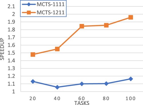
Figures 9–11 show the experimental results in terms of speedup for workflows of different CCR values, respectively. Our pruning method shows the greatest potential for performance improvement in all cases. Moreover, the performance improvement is even large for large-scale workflows.

Figure 9. Experiment 2: Speedup comparison – CCR = 0.1.

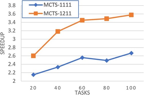
Figure 10. Experiment 2: Speedup comparison – CCR = 1.

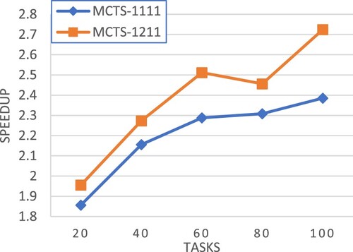
Figure 11. Experiment 2: Speedup comparison – CCR = 10.

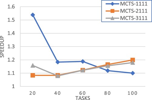
E. Experiment set 3: selection policies

This section evaluates different selection policies.

• MCTS-1111: using equation (26) in the selection step, $\text{Cpuct}=-15$. $Q(s,a)$ in MCTS-BB (Liu et al., 2019) is defined as (30) $\begin{array}{r}Q(s,a)=Q(s,a)+\text{makespan}(s,a)\end{array}$(30)

• MCTS-2111: similar to MCTS-1111 except that the reciprocal of makespan is used for $Q(s,a)$. (31) $\begin{array}{r}Q(s,a)=\frac{1}{\text{makespan}(s,a)}\end{array}$(31)

• MCTS_3111: using the traditional UCT equation (Kocsis & Szepesvári, 2006) in the selection step, $\text{Cpuct}=-15$. $Q(s,a)$ is also set to the reciprocal of makespan. (32) $\begin{array}{r}U(s,a)=\text{Cpuct}\sqrt{\frac{{\sum }_{b}N(s,b)}{N(s,a)}}\end{array}$(32)

Figures 12–14 show the experimental results. MCTS-1111, using the UCT equation (26), achieves the best performance in Figure 12. MCTS-2111 using the reciprocal of makespan and MCTS-3111 using the traditional UCT equation (Kocsis & Szepesvári, 2006) achieve better performance for workflows of larger sizes, e.g. 60 and 80 tasks, and CCR values, e.g. 1 and 10, as shown in Figures 13 and 14.

Figure 12. Experiment set 3: Speedup comparison – CCR = 0.1.

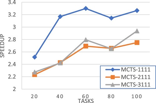
Figure 13. Experiment set 3 speedup comparison – CCR = 1.

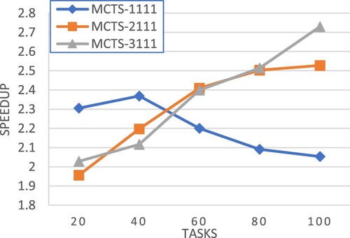
Figure 14. Experiment set 3: Speedup comparison – CCR = 10.

F. Experiment set 4: expansion polices

This section presents experimental results evaluating different expansion policies.

• MCTS-1111: the random policy in MCTS-BB.

• MCTS-1121: using the upward rank in HEFT to choose a node for expansion. The task with the highest rank value would be chosen.

• MCTS-1131: using the OCT-rank in PEFT to choose a node for expansion. The task with the highest rank value would be chosen.

• MCTS-1141: using the STR-rank in ResourceAwareEFT to choose a node for expansion. The task with the highest rank value would be chosen.

Table 7–10 present the experimental results. In general, the random expansion policy (MCTS-1111) achieves the best performance for workflows with a smaller CCR value or a larger CCR value, e.g. CCR =0.1 and CCR = 10 as shown in Tables 7 and 9. On the other hand, the expansion policy based on the upward rank (MCTS-1121) outperforms the others for workflows of a medium CCR value, e.g. 1 as shown in Table 1. Considering all CCR values, on average the random expansion policy (MCTS-1111) achieved the best performance as shown in Table 10.

Table 7. Experiment 4: Normalized makespan comparison – CCR = 0.1.

CCR0.1	Algorithms (Prefix : MCTS-)
Tasks	1111	1121	1131	1141
20	0.310*	0.438	0.566	0.410
40	0.444*	0.595	0.471	0.480
60	0.390*	0.568	0.558	0.561
80	0.501	0.430*	0.568	0.495
100	0.467*	0.479	0.522	0.477
Average	0.422*	0.502	0.537	0.485

Table 8. Experiment 4: Normalized makespan comparison – CCR = 1.

CCR1.0	Algorithms (Prefix : MCTS-)
Tasks	1111	1121	1131	1141
20	0.381	0.500	0.344*	0.536
40	0.491	0.404*	0.475	0.496
60	0.573	0.469	0.450*	0.583
80	0.585	0.453	0.605	0.380*
100	0.687	0.415*	0.562	0.489
Average	0.543	0.448*	0.487	0.497

Table 9. Experiment 4: Normalized makespan comparison – CCR = 10.

CCR10.0	Algorithms (Prefix : MCTS-)
Tasks	1111	1121	1131	1141
20	0.466	0.516	0.448*	0.485
40	0.407*	0.557	0.546	0.624
60	0.423*	0.585	0.573	0.431
80	0.395*	0.564	0.618	0.497
100	0.519	0.376*	0.593	0.643
Average	0.442*	0.519	0.555	0.536

Table 10. Experiment 4: Overall normalized makespan comparison.

	Algorithms (Prefix: MCTS-)
CCR	1111	1121	1131	1141
0.1	0.422*	0.502	0.537	0.485
1.0	0.543	0.448*	0.487	0.497
10.0	0.442*	0.519	0.555	0.536
Average	0.469*	0.490	0.527	0.506

VII. Overall performance evaluation

In this section, we present the overall performance evaluation of our improved MCTS approach for workflow scheduling consisting of the proposed policies described in the previous sections. Based on the previous experimental results, the following three variants of our approach were compared to the standard MCTS approach (MCTS-1111), MCTS-BB, IPPTS, and the GA-based workflow scheduling method in the following experiments. All the three variants adopt our pruning method and the same simulation policy guided by HEFT but differ in the selection and expansion policies.

• MCTS-1212: using equation (26) in the selection policy and using the random node expansion policy.

• MCTS-3212: using equation (31) in the selection policy and using the random node expansion policy.

• MCTS-3222: using equation (32) in the selection policy and using the node expansion policy based on the upward rank in HEFT.

The following presents the performance evaluation of our MCTS workflow scheduling approaches compared to the standard MCTS method and MCTS-BB in a homogenous computing environment. Tables 11–13 show the experimental results for workflows of different CCR values, respectively. In general, our approaches outperform the standard MCTS method and MCTS-BB. MCTS-1222 achieves the best performance across all the three CCR values.

Table 11. Normalized makespan – CCR = 0.1.

CCR0.1	Algorithms (Prefix: MCTS-)
Tasks	1111	1212	1222	3212	3222	BB
20	0.750	0.000*	0.037	0.037	0.035	0.567
40	0.763	0.073	0.048*	0.179	0.184	0.641
60	0.768	0.086	0.052	0.242	0.256	0.752
80	0.819	0.103*	0.109	0.168	0.191	0.758
100	0.794	0.143	0.129*	0.185	0.209	0.777
Average	0.779	0.081	0.075*	0.162	0.175	0.699

Table 12. Normalized makespan – CCR = 1.

CCR1	Algorithms (Prefix: MCTS-)
Tasks	1111	1212	1222	3212	3222	BB
20	0.713	0.022	0.021*	0.149	0.104	0.572
40	0.866	0.024	0.018*	0.062	0.072	0.834
60	0.956	0.003*	0.006	0.026	0.029	0.937
80	0.979	0.004	0.004*	0.012	0.010	0.952
100	0.970	0.008*	0.012	0.013	0.022	0.968
Average	0.897	0.012	0.012*	0.052	0.047	0.852

Table 13. Normalized makespan – CCR = 10.

CCR10	Algorithms (Prefix: MCTS-)
Tasks	1111	1212	1222	3212	3222	BB
20	0.688	0.106	0.100*	0.541	0.358	0.480
40	0.971	0.081	0.083	0.235	0.124	0.858
60	0.953	0.053	0.041*	0.144	0.063	0.917
80	0.966	0.073	0.084	0.127	0.022*	0.955
100	0.967	0.079	0.079	0.106	0.020*	0.970
Average	0.909	0.078	0.077*	0.230	0.117	0.836

This following presents the performance evaluation of our MCTS workflow scheduling approaches in a parallel computing environment of speed-heterogeneous processors. Table 14 shows the performance comparison in terms of normalized makespan. Figures 15 and 16 compares different scheduling approaches in terms of SLR, while Figure 17 makes the comparison in terms of speedup. Figure 18 compares the algorithm runtime of different approaches. All the above performance comparisons were made on synthetic workflows generated by DAGGEN.

Figure 15. Average SLR for workflow size 20, 40, 60.

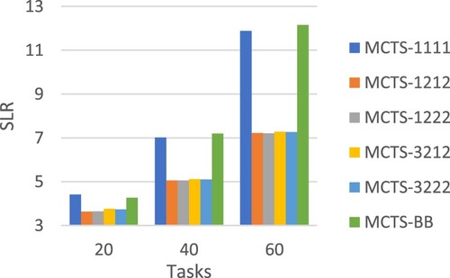
Figure 16. Average SLR for workflow size 80, 100.

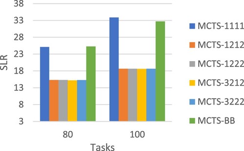
Figure 17. Average speedup for different workflow sizes.

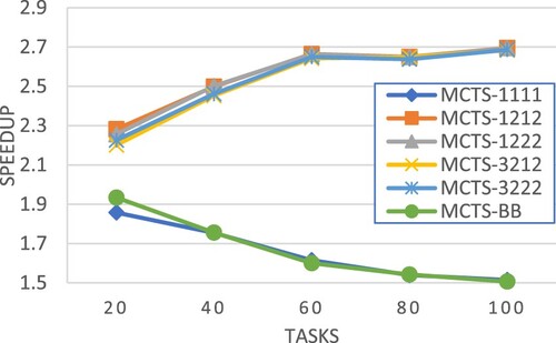
Figure 18. Average runtime of different scheduling approaches.

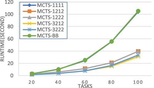
Table 14. Normalized makespan.

	Algorithms (Prefix: MCTS-)
Tasks	1111	1212	1222	3212	3222	BB
20	0.831	0.049	0.047*	0.167	0.140	0.714
40	0.840	0.010*	0.011	0.031	0.028	0.826
60	0.953	0.004	0.004	0.017	0.012	0.898
80	0.974	0.006	0.007	0.006*	0.008	0.959
100	0.979	0.005	0.005*	0.009	0.008	0.960
Average	0.915	0.015	0.015*	0.046	0.039	0.871

In terms of normalized makespan, MCTS-1222 achieved the best average performance. MCTS-1222 also performed very well in terms of SLR, speedup and runtime as shown in Figures 15–18.

Table 15 evaluates the scheduling approaches using workflow structures of real-world applications generated by WorkflowGenerator. On average, MCTS-1222 achieved the best performance. Figures 19–Figure 23 show the detailed performance comparison for each specific real-world workflow application structure, where each scheduling approach exhibited superiority over others in different scenarios.

Figure 19. Average speedup of CyberShake workflow.

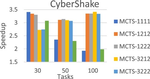
Figure 20. Average speedup of Epigenomics workflow.

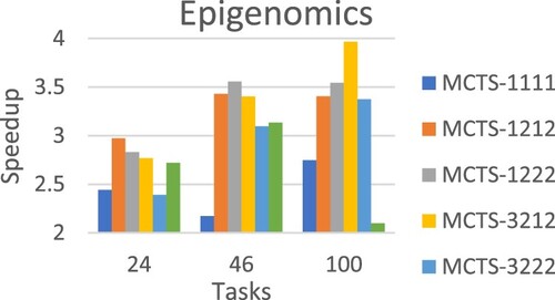
Figure 21. Average speedup of Inspiral workflow.

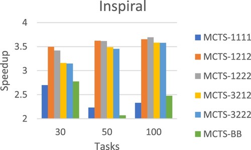
Figure 22. Average speedup of Montage workflow.

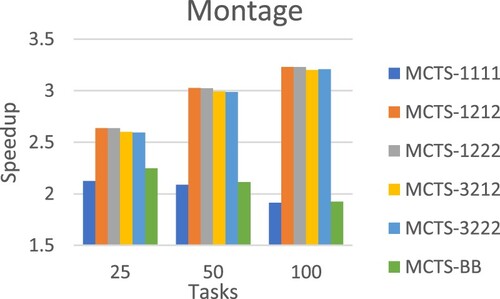
Figure 23. Average speedup of Sipht workflow.

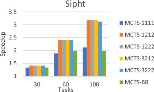
Table 15. Normalized makespan of real-world workflow applications.

	Algorithms (Prefix: MCTS-)
Workflow	Size	1111	1212	1222	3212	3222	BB
CyberShake	30	0.173	0.133*	0.141	0.986	0.939	0.478
	50	0.876	0.043	0.018*	0.061	0.077	0.944
	100	0.977	0.033	0.033	0.012*	0.037	0.912
Epigenomics	24	0.615	0.103*	0.135	0.207	0.581	0.405
	46	0.800	0.107	0.076*	0.128	0.220	0.391
	100	0.506	0.150	0.109	0.037*	0.161	0.918
Inspiral	30	0.851	0.036*	0.092	0.308	0.326	0.730
	50	0.835	0.032	0.026*	0.075	0.088	0.978
	100	0.894	0.017	0.005*	0.047	0.049	0.778
Montage	25	1.000	0.009*	0.009	0.071	0.079	0.736
	50	0.980	0.003*	0.005	0.029	0.032	0.940
	100	0.979	0.001*	0.002	0.015	0.011	0.966
Sipht	30	0.988	0.005	0.004	0.006	0.001*	0.974
	60	0.848	0.002	0.001*	0.010	0.009	0.698
	100	0.828	0.013	0.004*	0.010	0.040	1.000
Average		0.810	0.046	0.044*	0.134	0.177	0.790

In (Liu et al., 2019), MCTS-based methods were only compared to heuristic workflow scheduling algorithms. In the following, we compare the proposed MCTS-based method to both major categories of workflow scheduling approaches, including a GA-based method (Keshanchi et al., 2017) and the latest heuristic based algorithm IPPTS (Djigal et al., 2021), which has been shown to outperform well known previous heuristic algorithms such as HEFT and PEFT.

Trying to make a fair comparison between MCTS and GA, we first record the total number of generated chromosomes when the GA-based approach converges. Then, we let the MCTS-based scheduling methods stop when its simulation count reaches the recorded number. To conduct a comprehensive comparison, we also evaluated the performance of the MCTS-based approach with different simulation counts, set to specific ratios of the recorded number for the GA-based method. For example, the GA-based method generated 10,000 chromosomes for a specific input workflow DAG-01.dot. Then, we would evaluate MCTS-1222 with different simulation counts ranging [10,000*1 = 10,000, 10,000*0.1 = 1000, 10,000*0.01 = 100, 10,000*0.001 = 10]. The average recorded number for the GA-based method and the corresponding simulation counts for the MCTS-based approach is shown in Table 16.

Table 16. Average simulation counts for different workflow sizes.

	Ratio
Task	GA	0.1	0.01	0.001
20	24,792	2479	248	26
40	120,274	12,027	1203	120
60	290,661	29,066	2907	291
80	532,919	53,292	5329	533
100	836,507	83,651	8365	837

Figures 24 and 25 present the performance comparison in terms of average speedup. It is obvious that for smaller workflows, e.g. 20 tasks in Figure 24, our approach MCTS-1222 outperforms all the others even using a less simulation count, 1% of the total number of generated chromosomes in the GA-based method. The experimental results also show that more simulations could effectively improve the workflow execution schedules produced by the MCTS-based approach. Figures 26 and 27 compare the scheduling time required for different methods. It is clear that in general MCTS-based approaches would take a longer time to produce the schedules, and the time increases largely as the workflow size grows. This points out an important future research topic for MCTS-based workflow scheduling, developing efficient mechanisms to reduce the required search time.

Figure 24. Average speedup of workflow size 20 and 40.

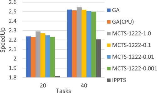
Figure 25. Average speedup of workflow size 60, 80 and 100.

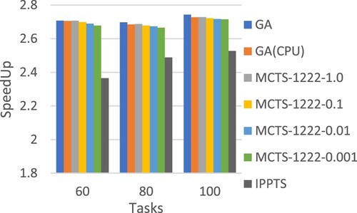
Figure 26. Average runtime of different scheduling approaches.

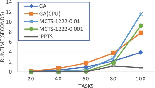
Figure 27. Average runtime of MCTS-1222 in different simulation limit.

According to the above experimental results, our improved MCTS-based workflow scheduling approach not only outperforms MCTS-BB (Liu et al., 2019) in terms of schedule quality but also requires less scheduling time. In the following, we present the experimental analysis of the advantage of our approach. Benefitting from the new pruning method and other proposed mechanisms for the selection, expansion, and simulation steps in MCTS, Our approach could disable more unpromising nodes than MCTS-BB as shown in Figure 28.

Figure 28. Average number of disabled nodes.

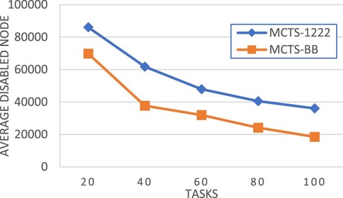
Table 17 takes a specific input workflow, n-0040-ccr-1.0-fat-0.8-regular-0.2-density-0.8-jump-2-000001.dot, for a case study, comparing the workflow execution makespan, required scheduling time and resultant MCTS trees between MCTS-BB and our approach. In this case, our approach produces a better schedule of shorter makespan while spending less time in scheduling. Table 17 shows that our approach grows a smaller MCTS tree and disables more nodes in the tree, resulting in superiority over MCTS-BB. Figure 29 compares the MCTS tree properties of our approach and MCTS-BB in terms of the number of nodes at different tree depths. The comparison shows that our approach builds an MCTS tree of more narrow widths at the top levels, demonstrating the advantage of focusing on promising directions quickly.

Figure 29. The node distribution of MCTS-1222 and MCTS-BB.

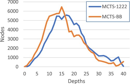
Table 17. Comparison of MCTS tree structure.

	Scheduling time	Makespan	Tree nodes	Disabled nodes
MCTS-1222	8.667099	1524	106,200	29,163
MCTS-BB	14.32798	1937	107,775	11,960

VIII. Conclusion and future work

Monte Carlo Tree Search (MCTS) is a promising direction for workflow scheduling but was less explored in previous studies. In this paper, we present and evaluate several new mechanisms to further improve the effectiveness of MCTS when applied to workflow scheduling, including a new pruning algorithm and new heuristics for guiding the selection, expansion and simulation steps in MCTS. Performance evaluation was conducted with simulation experiments based on both synthetic and real-world workflow application structures. The experimental results show that our new approaches can achieve better workflow execution schedules than the previous method MCTS-BB in (Liu et al., 2019).

In addition to MCTS-BB, we also compared our approach to the two major categories of workflow scheduling methods, i.e. heuristic-based and meta-heuristic based methods, including the latest heuristic based algorithm IPPTS (Djigal et al., 2021) and a recent GA-based meta-heuristic approach in (Keshanchi et al., 2017). The experimental results show significant performance superiority of our approach over both of them in terms of workflow execution makespan, indicating the great potential of MCTS for workflow scheduling.

Based on our experience in the research work presented in this paper, there are several promising and desirable future research directions for applying MCTS to solve workflow scheduling problems. Firstly, according to Figures 13 and 14, currently, there is no single equation for the selection step which could consistently achieve the best performance across different workflow configurations and properties. Therefore, it is an important future research work to develop a new selection equation for consistently delivering the best performance. Secondly, Figures 24 and 25 show that our MCTS approach outperforms the GA-based scheduling method for small and medium workflows, while the GA-based method exhibits an advantage for large workflows. Therefore, further studies on the root cause are desired, and the development of hybrid approaches might be a worthful research direction. Lastly, MCTS could be viewed as an online learning approach. To further improve workflow scheduling performance, it is promising to integrate MCTS with off-line learning and reinforcement learning methods as demonstrated in many AI research domains, such as game playing.

Disclosure statement

No potential conflict of interest was reported by the author(s).

References

- Arabnejad, H., & Barbosa, J. G. (2014). List scheduling algorithm for heterogeneous systems by an optimistic cost table. IEEE Transactions on Parallel and Distributed Systems, 25(3), 682–694. https://doi.org/10.1109/tpds.2013.57
- Browne, C. B., Powley, E., Whitehouse, D., Lucas, S. M., Cowling, P. I., Rohlfshagen, P., Tavener, S., Perez, D., Samothrakis, S., & Colton, S. (2012). A survey of Monte Carlo tree search methods. IEEE Transactions on Computational Intelligence and AI in Games, 4(1), 1–43. https://doi.org/10.1109/TCIAIG.2012.2186810
- Calheiros, R. N., Ranjan, R., Beloglazov, A., De Rose, C. A., & Buyya, R. (2011). Cloudsim: A toolkit for modeling and simulation of cloud computing environments and evaluation of resource provisioning algorithms. Software: Practice and Experience, 41(1), 23–50. https://doi.org/10.1002/spe.995
- Chaslot, G. M. J. B., de Jong, S., Saito, J. T., & Uiterwijk, J. W. H. M. (2006). Monte-Carlo tree search in production management problems. In P. Y. Schobbens, W. Vanhoof, & G. Schwanen (Eds.), BNAIC’06: Proceedings of the 18th Belgium-Netherlands Conference on Artificial Intelligence (pp. 91–98). University of Namur.
- Chen, K.-F., & Huang, K.-C. (2019, July). Workload- and resource-aware list-based workflow scheduling. National Taichung University of Education. http://ntcuir.ntcu.edu.tw/handle/987654321/14490
- Chen, W. (2015). WorkflowSim: A toolkit for simulating scientific workflows in distributed environments [Computer software]. https://github.com/WorkflowSim/WorkflowSim-1.0
- Chen, W., & Deelman, E. (2012). WorkflowSim: A toolkit for simulating scientific workflows in distributed environments. 2012 IEEE 8th International Conference on E-Science. https://doi.org/10.1109/escience.2012.6404430
- Djigal, H., Feng, J., & Lu, J. (2019). Task scheduling for heterogeneous computing using a predict cost matrix. Proceedings of the 48th International Conference on Parallel Processing: Workshops. https://doi.org/10.1145/3339186.3339206
- Djigal, H., Feng, J., Lu, J., & Ge, J. (2021). IPPTS: An efficient algorithm for scientific workflow scheduling in heterogeneous computing systems. IEEE Transactions on Parallel and Distributed Systems, 32(5), 1057–1071. https://doi.org/10.1109/tpds.2020.3041829
- Hu, B., Cao, Z., & Zhou, M. (2021). Energy-minimized scheduling of real-time parallel workflows on heterogeneous Distributed computing systems. IEEE Transactions on Services Computing. https://doi.org/10.1109/TSC.2021.3054754,
- Juve, G. (2014). Synthetic Workflow Generators [Computer software]. https://github.com/pegasus-isi/WorkflowGenerator
- Keshanchi, B., Souri, A., & Navimipour, N. J. (2017). An improved genetic algorithm for task scheduling in the cloud environments using the priority queues: Formal verification, simulation, and statistical testing. Journal of Systems and Software, 124, 1–21. https://doi.org/10.1016/j.jss.2016.07.006
- Kocsis, L., & Szepesvári, C. (2006). Bandit based Monte-Carlo planning. Machine Learning: ECML, 2006, 282–293. https://doi.org/10.1007/11871842_29
- Li, H., Wang, B., Yuan, Y., Zhou, M., Fan, Y., & Xia, Y. (2021). Scoring and dynamic hierarchy-based NSGA-II for Multiobjective workflow scheduling in the cloud. IEEE Transactions on Automation Science and Engineering, 1–12. https://doi.org/10.1109/TASE.2021.3054501
- Liu, K., Wu, Z., Wu, Q., & Cheng, Y. (2019, December). Smart DAG task scheduling with efficient pruning-based MCTS method. In 2019 IEEE Intl Conf on Parallel & Distributed Processing with Applications, Big Data & Cloud Computing, Sustainable Computing & Communications, Social Computing & Networking (ISPA/BDCloud/SocialCom/SustainCom) (pp. 348–355). IEEE. https://doi.org/10.1109/ispa-bdcloud-sustaincom-socialcom48970.2019.00058
- Sardaraz, M., & Tahir, M. (2020). A parallel multi-objective genetic algorithm for scheduling scientific workflows in cloud computing. International Journal of Distributed Sensor Networks, 16(8). https://doi.org/10.1177/1550147720949142
- Sinnen, O. (2007). Task scheduling. In Task scheduling for parallel systems (Vol. 60, pp. 74–107). John Wiley & Sons. https://doi.org/10.1002/0470121173
- Srinivas, M., & Patnaik, L. M. (1994). Genetic algorithms: A survey. Computer, 27(6), 17–26. https://doi.org/10.1109/2.294849
- Suter, F. (2015). DAGGEN: A synthetic task graph generator. https://github.com/frs69wq/daggen
- Topcuoglu, H., Hariri, S., & Wu, M.-Y. (2002). Performance-effective and low-complexity task scheduling for heterogeneous computing. IEEE Transactions on Parallel and Distributed Systems, 13(3), 260–274. https://doi.org/10.1109/71.993206
- Wang, Y., & Zuo, X. (2021). An effective Cloud Workflow scheduling approach combining PSO and idle time slot-aware rules. IEEE/CAA Journal of Automatica Sinica, 8(5), 1079–1094. https://doi.org/10.1109/JAS.2021.1003982
- Wu, Q., Zhou, M. C., Zhu, Q., Xia, Y., & Wen, J. (2020). MOELS: Multiobjective evolutionary list scheduling for Cloud Workflows. IEEE Transactions on Automation Science and Engineering, 17(1), 166–176. https://doi.org/10.1109/TASE.2019.2918691
- Xie, G., Li, R., & Li, K. (2015). Heterogeneity-driven end-to-end synchronized scheduling for precedence constrained tasks and messages on networked embedded systems. Journal of Parallel and Distributed Computing, 83, 1–12. https://doi.org/10.1016/j.jpdc.2015.04.005
- Xu, Y., Li, K., Hu, J., & Keqin, L. (2014). A genetic algorithm for task scheduling on heterogeneous computing systems using multiple priority queues. Information Sciences, 270, 255–287. https://doi.org/10.1016/j.ins.2014.02.122
- Yadav, A. M., Tripathi, K. N., & Sharma, S. C. (2021). An enhanced multi-objective fireworks algorithm for task scheduling in fog computing environment. Cluster Computing, https://doi.org/10.1007/s10586-021-03481-3
- Yadav, A. M., Tripathi, K. N., & Sharma, S. C. (2022). A bi-objective task scheduling approach in fog computing using hybrid fireworks algorithm. The Journal of Supercomputing, 78(3), 4236–4260. https://doi.org/10.1007/s11227-021-04018-6