A graph algorithm for the time constrained shortest path

Abstract

Highly efficient algorithms for solving the time constrained shortest path problem have been highlighted over the past decades to reduce the cost of vehicle travel in the road network. The paper presents a novel graph algorithm comprising three stages to acquire a time constrained shortest path between any two nodes on the map. In the first stage, the undirected graph is transformed into a directed graph (DT graph) by deleting edges that must not be included in any of the time constrained shortest paths. A variant DT tree with the destination as the root and the source as the leaf is then constructed from the DT graph in the second stage. By finding the minimal difference value between leaves and the root of the variant DT tree, we can eventually obtain a time constrained shortest path from the variant DT tree in the third stage. Experimental results show that our algorithm not only requires less running time than some classical graph algorithms but also can work immediately in the first stage without knowing the information of both the destination and a specific time constraint.

KEYWORDS:

• Time constrained shortest path
• graph algorithm
• DT graph
• variant DT tree

Subject classification codes:

• Computer science
• theory & methods

1. Introduction

The time constrained shortest path problem (TCSPP) (Cai et al., 1996; Guerriero et al., 2019; Li et al., 2005; Yang et al., 2014) is one of the most critical subproblems within many large-scale real-world problems in the field of transportation (Chiu et al., 2021; Wang et al., 2022; Zhang & Xu, 2022; Zheng et al., 2022). Good route planning (Wu et al., 2022) can substantially reduce the cost of vehicle travel on the road network. In the past, some classical graph algorithms, such as breadth-first search (BFS) (Joyner et al., 2010), depth-first search (DFS) (Joyner et al., 2010), Dijkstra’s algorithm (Broumi et al., 2016), extending Dijkstra’s algorithm (Akram et al., 2021; Jiang et al., 2014), dynamic programming approach (Desrochers & Laporte, 1991; Righini & Salani, 2008; Xie et al., 2021), branch-price-and-cut algorithm (Mhamedi et al., 2022), and their hybrids, such as A* algorithm (Thomas et al., 2019), the integrated method (Mehlhorn & Ziegelmann, 2000), and methods based on Lagrangian relaxation (Beasley & Christofides, 1989; Carlyle et al., 2008; Liao et al., 2021), have been studied widely to solve the TCSPP.

Generally, these graph algorithms for tackling the TCSPP are designed to find the shortest path (Guerrero Roman & Perez y Perez, 2020) on the graph by certain techniques so that the total travel time on the path is not greater than the given time constraint. In fact, however, these algorithms are still far from satisfactory in their practical applications. One of the main reasons is that the efficiency of the pruning branch strategies in those algorithms is still low during the graphic space search process. These algorithms cancel a path if and only if the time on the path is greater than the given travel time on the network. In the graphic space search process, nevertheless, there are many paths that must not be contained in any one of time constrained shortest paths, even if the time on these paths is less than the given time constraint. In addition, before launching these algorithms, we must enter three necessary parameters – the source, the destination, and a given time constraint – into these algorithms. However, because we do not always know a precise destination or a specific time constraint in the early stages for solving the TCSPP, those algorithms cannot be executed in that case.

The paper presents a new graph algorithm to deal with the TCSPP. Our algorithm is composed of DT graph construction stage, variant DT tree construction stage, and calculation stage of the time constrained shortest path. In DT graph construction stage, in terms of two given theorems, the graphic space is dramatically reduced without knowing both a specific time-constraint and the destination. And then a DT graph is constructed from the original undirected graph. In variant DT tree construction stage, the DT graph is transformed into a variant DT tree, which has the destination as the root and the source as a leaf. In the last stage, the shortest path is gained from a leaf to the root by seeking for the minimum difference value between all leaves and the root on the variant DT tree. When the travel time on the map is changed, the new time constrained shortest path can also be obtained from the variant DT tree without traversing the graphic space again. When the destination is adjusted, our algorithm just needs to rebuild a variant DT tree without constructing the DT graph again. To compare the time efficiency of our algorithm with some classical graph algorithms, we conduct a set of experiments of solving the TCSPP on a real transportation map. Experimental results show that generally, our algorithm spends less runtime than those classical graph algorithms to find a time constrained shortest path.

The paper has three main contributions. (1) We present two theorems, as two Lagrangian relaxation techniques, to prune the branches when traversing the graph. In contrast to the existing Lagrangian relaxation techniques (Aneja et al., 1983; Dumitrescu & Boland, 2003) for working with the TCSPP, in terms of two theorems, our algorithm can reduce the graphic space without caring about the destination on the network. (2) Our algorithm can be launched in the first stage without entering the destination and the time constraint. (3) When either the destination or the time constraint is changed, our algorithm does not need to construct the DT graph again but only execute a part of our algorithm in the second stage or in the third stage. Therefore, our algorithm is more suitable for solving the TCSPP when the destination or the travel time is changed on the network.

This paper is organised as follows: Section 2 discusses related work. Section 3 gives an example to illustrate our approach. Section 4 introduces the preliminary of our algorithm idea. Section 5 presents a novel approach to solving the TCSPP, which consists of three stages of constructing the DT graph, generating the variant DT tree, and calculating the time constrained shortest path. Section 6 compares our algorithm with several graph algorithms, and Section 7 concludes the whole paper and points out the future work.

2. Related work

As a type of source constrained shortest path problems (Desrosiers et al., 1995), the TCSPP is to find the shortest path within a limited time range on the map for vehicle routing. In reality, due to changes in road conditions, such as traffic jams, traffic accidents, and traffic restrictions, a time constrained shortest path found before may not be suitable for the current road conditions. Thus, efficient algorithms need to be designed to quickly find a time constrained shortest path on the network. In the past, the research on the time constrained shortest path problem can be divided into two categories. One is to present the methods based on the existing graph algorithms to solve the TCSPP. The other focuses on the implementation of Lagrangian relaxation techniques on the TCSPP. Sometimes these two kinds of studies are combined in the same algorithm.

The variation of the existing algorithms. Breadth-first search (BFS) (Beamer et al., 2013) and depth-first search (DFS) (Joyner et al., 2010; Xia et al., 2016) are two basic strategies to traverse all nodes of the graph. Hence, the FILO-based and FIFO-based algorithms are also used to work with SPPs and TCSPPs. With the growth of the graphical space, however, these two algorithms will bring out the state explosion problem (Kot, 2003) in practical application. Therefore, many techniques, such as branch and bound (Barrett et al., 2002; Hohzaki et al., 1996), the greedy strategy (Liu et al., 2008), and A* (Chabini & Lan, 2002; Wen et al., 2014), are integrated into FILO and FIFO algorithms. In our experiments, we find that if the source is close to the destination on the map, the execution time of both is very short.

Dijkstra’s algorithm presented by E. Dijkstra (Barbehenn, 1998) is a graph search algorithm to solve the single source shortest path problem in a graph with nonnegative edge weights. Compared with FILO-based and FIFO-based algorithms, Dijkstra’s algorithm does not give rise to the state explosion problem because it traverses all edges of the graph only once. The variant of Dijkstra’s algorithm for solving TCSPPs is to take time constraint as a restrictive condition to limit the choice of the path. If a path in the graph violates the time constraint, the second path must be constructed. Kjerrstrom (2001) put forward the concept of the Dijkstra-based algorithm but did not provide a specific realisation. To realise the variant of Dijkstra’s algorithm, we used the stack to store the intermediate processes such that the variant can backtrack to the previous step and find the second-shortest path. However, the backtracking process may traverse many repeated paths, resulting in lower time efficiency of the variant in practical implementation.

The dynamic programming algorithm presented by Joksch (Irnich & Desaulniers, 2005) for solving the TCSPPs is to build new paths, starting from the trivial path, by extending paths one by one into all feasible directions. Tang et al. (2016) then estimated the most likely paths by using the dynamic programming algorithm when the travel time or the path is uncertain. Chen et al. (2008) proposed that if the link delays (taken as time weights on edges) are all integers and the delay requirement (taken as the time constraint) is bounded by an integer, the problem can be solved in time O(m + nlogn) by Joksch’s dynamic programming algorithm or the extended Dijkstra’s algorithm (Chen & Nahrstedt, 1998). Some label-setting algorithms (Aneja et al., 1983) based on dynamic programming have also supplanted straightforward dynamic programming implementations. An improved algorithm based on dynamic programming is the bidynamic programming algorithm proposed by Righini and Salani (2008). However, dynamic programming algorithms are difficult to implement in a real map because the complex network structure of the map is divided into different stages, which is one of the necessary conditions to execute this algorithm.

Another important approach for solving the TCSPP stems from the integer linear programming formulation of the problem. Two new heuristics based on Lagrangian relaxations of integer programming formulations have been published by Lamatsch (1992) and Mesquita and Paixão (1992). Desrochers and Laporte (1991) presented the algorithm based on the integer linear programming formulation, which uses the idea of Ford and Bellman’s algorithm. The advantage of this algorithm is to solve all paths from a single source to other nodes in a graph. Pugliese and Guerriero (2013) provided a survey devoted to the shortest path problem with a resource constraint.

Dumitrescu and Boland (2003) devised improved preprocessing of dynamic programming and bonding techniques. Righini and Salani (2006) presented the bounded bidirectional dynamic programming algorithm for the resource constrained shortest path problem (RCSPP), which developed the conventional dynamic programming algorithm by integrating the branch-bound technique and the bidirectional dynamic programming technique. Lu et al. (2016) presented a generic agent-based algorithm to work with the TCSPP and discussed the relationship between travel time and speed of the vehicles on the road. Experimental results have shown that their algorithm can obtain the proper path on medium-scale and large-scale networks.

The Lagrangian Relaxation techniques. Carlyle et al. (2008), Dumitrescu and Boland (2003), and Beasley and Christofides (1989) have employed the Lagrangian relaxation techniques to solve the RCSPP. The core idea of Lagrangian relaxation is to reduce graphic space according to some tighter Lagrangian bounds in the preprocessing procedure before solving an RCSP in the graph. The preprocessing procedure for RCSPP can identify numerous vertices and edges that cannot lie on any of the optimal paths and remove them prior to optimisation. Aneja et al. (1983) proposed three steps to eliminate edges in a graph, and a similar procedure for eliminating vertices can also be constructed in (Dumitrescu & Boland, 2003), but the edge elimination procedure subsumes it. A three-stage approach proposed by Zhu and Wilhelm (2012) deletes those edges or nodes based on the existing Lagrangian relaxation technique. Our previous work (Liu et al., 2008) also employed the Lagrangian relaxation technique to reduce graphic space in the preprocessing stage. Pugliese and Guerriero (2013) surveyed some existing algorithms for solving the resource-constrained shortest paths. Through the technique of branch-and-cut, Jepsen et al. (2014) solved the capacitated profitable tour problem, which is one of the cases involving resource-constrained shortest paths.

In contrast to the existing algorithms for solving the TCSPP, our algorithm also adopts the Lagrangian relaxation technique based on two theorems to reduce graphic space. The reduction procedure of our algorithm does not need to know the destination and the time constraint, and our algorithm can transform the original graph into a directed DTG. Similar to Dijkstra’s algorithm, our algorithm also selects an edge with the shortest length from one node to any other nodes. However, the difference between them is that our algorithm eliminates all reducible DT nodes when constructing the DT graph. Thus, when the destination or travel time is changed, our algorithm does not need to reconstruct the DT graph. As a result, our algorithm has higher efficiency than Dijkstra’s algorithm to obtain the shortest paths from one source to other nodes on the network.

3. Motivation example

In this section, we use an example to illustrate our approach to the TCSPP. In Figure 1(a), there are three nodes a, b, and c, and four edges. The weights on the edges represent the travel distance/travel time between two nodes. Let’s consider the two edges between b and c Figure 1(a), where the travel distance is 4 and the travel time is 3 on the red edge, while the travel distance is 3 and the travel time is 2 on the blue edge. According to our subjective intuition, the red edge must not be contained by any time constraint shortest path in Figure 1(a) because of the existence of the blue edge. Therefore, for the TCSPP, the red edge in Figure 1(a) can be deleted, and then Figure 1(b) is obtained.

Figure 1. An example for illustrating our approach.

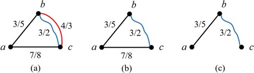
Now, we generalise our above intuitive. Assume that there are two paths p₁ and p₂ between any two nodes on a map, dp₁ and dp₂ denote two travel distances on p₁ and p₂, and tp₁ and tp₂ denote two travel time on p₁ and p₂. If dp₁ ≥ dp₂ and tp₁ ≥ tp₂ exist, then p₁ must not be in any time constrained shortest path. In Figure 1(b), there are two paths p₁: a-c and p₂: a-b-c between a and c. It is easy to verify that the travel distance and time on p₁ are larger than those on p₂. Thus, path p₁ must not be in any time constrained shortest path. Then, we can delete path p₁ in Figure 1(b) and then obtain Figure 1(c).

Our approach is to treat the TCSPP with the above two subjective intuitions as two Lagrangian relaxation techniques. To realise our approach, we use formal method to describe these two subjective intuitions, and design an algorithm to realise our approach in the following sections.

4. Preliminary

Given the weighted graph G = <V, E, W>, where V is the node set, E is the edge set linking any two nodes, and W is the weight set on the edges. Let P = {p_i | 1 ≤ i ≤ n} denote the set of the paths between two nodes in G.

Definition 1

DWG and TTWG

The weighted graph G is called the distance weighted graph (DWG) or the travel time weighted graph (TTWG) if W consists of the distance d (d ∈ W) on the edge or travel time t (t ∈ W) on the edges.

In an actual map, the distance between two nodes is definite, whereas the travel time of the vehicle between two nodes is undefinite. Thus, we respectively construct DWG and TTWG in the following sections so that TTWG can be dynamically adjusted according to the actual situation.

Let D_i=  ∑d be the sum of weighted distances (SWD) on path p_i in DWG and T_i = ∑t be the sum of weighted time (SWT) on path p_i. It is given that (v₁, d, v₂) and (v₁, t, v₂) are two edges that are started with v₁ and ended with v₂ in DWG and TTWG, respectively, and tc denotes a specific time constraint.

Definition 2

the time constrained shortest path

In both DWG and TTWG, there is a path p_k ∈ P from v_i to v_j, in which the SWT is t_k on p_k, the SWD is d_k on p_k, and t_k ≤ tc. Path p_k is called the time constrained shortest path from v_i to v_j if for any p_i ∈ P (I ≠ k) with the travel time t_i on p_i, and the SWD d_i on p_i, there are d_k ≤ d_i and t_i ≤ tc, or d_k > d_i and t_i > tc.

Theorem 1:

Given two edges e₁ = (v₁, d₁, v₂) and e₂ = (v₁, d₂, v₂), and t₁ and t₂ are time weights on e₁ and e₂, respectively. Any time constrained shortest path does not cover edge e₁ when d₁ ≥ d₂ and t₁ ≥ t₂.

Proof: (by contradiction):

Assumption 1. There is a time constrained shortest path p_ij = p_i1 − e₁ − p_2j from v_i to v_j, where p_i1 is the path from v_i to v₁ and p_2j is the path from v₂ to v_j. Let d_i1 be the SWD on p_i1, d_2j the SWD on p_2j, and d_ij the SWD on p_ij. Let t_i1 be the SWT on p_i1, t_2j the SWT on p_2j, and t_ij the SWT on p_ij.

Thus, we get (1) $d_{ij}={d_i}_1+d_1+d_{2j}$(1) and (2) $t_{ij}={t_i}_1+t_1+t_{2j}$(2) Let p′ = p_i1 − e₂ − p_2j be a path from v_i and v_j in the graph, p′ the SWD on p′, and t′ the SWT on p′. Thus, there are (3) $p^{\mathrm{\prime }}={p_i}_1+d_2+p_{2j}$(3) and (4) $t^{\mathrm{\prime }}={t_i}_1+t_2+t_{2j}$(4) Because there are d₁ ≥ d₂ and t₁ ≥ t₂, we can obtain (5) $d_{ij}\ge d^{\mathrm{\prime }}$(5) and (6) $t_{ij}\ge t^{\mathrm{\prime }}.$(6) For time constraint tc, there are three cases: (1) tc < t′ ≤ t_ij, (2) t′ ≤ tc < t_ij, and (3) t′ ≤t_ij ≤ tc.

When tc < t′≤t_ij or t′≤ tc < t_ij, because travel time t_ij on path p_ij does not satisfy time constraint tc, path p_ij is not a time constrained shortest path according to definition 2. When t′ ≤ t_ij ≤ tc, because d_ij ≥ d′ exists in Equation (5), path p_ij is also not a time constrained shortest path according to definition 2. Hence, path p_ij must not be a time constrained shortest path, and the assumption is wrong. The time constrained shortest path then must not contain edge e₁.

Theorem 2:

Assume that p₁ and p₂ are two paths from v_i to v_j in the graph; d₁ and d₂ are two SWTs on p₁ and p₂, respectively; and t₁ and t₂ are two SWTs on p₁ and p₂, respectively. The time constrained shortest path from v_i to v_j must not contain p₁ if d₁ ≥ d₂ and t₁ ≥ t₂.

Theorem 2 is an extension of theorem 1. If we take p₁ and p₂ as two edges from v_i to v_j, theorem 2 can be proved in a similar way to theorem 1. According to theorems 1 and 2, we can simplify the graph to reduce the runtime of our algorithm for solving the TCSPP.

5. Our algorithm

Our algorithm consists of three stages: (1) reduce the graph according to theorems 1 and 2, and then construct the DT graph; (2) transform the DT graph into a variant DT tree with the destination as the root and the source as the leaf, and (3) obtain the time constrained shortest path in the variant DT tree by calculating the minimal difference value. An example, shown in Figure 1, is used to illustrate three stages of our algorithm.

5.1. Construction of DT graph

Definition 3

dt node

In the graph, the distance–time (dt) node of the node v is defined as v(∑d, ∑t), where ∑d denotes the SWD on the path from the source to v, and ∑t denotes the SWT on the path from the source to v.

By Definition 3, a path corresponds to a dt node.

Definition 4

initial dt₀

In the graph, dt₀ = v₀(0, 0) is the initial dt when v₀ is the source.

Definition 5

reducible dt and relevant dt

In the graph, if there are dt₁ = v(∑d₁, ∑t₁) and dt₂ = v(∑d₂, ∑t₂) that satisfy ∑d₁ ≥ ∑d₂ and ∑t₁ ≥ ∑t₂, dt₁ is called the reducible dt. Both dt₁ and dt₂ are called the relevant dt of node v.

Theorem 3:

There is not a time constrained shortest path corresponds to a reducible dt.

Proof

(by contradiction):

Assumption 1: There is a time constrained shortest path p from v₀ to v corresponding to a reducible dt = v(∑d, ∑t).

By Definition 5, there must be a dt₁= v(∑d₁, ∑t₁) from v₀ to v, satisfying ∑d ≥ ∑d₁ and ∑t ≥ ∑t₁. Thus, there must be a path p₁ from v₀ to v corresponding to dt₁. By Definition 3, the length of p₁ is ∑d₁ and the time consumption on p₁ is ∑t₁, while the length of p is ∑d and the time consumption on p is ∑t. Because there are ∑d ≥ ∑d₁ and ∑t ≥ ∑t₁, p is not a time constrained shortest path according to Definition 2, which contradicts Assumption 1. Thus Assumption 1 is wrong and Theorem 3 is proved.

Definition 6

DT graph:

The DT graph is defined as DTG = <M_dt, D/T, dt₀>, where

• M_dt is the set of all dt nodes, where ∑d in the dt node denotes the SWD on the shortest path from the source to v;

• D is the set of the distances on the edges of the DWG, T is the set of the travel time on the edges of the TTWG, and D/T denotes the set of edges;

• dt₀ denotes an initial dt of the DT graph.

Assume that v is directly connected by nodes v₁, v₂, … , v_i. Then, the dt node of v dt = v(∑d, ∑t) yields to (7) $\sum d=MIN(\sum d_1+{d_k}_1,\sum d_2+{d_k}_2,\dots ,\sum d_i+d_{ki}),$(7) where ∑d_j denotes the SWD on the shortest path from the source to v_j, d_kj denotes the distance from v_j to v, and 1 ≤ j ≤ i.

In the DT graph, dt = v(∑d, ∑t) denotes a node and d/t ∈D/T denotes an edge. Given that the array dt[0..n] records all dts, the array Path[0..n] records precursor nodes of a node and distance/time (d/t for short) on the edge, and the set E stores those dts that are connected by dt in the array dt[0..n] and are not reducible dts. Then, we design Algorithm 1 to construct a DT graph from both a DWG and a TTWG.

Table

Algorithm 1 ConstructDTGraph

Input: A DWG and a TTWG;

Output: Two arrays dt[0..n] and Path[0..n];

Initialize dt[0] = v0(0,0), Path[0..n] = {}, E = {}, m = 0, and mark v0 as a visited node;

Get v(∑d, ∑t) from dt[m] and visited nodes v1,· · ·, vk that directly connect v;

for i = 0 to k do

Obtain the edge dj = tj from vi to v;

Get vi(∑di, ∑ti) from the array dt[0..n];

Sd = ∑di + dj and St = ∑ti + tj;

if Sd < ∑d or St < ∑t then

Path[m] = Path[m] ∪ (vi, di = ti);

end if

end for

Get unvisited nodes v1,· · ·, vk that are directly connected by the node v in v(∑d, ∑t);

for i = 0 to k do

Obtain di = ti on the edge from v to vi;

Sd = ∑di + dj and St = ∑ti + tj;

E = E ∪ {vi(Sd, St)};

end for

Delete all reducible dts in E;

Pick up dti with the minimum ∑d from E, and mark vi in dti as a visited node;

dt[+ + m] = dti;

Delete all relevant dts of vi in E;

Repeat step 2 to step 20, until E is an empty set;

return dt and Path;

The main idea of algorithm 1 is to constantly build both the dt node in M_dt and the edge (d/t) between two dt nodes in the DT graph by means of the on-the-fly method to traverse the graph. Also, algorithm 1 does not need input both a specific time constraint and a destination to construct the DT graph. Because algorithm 1 has just visited all edges once in both the DWG and the TTWG, its time complexity is O(e), where e is the total number of edges in the DWG.

Figure 2 (a) and (b) are a DWG and a TTWG, respectively, where all weights are labelled on the edges. The red edges in both the DWG and the TTWG must not be contained in any time constrained shortest path according to theorem 1. Assume that node A is the source. Table 1 shows the implementation of Algorithm 1. Using both dt[0..n] and Path[0..n] in Table 1, we build a DT graph of the DWG and the TTWG in Figure 2(a) and (b), which is shown in Figure 2(c).

Figure 2. An example for illustrating our approach.

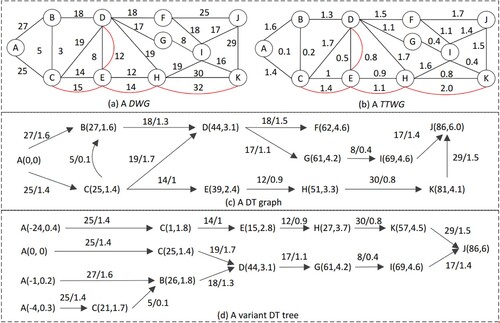
Table 1. The process of constructing the DTG from both the DWG and the TTWG shown in Figure 2 (a) and (b).

Step	dt[0..n]	Path[0..n]	E
1	A(0, 0)	{}	{B(27, 1.6), C(25, 1.4)}
2	C(25, 1.4)	{(A, 25/1.4)}	{B(27, 1.6), B(30, 1.5), D(44, 3.1), E(39, 2.4)}
3	B(27, 1.6)	{(A, 27/1.6), (C, 5/0.1)}	{D(44, 3.1), E(39, 2.4), D(45, 2.9)}
4	E(39, 2.4)	{(C, 14/1)}	{D(44, 3.1), D(45, 2.9), H(51, 3.3)}
5	D(44, 3.1)	{(B, 18/1.3), (C, 19/1.7)}	{H(51, 3.3), F(62, 4.6), G(61, 4.2)}
6	H(51, 3.3)	{(E, 12/0.9)}	{F(62, 4.6), G(61, 4.2), I(70, 4.9), K(81, 4.1)}
7	G(61, 4.2)	{(D, 17/1.1)}	{F(62, 4.6), K(81, 4.1), I(69, 4.6)}
8	F(62, 4.6)	{(D, 18/1.5)}	{K(81, 4.1), I(69, 4.6), J(87, 6.3)}
9	I(69, 4.6)	{(G, 8/0.4)}	{K(81, 4.1), J(86, 6)}
10	K(81, 4.1)	{(H, 30/0.8)}	{J(86, 6), J(110, 5.6)}
11	J(86, 6.0)	{(I, 17/1.4), (K, 29/1.5)}	{}

Note that in Table 1, set E in those steps does not contain reducible dts. For example, in Step 2, because nodes B, D, and E connect C, we can obtain E = {B(27, 1.6), B(30, 1.5), D(44, 3.1), E(39, 2.4), E(40, 2.8)}. However, E(40, 2.8) in set E is a reducible dt node, so it must be deleted from E. Then, we can select a dt node with minimum distance in E as the next element in dt[0..n], such as all the red underlined dt nodes in E in Table 1. Using both dt[0..n] and Path[0..n] in Table 1, we build a DT graph of the DWG and the TTWG in Figure 2(a) and (b), which is shown in Figure 2(c).

Compared with both the DWG and the TTWG, the DT graph is a directed graph starting at the initial dt, and all dt nodes in the DT graph are reached by one or more directed edges except for the initial dt. Because, in the DT graph, the paths that must not be contained in anyone time constrained shortest path are eliminated, the DT graph retains all shortest paths from the source to any other nodes that satisfy any time constraints. The space of the DT graph is less than that of the DWG or the TTWG. The total number of edges in the DT graph shown in Figure 2(c) is 13, whereas that in the DWG or in the TTGW shown in Figure 2(a) and (b) is 48.

5.2. Construction of variant DT tree

To obtain a time constrained shortest path, we need to construct a variant DT tree.

Definition 7

variant dt node

The variant dt node of the node v is defined as vdt = v(Sd, St), where Sd represents the distance, and S_t represents the travel time.

Definition 8

initial variant dt node

The initial variant dt node is a dt node of the destination in the DT graph.

If d₁/t₁ is an edge from v_i(∑d_i, ∑t_i) to v_j(∑d_j, ∑t_j) in the DT graph, both v_i(Sd_i, St_i) and v_j(Sd_j, St_j) satisfy the following formulas: (8) $S{d}_i=S{d}_j-d_1$(8) and (9) $S{t}_i=S{t}_j-t_1$(9)

Definition 9

variant DT tree

The variant DT tree with at least a variant dt is defined by VDT = <M_vdt, D/T, vdt₀>, where

• M_vdt is the set of the variant dt nodes, where for any two variant dt nodes, if one is the child node of the other, they satisfy formulas (8) and (9);

• D/T denotes the set of the edges, and all the edges are pointing in the same direction in the DT graph;

• vdt₀ is the initial variant dt node, which is the dt node of the destination in the DT graph.

Given that Tree[0..n][3] stores the variant dt tree, where Tree[0..n][0] stores the variant dt node, Tree[0..n][1] stores the father node of Tree[0..n][0], and Tree[0..n][2] stores the edge of Tree[0..n][0] to its father node. Let list be a list to store those variant dt nodes. Algorithm 2 for constructing the variant DT tree is then as follows:

Table

Algorithm 2: ConstructVariantDTTree

Input: the array dt[0..n] and the array Path[0..n];

Output: the array Tree[0..n][3] the variant DT tree.

Initialize high = 0 and a list list is empty;

Get the initial variant dt node vdt from dt[0..n]; //This is the destination.

Tree[high][0] = vdt;

Tree[high][1] = −1; // Tree[high][1] = −1 denotes that the node is the root of the variant dt Tree.

Tree[high][2] = 0/0;

List = Tree[high++][0];

while(list is not empty)

Output a vdt from list;

Find its precursor nodes from both dt[0..n] and Path[0..n];

for each precursor node in dt[0..n]

Construct the vdt according to formulas in (8) and (9);

Tree[high][0] = vdt;

Tree[high][1] = n; //n is the position of vdt in list.

Tree[high][1] = d/t; //d/t is the edge coming from Path[0..n].

List = Tree[high++][0];

end for

end while

return Tree;

Assume that the destination is J in the DT graph shown in Figure 2(c). According to algorithm 2, we obtain a variant DT tree that is shown in Figure 2(d). The time constrained shortest path is one of the paths from the leaves to the root in the variant DT.

As shown in Figure 2(d), the variant DT tree consists of the variant dts taken as the nodes and the distance/time taken as the edges. In the variant DT tree, all leaves are the variant dt nodes of the source. When the destination has changed, we only must rebuild a new variant DT tree with the new destination taken as the root without constructing the DT graph again. Therefore, our algorithm can easily generate a time constrained shortest path from one node to other nodes. In addition, algorithm 2 does not need to input the specific time constraint, and the constructed variant DT tree may not contain all nodes in the DT graph. For example, the dt node of node F in the DT graph in Figure 2(c) is not contained in this variant DT tree in Figure 2(d). Thus, the space of the variant DT tree is generally less than that of the DT graph. Because algorithm 2 must access all dt nodes in dt[0..n] and their precursors stored in Path[0..n] once, its time complexity is O(n).

5.3. Calculation of the time constrained shortest path

Given that the root is v(Sd, St) and the leaf is v(Sd_i, St_i) in a variant DT tree, the time constrained shortest path can be obtained by using the following calculations: (11) $\text{min}\left(Sd-S{d}_i\right)$(11) and (12) $\left(St-S{t}_i\right)\le tc$(12)

For example, assume that there are six time constraints tc₁ = 7, tc₂ = 6, tc₃ = 5.8, tc₄ = 5.7, tc₅ = 5.6, and tc₆ = 5.5. Then, according to the formulas (4) and (5), we obtain six shortest paths to respectively satisfy six time constraints from the variant DT tree in Figure 2 (d). Table 2 shows the six time constrained shortest paths, where Null denotes that there is not a shortest path can satisfy the given time constraint, and Distance and Time denote the SWD and the SWT on the time constrained shortest path, respectively.

Table 2. Six time constrained shortest paths.

Time constraint	Path	Distance	Time
tc1 = 7	A(0,0)-C(25,1.4)-D(44,3.1)-G(61,4.2)-I(69,4.6)-J(86,6)	86	6
tc2 = 6	A(0,0)-C(25,1.4)-D(44,3.1)-G(61,4.2)-I(69,4.6)-J(86,6)	86	6
tc3 = 5.8	A(−1,0.2)-B(26,1.8)-D(44,3.1)-G(61,4,2)-I(69,4.6)-J(86,6)	87	5.8
tc4 = 5.7	A(−4,0.3)-C(21,1.7)-B(26,1.8)-D(44,3.1)-G(61,4.2)-J(86,6)	90	5.7
tc5 = 5.6	A(−24,0.4)-C(1,1.8)-E(15,2.8)-H(27,3.7)-K(54,4.5)-I(69,4.6)-J(86,6)	110	5.6
tc6 = 5.5	Null	Null	Null

Note that if all leaves in the variant DT tree do not satisfy formulas (11) and (12), there is not a time constrained shortest path in the graph. If the source node A is replaced by other nodes in this example, we must relaunch algorithms 1 and 2. If the given time constraint is changed, we only need to recalculate in terms of formulas (11) and (12) to obtain the shortest path that satisfies the given time constraint.

6. Experiment

We have conducted an experiment to compare our algorithm with several classical graph algorithms on both the number of algorithms’ iterations and the algorithms’ runtime on a transportation map.

6.1. Experimental settings and environment

The selected algorithms include a FIFO-based algorithm(FIFO), FILO-based algorithm (FILO), Belleman–Ford-based algorithm (BF), Dijkstra-based algorithm (Dijkstra), and our algorithm named the DT algorithm (DTA). The experimental environment is the Windows 10 operating system running on a Lenovo K27, where the CPU is a Core i3 and the memory size is 4 GB. All experimental results have been obtained from the console of Jbuilder 2006. In the experiment, we use the Java statement “System.currentTimeMillis()” to count the running time of each algorithm, and all algorithms have been launched on the Shanghai Chongming Island road map with 78 nodes and 264 edges.¹ To facilitate the implementation of these algorithms, we have set up a unique travel time for each road on the map.

To compare the efficiency of these algorithms, we have randomly selected ten pairs of nodes as both the source and the destination from the map and set up five different travel times. We then launched these algorithms to solve the time constrained shortest path on the map.

6.2. Experimental result

The comparison results of the five algorithms are shown in Figure 3, where Figure 3(a) is the maximal iteration number of five algorithms on ten pairs of nodes as both the sources and the destinations, and Figure 3(b) is the runtime of five algorithms on ten pairs of nodes as both the sources and the destinations.

Figure 3. Experimental results for both the maximal iteration number and the runtime of five algorithms.

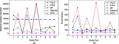
From Figure 3(a), some significant phenomena can be observed. (1) The maximal iteration number of DTA is lowest on all pairs of nodes except the third pair. (2) The maximal iteration number of both DTA and BF is more stable than that of other algorithms. (3) In the third pair of nodes, the maximal iteration number of FILO is less than that of DTA. By looking for the randomly selected pair of nodes, we find that the third pair of nodes is nearby on the map. As a result, FILO can find a time constrained shortest path without traversing too many nodes on the map. (4) The maximal number of iterations for DTA is approximately 600, whereas the maximal number of iterations for the other algorithms is at least 5000.

From Figure 3(b), we can obtain some significant phenomena. (1) In general, the five algorithms’ runtimes correspond with the maximal iteration number in these algorithms shown in Figure 3(a). (2) Compared with the other algorithms, the runtime of DTA is lowest on all except the third and fifth pairs of nodes. A similar reason in the experiment for the maximal iteration number of the algorithm in the third pair of nodes can explain the phenomenon in the third pair of nodes in Figure 3(b). For the fifth pair of nodes, the runtime of Dijkstra is less than that of DTA. By debugging the Dijkstra algorithm, we find that because the first shortest path found by Dijkstra satisfies the given time constraint, backtracking of the whole graph space is unnecessary. In contrast, DTA first must transform the original map into the DT graph, which is equivalent with Dijkstra without backtracking. DTA then constructs a variation DT tree from the DT graph. Finally, DTA can obtain a path that satisfies the time constraint by calculating the difference value between the root and the leaves according to formulas (9) and (10). Therefore, DTA spends more time than Dijkstra to generate the variation DT in the fifth pair of nodes. (3) The runtime of BF is approximately 100, whereas that of our algorithm is 50. Comparing Figure 3(a) with Figure 3(b), the maximal iteration number of BF is approximately 14,000, but its runtime is approximately 100. (4) For the runtime, both DTA and BF are stable, both FIFO and FILO have rapid changes, and Dijkstra is medium.

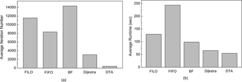
Based on the above experimental result, we count the average iteration number of five algorithms and their average runtime, and the statistical result is shown in Figure 4. From Figure 4(a), the average iteration number of DTA is approximately 500, that of Dijkstra is approximately 3000, that of FIFO is approximately 8000, that of FILO is approximately 11,000, and that of BF is more than 14,000. Therefore, the average iteration number of DTA is far better than those of the other algorithms. From Figure 4(b), the average runtime of DTA is also better than those of the other algorithms. In addition, a surprising phenomenon is that the average runtime of BF is better than those of FILO and FIFO, but it has more average iterations in the experiment as shown in Figure 4(a).

Figure 4. Experimental results for both the average iteration number and the average runtime of five algorithms.

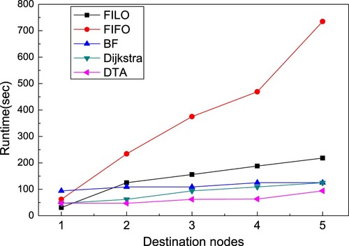
One of the advantages of DTA is that it can be launched to construct the DT graph without obtaining both the destination and the specific time constraint. Thus, we have conducted an experiment to observe the runtime of five algorithms for solving the shortest paths from a source to several different destinations, satisfying a given time constraint. Figure 5 shows the experimental result. From Figure 5, with increasing number of the destinations, the runtime of all algorithms also increases. DTA always has the minimal runtime when the number of the destinations is greater than 1. In addition, the growth rate of the runtime of both DTA and BF is slower than the other algorithms.

Figure 5. The experimental comparison of five algorithms with 5 destinations.

We then conducted an experiment to compare the runtime on five algorithms for solving the shortest path with four time constraints (including 200, 240, 250, and 300 ms). Figure 6 shows this experimental result.

Figure 6. The experimental comparison of five algorithms with four different time constraints.

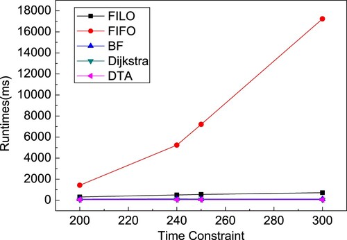
From Figure 6, we find that with increasing number of time constraints, the runtime of FIFO shows an exponential growth, whereas the runtime of FILO indicates linear growth, and the runtimes of the other algorithms imply a slow increase.

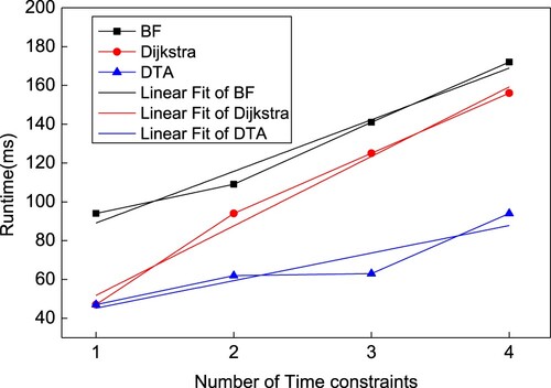
To compare the linear growth rate of BF, Dijkstra, and DTA, we linearly fit three algorithms BF, Dijkstra, and DTA. We set a source node and a destination and then add four different time constraints in the process of solving the time constrained shortest paths. The fitting result is shown in Figure 7. From Figure 7, with increasing number of time constraints, the runtimes of the three algorithms also increase. The runtime of our algorithm (DTA) is lower than those of BF and Dijkstra in the experiment. In addition, we find that the growth rate of time consumption for DTA is less than those of BF and Dijkstra. Therefore, DTA has higher time efficiency for solving the shortest path that satisfies the changing time constraints.

Figure 7. Experiment for the incremental time constraints.

6.3. Experimental conclusions

To sum up, the runtime of DTA (our algorithm) is relatively stable when both the destination and the time constraint are changed. With increasing number of both destinations and time constraints, the runtime of DTA grows slowly. Thus, for the TCSPP from one node to some destinations, our algorithm is a better selection than the existing graph algorithms in our experiments. In addition, DTA has the lowest average iteration number and the average runtime. In most cases, the efficiency of DTA is better than that of classical graph algorithms.

7. Conclusion and future work

We have presented a novel graph algorithm to solve the TCSPP. Our algorithm contains three stages: (1) transform the undirected graph into a directed DTG based on two proposed theorems, (2) construct a variant DT tree with the destination taken as the root and the source regarded as the leaves, and (3) calculate a time constrained shortest path by comparing the leaves on the variant DT tree. The core idea of our algorithm is to employ two new Lagrangian relaxation techniques to eliminate the edges and reduce the graphic space. In contrast to some existing algorithms, our algorithm can be launched without entering either the specific time constraint or the destination. At the same time, it can quickly find a shortest path when the destination and travel time are changed on the map. Therefore, our algorithm is more suitable for looking for the shortest path from one source to multiple destinations as well as with varying travel time. In the future, we plan to extend our algorithm for solving the multi-constraint shortest path problem.

Author contribution

Conceptualization Ideas: Pan Liu and Wulan Huang; Methodology: Pan Liu and Wulan Huang; Software: Pan Liu; Validation: Pan Liu and Wulan Huang; Formal Analysis: Pan Liu and Wulan Huang; Investigation: Pan Liu; Writing – Original Draft: Pan Liu and Wulan Huang; Writing – Review & Editing: Wulan Huang and Pan Liu; Supervision: Pan Liu.

Acknowledgments

The authors would like to thank the anonymous reviewers for their constructive and insightful comments on this paper.

Disclosure statement

No potential conflict of interest was reported by the author(s).

Additional information

Funding

This work was supported in part by National Social Science Fund General Project of China under [grant number 18BTQ058] and the Science and Technology Key Project of Jiangxi Province under [grant number 20142BBE50015].

Notes

1 A Java class of our algorithm is developed for this experiment and the download link with the password PAN1 is https://pan.baidu.com/s/1kFlM4g4XZnzgwJVD1Uc9pw.

References

- Akram, M., Habib, A., & Alcantud, J. C. R. (2021). An optimization study based on Dijkstra algorithm for a network with trapezoidal picture fuzzy numbers. Neural Computing and Applications, 33(4), 1329–1342. https://doi.org/10.1007/s00521-020-05034-y
- Aneja, Y. P., Aggarwal, V., & Nair, K. P. (1983). Shortest chain subject to side constraints. Networks, 13(2), 295–302. https://doi.org/10.1002/net.3230130212
- Barbehenn, M. (1998). A note on the complexity of Dijkstra's algorithm for graphs with weighted vertices. IEEE Transactions on Computers, 47(2), 263. https://doi.org/10.1109/12.663776
- Barrett, C., Bisset, K., Jacob, R., Konjevod, G., & Marathe, M. (2002). Classical and contemporary shortest path problems in road networks: Implementation and experimental analysis of the TRANSIMS router. Paper presented at the European Symposium on Algorithms, Rome, Italy, 17-21 Sept. 2002. https://doi.org/10.1007/3-540-45749-6_15
- Beamer, S., Asanović, K., & Patterson, D. (2013). Direction-optimizing breadth-first search. Scientific Programming, 21(3-4), 137–148. https://doi.org/10.1109/SC.2012.50
- Beasley, J. E., & Christofides, N. (1989). An algorithm for the resource constrained shortest path problem. Networks, 19(4), 379–394. https://doi.org/10.1002/net.3230190402
- Broumi, S., Bakal, A., Talea, M., Smarandache, F., & Vladareanu, L. (2016). Applying Dijkstra algorithm for solving neutrosophic shortest path problem. Paper presented at the 2016 International conference on advanced mechatronic systems (ICAMechS), Melbourne, VIC, Australia, 30 Nov.-3 Dec. 2016. https://doi.org/10.1109/ICAMechS.2016.7813483
- Cai, X., Kloks, T., & Wong, C. (1996). Shortest path problems with time constraints. Paper presented at the International Symposium on Mathematical Foundations of Computer Science, Lecture Notes in Computer Science, vol 1113. Springer, Berlin, Heidelberg, 1996. https://doi.org/10.1007/3-540-61550-4_153
- Carlyle, W. M., Royset, J. O., & Kevin Wood, R. (2008). Lagrangian relaxation and enumeration for solving constrained shortest-path problems. Networks: An International Journal, 52(4), 256–270. https://doi.org/10.1002/net.20247
- Chabini, I., & Lan, S. (2002). Adaptations of the A* algorithm for the computation of fastest paths in deterministic discrete-time dynamic networks. IEEE Transactions on Intelligent Transportation Systems, 3(1), 60–74. https://doi.org/10.1109/6979.994796
- Chen, S., & Nahrstedt, K. (1998). On finding multi-constrained paths. Paper presented at the ICC'98. 1998 IEEE International Conference on Communications. Conference Record. Affiliated with SUPERCOMM'98 (Cat. No. 98CH36220), Atlanta, GA, USA, 7-11 June, 1998. https://doi.org/10.1109/ICC.1998.685137
- Chen, S., Song, M., & Sahni, S. (2008). Two techniques for fast computation of constrained shortest paths. Networking, IEEE/ACM Transactions on, 16(1), 105–115. https://doi.org/10.1109/TNET.2007.897965
- Chiu, Y.-H., Lin, Y.-K., & Nguyen, T.-P. (2021). Network reliability of a stochastic online-food delivery system with space and time constraints. International Journal of Performability Engineering, 17(5), 433. https://doi.org/10.23940/ijpe.21.05.p3.433443
- Desrochers, M., & Laporte, G. (1991). Improvements and extensions to the Miller-Tucker-Zemlin subtour elimination constraints. Operations Research Letters, 10(1), 27–36. https://doi.org/10.1016/0167-6377(91)90083-2
- Desrosiers, J., Dumas, Y., Solomon, M. M., & Soumis, F. (1995). Time constrained routing and scheduling. Handbooks in Operations Research and Management Science, 8, 35–139. https://doi.org/10.1016/S0927-0507(05)80106-9
- Dumitrescu, I., & Boland, N. (2003). Improved preprocessing, labeling and scaling algorithms for the weight-constrained shortest path problem. Networks: An International Journal, 42(3), 135–153. https://doi.org/10.1002/net.10090
- Guerrero Roman, I., & Perez y Perez, R. (2020). A methodology to forecast some attributes of an automatic storyteller’s outputs. Connection Science, 32(1), 81–111. https://doi.org/10.1080/09540091.2019.1609418
- Guerriero, F., Di Puglia Pugliese, L., & Macrina, G. (2019). A rollout algorithm for the resource constrained elementary shortest path problem. Optimization Methods and Software, 34(5), 1056–1074. https://doi.org/10.1080/10556788.2018.1551391
- Hohzaki, R., Fujii, S., & Sandoh, H. (1996). A shortest path problem on the network with AGV-type time-windows. Journal of the Operations Research Society of Japan-Keiei Kagaku, 39(1), 77–87. https://doi.org/10.15807/jorsj.39.77
- Irnich, S., & Desaulniers, G. (2005). Shortest path problems with resource constraints. Springer. https://doi.org/10.1007/0-387-25486-2_2
- Jepsen, M. K., Petersen, B., Spoorendonk, S., & Pisinger, D. (2014). A branch-and-cut algorithm for the capacitated profitable tour problem. Discrete Optimization, 14, 78–96. https://doi.org/10.1016/j.disopt.2014.08.001
- Jiang, J.-R., Huang, H.-W., Liao, J.-H., & Chen, S.-Y. (2014). Extending Dijkstra's shortest path algorithm for software defined networking. Paper presented at the The 16th Asia-Pacific Network Operations and Management Symposium, Hsinchu, Taiwan, 17-19 Sept. 2014. https://doi.org/10.1109/APNOMS.2014.6996609
- Joyner, D., Van Nguyen, M., & Cohen, N. (2010). Algorithmic graph theory. Google Code. https://google-code-archive-downloads.storage.googleapis.com/v2/code.google.com/graphbook/latest-r1984.pdf
- Kjerrstrom, J. (2001). The resource constrained shortest path problem. resource, 1. http://citeseerx.ist.psu.edu/viewdoc/download?doi=10.1.1.101.7348&rep=rep1&type=pdf
- Kot, M. (2003). The state explosion problem. Retrieved May, 18, 2015. http://www.cs.vsb.cz/kot/download/Texts/StateSpace.pdf
- Lamatsch, A. (1992). An approach to vehicle scheduling with depot capacity constraints. In M. Desrochers & J. M. Rousseau (Eds.), Computer-aided transit scheduling. Lecture notes in economics and mathematical systems (Vol. 386, pp. 181–195). Springer. https://doi.org/10.1007/978-3-642-85968-7_13
- Li, Y., He, R., Zhang, Z., & Guo, Y. (2005). Models and algorithms for shortest paths in a time dependent network. Paper presented at the International Symposium on OR and its Applications (pp. 319-328).
- Liao, X., Wang, J., & Ma, L. (2021). An algorithmic approach for finding the fuzzy constrained shortest paths in a fuzzy graph. Complex & Intelligent Systems, 7(1), 17–27. https://doi.org/10.1007/s40747-020-00143-6
- Liu, P., Kou, M. H., Ping, Y. G., & Liang, Y. (2008). A new practical algorithm for the shortest path problem. Paper presented at the 2008 7th World Congress on Intelligent Control and Automation, Chongqing, China, 25-27 June, 2008. https://doi.org/10.1109/WCICA.2008.4594514
- Lu, C.-C., Liu, J., Qu, Y., Peeta, S., Rouphail, N. M., & Zhou, X. (2016). Eco-system optimal time-dependent flow assignment in a congested network. Transportation Research Part B: Methodological, 94, 217–239. https://doi.org/10.1016/j.trb.2016.09.015
- Mehlhorn, K., & Ziegelmann, M. (2000). Resource constrained shortest paths. Paper presented at the European Symposium on Algorithms (pp. 326-337), vol 1879. Springer, Berlin, Heidelberg. https://doi.org/10.1007/3-540-45253-2_30
- Mesquita, M., & Paixão, J. (1992). Multiple depot vehicle scheduling problem: A new heuristic based on quasi-assignment algorithms. In M. Desrochers & J. M. Rousseau (Eds.), Computer-aided transit scheduling. Lecture notes in economics and mathematical systems (Vol. 386, pp. 167–180). Springer. https://doi.org/10.1007/978-3-642-85968-7_12
- Mhamedi, T., Andersson, H., Cherkesly, M., & Desaulniers, G. (2022). A branch-price-and-cut algorithm for the two-echelon vehicle routing problem with time windows. Transportation Science, 56(1), 245–264. https://doi.org/10.1287/trsc.2021.1092
- Pugliese, L. D. P., & Guerriero, F. (2013). A survey of resource constrained shortest path problems: Exact solution approaches. Networks, 62(3), 183–200. https://doi.org/10.1002/net.21511
- Righini, G., & Salani, M. (2006). Symmetry helps: Bounded bi-directional dynamic programming for the elementary shortest path problem with resource constraints. Discrete Optimization, 3(3), 255–273. https://doi.org/10.1016/j.disopt.2006.05.007
- Righini, G., & Salani, M. (2008). New dynamic programming algorithms for the resource constrained elementary shortest path problem. Networks: An International Journal, 51(3), 155–170. https://doi.org/10.1002/net.20212
- Tang, J., Song, Y., Miller, H. J., & Zhou, X. (2016). Estimating the most likely space–time paths, dwell times and path uncertainties from vehicle trajectory data: A time geographic method. Transportation Research Part C: Emerging Technologies, 66, 176–194. https://doi.org/10.1016/j.trc.2015.08.014
- Thomas, B. W., Calogiuri, T., & Hewitt, M. (2019). An exact bidirectional A★ approach for solving resource-constrained shortest path problems. Networks, 73(2), 187–205. https://doi.org/10.1002/net.21856
- Wang, S.-H., Tu, C.-H., & Juang, J.-C. (2022). Automatic traffic modelling for creating digital twins to facilitate autonomous vehicle development. Connection Science, 34(1), 1018–1037. https://doi.org/10.1080/09540091.2021.1997914
- Wen, L., Çatay, B., & Eglese, R. (2014). Finding a minimum cost path between a pair of nodes in a time-varying road network with a congestion charge. European Journal of Operational Research, 236(3), 915–923. https://doi.org/10.1016/j.ejor.2013.10.044
- Wu, L., Wei, X., Meng, L., Zhao, S., & Wang, H. (2022). Privacy-preserving location-based traffic density monitoring. Connection Science, 34(1), 874–894. https://doi.org/10.1080/09540091.2021.1993137
- Xia, Z., Wang, X., Sun, X., & Wang, Q. (2016). A secure and dynamic multi-keyword ranked search scheme over encrypted cloud data. IEEE Transactions on Parallel and Distributed Systems, 27(2), 340–352. https://doi.org/10.1109/TPDS.2015.2401003
- Xie, Y.-x., Ji, L.-x., Li, L.-s., Guo, Z., & Baker, T. (2021). An adaptive defense mechanism to prevent advanced persistent threats. Connection Science, 33(2), 359–379. https://doi.org/10.1080/09540091.2020.1832960
- Yang, Y., Gao, H., Yu, J. X., & Li, J. (2014). Finding the cost-optimal path with time constraint over time-dependent graphs. Proceedings of the VLDB Endowment, 7(9), 673–684. https://doi.org/10.14778/2732939.2732941
- Zhang, L., & Xu, J. (2022). Blockchain-based anonymous authentication for traffic reporting in VANETs. Connection Science, 34(1), 1038–1065. https://doi.org/10.1080/09540091.2022.2026888
- Zheng, Z., Zhou, Y., Sun, Y., Wang, Z., Liu, B., & Li, K. (2022). Applications of federated learning in smart cities: Recent advances, taxonomy, and open challenges. Connection Science, 34(1), 1–28. https://doi.org/10.1080/09540091.2021.1936455
- Zhu, X., & Wilhelm, W. E. (2012). A three-stage approach for the resource-constrained shortest path as a sub-problem in column generation. Computers & Operations Research, 39(2), 164–178. https://doi.org/10.1016/j.cor.2011.03.008