
 ?Mathematical formulae have been encoded as MathML and are displayed in this HTML version using MathJax in order to improve their display. Uncheck the box to turn MathJax off. This feature requires Javascript. Click on a formula to zoom.
Abstract
The classification performance of a k-nearest neighbour (KNN) method is dependent on the choice of the k neighbours of a query. However, it is difficult to optimise the performance of KNN by choosing appropriate neighbours and an appropriate value of k. Moreover, the performance of KNN suffers from the use of a simple majority voting method. To address these three issues, we propose a new locally adaptive k-nearest centroid neighbour classification based on the average distance (AD-LAKNCN) in this paper. First, the k neighbours of the query based on the nearest centroid neighbour (NCN) are found, and the discrimination classes with different k values are derived from the number and distribution of each class of neighbours considered in the query. Then, based on the distribution information in the discrimination class for each k, the adaptive k and the final classification result are obtained. The experimental results based on 24 real-world datasets show that the new method achieves better classification performance than nine other state-of-the-art KNN algorithms.
1. Introduction
Classification is the core of pattern recognition, machine learning and data mining. Its essence is to determine which predefined target class to which an object belongs. Considerable attention has been focused on this field, and we have widely applied it in emotion classification (Wang et al., Citation2021; Wei et al., Citation2022; Zhang et al., Citation2022) and food nutrition matching (Zhu et al., Citation2020). At present, the main classification methods include support vector machines (SVMs), decision trees, Bayesian classification, k-nearest neighbour (KNN) classification, and neural networks. Among these methods, the KNN classification algorithm (Cover & Hart, Citation1967) is a simple, effective and nonparametric method. It is also considered one of the top ten algorithms in data mining (Wu et al., Citation2008). Additionally, in the Bayesian sense, it has been proven that under the constraint of , its performance increases gradually with an increasing number of samples
(Guo & Dyer, Citation2005).
While the KNN algorithm has many advantages, it still has some unavoidable problems. First, on small-scale datasets, sparse distribution, imbalance and noise problems (Wen et al., Citation2012) seriously affect the classification performance. Second, the classification effect is sensitive to the choice of . If
is too small, the classification result is susceptible to noise points. If
is too large, there may be more samples with other classes in the neighbourhood, which may cause classification errors for the query point, especially for datasets with unbalanced samples (Gou et al., Citation2012). Third, when the
neighbours of the query point are selected, only the distance is considered, and the distribution near the query point is not considered. Additionally, the majority voting method is generally used in neighbourhood classification; that is, the class of the query point is determined by the class of the majority of the
neighbours. This decision mechanism is simple and rough and does not take into account the distribution of the remaining classes of the
neighbours of the query point. To address the above problems, researchers have proposed many improved KNN-based methods. Next, some of the most advanced KNN-based algorithms are briefly introduced.
Because the KNN algorithm does not consider the weight of each neighbouring point, Dudani developed a weighted voting method called the distance-weighted KNN (WKNN) algorithm (Dudani, Citation1976). The basic idea is to give more weight to samples closer to the query point. Subsequently, Rastin et al. developed a k-nearest neighbour stacking method that uses a feature-weighted distance measure to reduce the effect of irrelevant classes in stacking (Rastin et al., Citation2021). Both of the above methods consider the weight of each neighbouring point, but the reality of choosing weights is that it is insufficient to only consider the distance information.
To solve the problem of the sensitivity of the KNN algorithm to noise points, Mitani et al. presented a local mean KNN (LMKNN) algorithm (Mitani & Hamamoto, Citation2006); this algorithm uses the local mean vector of neighbours from each class to determine the query point class. However, LMKNN does not consider the weight of each neighbouring point. On this basis, Zeng et al. considered the weighted sum of the distances of the neighbours in each class and presented a pseudonearest neighbour (PNN) rule (Zeng et al., Citation2009). Gou et al. extended the PNN algorithm and presented a local mean-based pseudonearest neighbour (LMPNN) algorithm (Gou et al., Citation2014); this algorithm eliminates the influence of outliers by using the
local mean vectors of the neighbours in each class instead of themselves. Moreover, Gou et al. presented a local mean representation-based k-nearest neighbour algorithm (LMRKNN), which uses the multi-local mean vectors of the class-specific
nearest neighbours to linearly represent the testing sample (Citation2019). The above methods mainly use the local mean vectors to eliminate the influence of outliers and achieve satisfactory classification performance. However, the above methods are still sensitive to the selection of the
value.
To address the sensitivity of the KNN algorithm to the choice of , researchers have proposed different schemes to adaptively choose the appropriate
. Mullick et al. used the density and distribution information of the query point's neighbours and used neural networks to learn an appropriate
(Mullick et al., Citation2018). Gou et al. proposed a generalised mean distance-based k-nearest neighbour classifier (GMDKNN) by introducing multiple generalised mean distances and the nested generalised mean distance (Gou et al., Citation2019). Moreover, a locally adaptive KNN based on discrimination classes (DC-LAKNN) was also proposed that can not only choose
adaptively but also consider the role of the second-most-common class of neighbours in the classification process (Pan et al., Citation2020). In order to obtain more convincing and reliable local mean vectors, a globally adaptive k-nearest neighbour classifier based on local mean optimisation was developed (Pan et al., Citation2021). The above methods choose the
value adaptively through different schemes and improve the classification performance of the KNN-based algorithm.
To address unreliability in the selection of the neighbour points, Chaudhuri presented the nearest centroid neighbour (NCN) method (Chaudhuri, Citation1996), which focuses on the neighbourhood of the query point and employs the ideas of distance and symmetry criteria. Based on the NCN, Sanchez et al. proposed a k-nearest centroid neighbour (KNCN) classification algorithm (Śanchez et al., Citation1997), which ensures the accuracy of classification and has been proven to be valid in many fields (Śanchez & Marqúes, Citation2006). To combine the robustness of LMKNN and the validity of KNCN, local mean-based k-nearest centroid neighbour (LMKNCN) was proposed, which uses the local average vectors of the neighbours of each class to determine the class of the query point (Gou et al., Citation2012). Furthermore, Ma et al. used the ideas of PNN and LMKNCN to propose the pseudo nearest centroid neighbour (PNCN) method, which not only considers the local mean vector of the NCN but also incorporates the weighted sum of the distances of the neighbours in each class (Ma et al., Citation2018). Moreover, Gou et al. proposed a representation coefficient-based k-nearest centroid neighbour (RCKNCN) method, which is able to capture both the proximity and the geometry of the k-nearest neighbours and learns to differentiate the contributions of the neighbours to the classification of a testing sample through a linear representation method (Gou et al., Citation2022). These KNN-based methods above mainly use the NCN to select the neighbour points and achieve excellent classification performance.
To further overcome the sensitivity to and improve the KNN-based classification performance, we present a new method for locally adaptive k-nearest centroid neighbour classification based on the average distance (AD-LAKNCN). First,
neighbours of the query based on the NCN are found, and the discrimination classes with different
are derived from the number and distribution of each class of the query's neighbours. Then, based on the distribution information in the discrimination class for each
, the adaptive
and the final classification result are obtained.
The main contributions of this paper are as follows:
The NCN method is applied to query point neighbour selection. The advantage of this method is that when selecting the query point's neighbours, the principle of neighbours and symmetry is followed so that the query point is surrounded by the selected neighbours.
In AD-LAKNCN, the average distance based on multilocal mean vectors is used to select the discrimination class of the query point. The advantage is that when selecting a query point discrimination class, our method not only makes the number of discrimination class samples as large as possible but also makes the centroid of the discrimination class as close as possible to the query point.
We propose a new adaptive
value choice method. The choice of the
The rest of this article is organised as follows. In section 2, we discuss the related methods. In section 3, we introduce the AD-LAKNCN algorithm in detail. To verify our proposed AD-LAKNCN algorithm, a large number of comparative experiments with nine other state-of-the-art KNN-based algorithms are presented in section 4, and the parameters and complexity are discussed. Finally, the conclusions are given in section 5.
2. Related work
In this section, we briefly discuss two related KNN-based classifiers. They are the KNCN and the DC-LAKNN.
For convenience of representation, the following notations are specified: Let denote a training set with
instances from
classes,
be a training sample in
-dimensional space,
be the corresponding class label of
and the
classes be represented as
.
2.1. KNCN
To address the unreliability in the selection of the neighbour points in KNN, Sanchez et al. proposed a KNCN classification algorithm (Śanchez et al., Citation1997). Its classification process considers the distance on the one hand and the distribution of the query point's neighbours on the other hand, which ensures the accuracy of classification. The KNCN predicts its class label as follows:
Find the nearest neighbour of
Find the
For to
do
EndFor
where is the Euclidean distance and
represents the remaining training samples yet to be chosen.
The majority voting rule is used to assign the query
where is the class label of
and
is the Kronecker delta function.
Based on the rationale of the KNCN, it has proven to be an excellent classifier (Śanchez & Marqúes, Citation2006). However, directly taking the majority class as the classification decision result based on the majority voting rule is arbitrary. Moreover, the KNCN is still sensitive to the selection of the value.
2.2. DC-LAKNN
In the classification process of the KNN algorithm, only majority class neighbours in the neighbourhood are used, regardless of the role of all other remaining nearest neighbours. Additionally, KNN are sensitive to the selection of
. To address the above two issues, DC-LAKNN presents a new
value selection method and considers the role of the second-most common class of neighbours in the classification process (Pan et al., Citation2020). Given a query
, DC-LAKNN works as follows:
Stage 1: Selection of the discrimination class.
Use Euclidean distance metrics to choose the
Find the majority classes
Based on multiple local mean vectors, compute the centroids in the majority classes and secondary majority classes
Select the discrimination class
Record the centroid of nearest neighbours
Stage 2: Selection of the adaptive value and classification procedure.
Calculate the distance
Calculate the average rank of each
Based on the rationale of DC-LAKNN, considering the role of the second-most common class of neighbours based on the KNN and using the adaptive value selection method can achieve satisfactory classification performance. However, DC-LAKNN still has the following issues:
The nearest neighbour selection method based on the KNN method is unreliable because it considers only the distance and does not consider the distribution near the query point.
In the classification process, only the majority classes and secondary majority classes are considered, which is incomplete.
In the adaptive
3. The proposed method
In section 3.1, we introduce the motivation for the AD-LAKNCN. In section 3.2, we describe the AD-LAKNCN algorithm in detail. In section 3.3, we present the pseudocode of the AD-LAKNCN algorithm. In section 3.4, we analyze the differences between the proposed AD-LAKNCN and the related methods.
3.1. Motivation
While the KNN algorithm has many benefits, it still has some issues. In the remainder of this section, we will elaborate on three issues and introduce our motivation.
Issue 1: The nearest neighbour selection method based on the nearest neighbourhood criterion is unreliable
In KNN-based methods, the nearest neighbourhood (NN) criterion is the only criterion for selecting neighbours. In contrast, the NCN criterion focuses on the distribution of the query point and employs the concepts of distance and symmetry criteria (Chaudhuri, Citation1996). Moreover, the NCN method has been proven to be effective in multiple KNN-based algorithms (Gou et al., Citation2012; Gou et al., Citation2022; Ma et al., Citation2018; Śanchez et al., Citation1997).
As an example, in Figure , the point set contained in the blue circle represents the set of neighbours of the query point obtained by the NN method, and the point set contained in the black circle represents the set of neighbours of the query point obtained by the NCN method. Although the blue circle contains the nearest neighbourhood set, the neighbour set obtained by the NCN method not only is near the query point but also surrounds the query point, which is more reasonable.
Figure 1. Three examples of the NN and NCN.
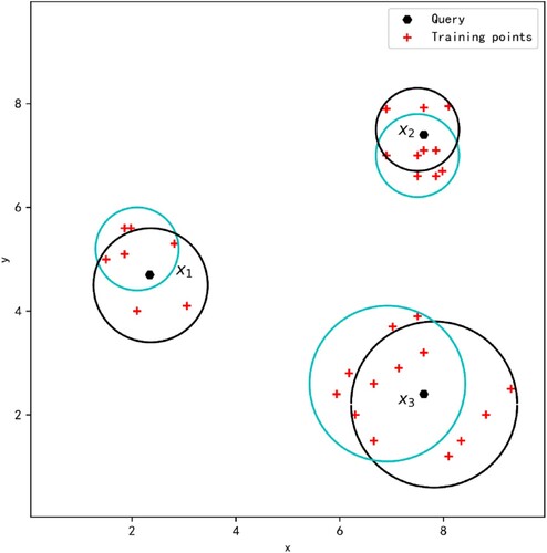
Therefore, we use the NCN method to select the nearest neighbour to improve the classification performance.
Issue 2: It is arbitrary to consider only the majority class
In the classification process of KNN, the majority class of the neighbours of the query is used directly as the result of the classification decision. That is, the classification process does not consider other classes of the neighbours of the query. For this reason, DC-LAKNN uses the information of the majority classes and the secondary majority classes to select the discrimination class, and it obtains satisfactory classification performance.
Inspired by the classification process of DC-LAKNN, we use the average distance between the query and the centroids of all classes of its neighbours to determine the discrimination class. This is advantageous for selecting a query point discrimination class because our method not only makes the number of discrimination class samples as large as possible but also makes the centroid of the discrimination class as close as possible to the query point.
Issue 3: The classification effect is sensitive to the choice of
It is difficult to select an appropriate in KNN. If
is too small, the classification result is susceptible to noise points. If
is too large, there may be more samples with other classes in the neighbourhood, which may cause classification errors for the query point, especially for datasets with unbalanced samples. To address this problem, DC-LAKNN uses the ratio of the number of nearest neighbours in the discrimination class to the number of all nearest neighbours and the distances between the centroids of the nearest neighbours in the discrimination class and the query to adaptively select
. However, it is arbitrary to directly use the mean of the ratio rank and the distance rank to determine the final
. Thus, we redesign the
value selection method to improve the classification performance.
As a result, the main noteworthy characteristics of the proposed AD-LAKNCN are derived from the NCN method, the new discrimination class selection method and the new value selection method. In the next section, the AD-LAKNCN algorithm is described in detail.
3.2. The proposed AD-LAKNCN
In AD-LAKNCN, the classification process consists of two stages. Stage 1 selects the discrimination class of the query point under each value, and stage 2 adaptively selects the best
value. Here, we describe the details of these two stages.
Stage 1: For to
, the best centroid
for each
is found as follows:
According to the NCN method, find
Collate the point set
Calculate the centroid
For
Find the best centroid
First, neighbours of the query point are found iteratively according to the NCN method. Then, the number of samples and the centroid for each class among
neighbours of the query point are calculated. Finally, the discrimination class of the query point is selected based on the average distance. Figure shows three examples.
Figure 2. Examples of the selection of the discrimination class for ,
, and
.
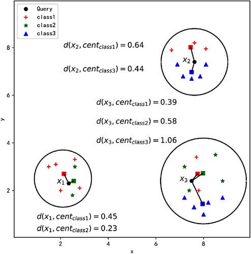
For the query point , the distance from
to the centroid of class 1 is 0.45, and the number of points of class 1 is 5. Therefore, the average distance from
to the centroid of class 1 is
. Similarly, the average distance from
to the centroid of class 2 is
; therefore,
is classified as class 1. For the query point
, the distance from
to the centroid of class 1 is 0.64, and the number of points of class 1 is 3. Therefore, the average distance from
to the centroid of class 1 is
. Similarly, the average distance from
to the centroid of class 3 is
; therefore,
is classified as class 3. For the query point
, the distance from
to the centroid of class 1 is 0.39, and the number of points of class 1 is 2. Therefore, the average distance from
to the centroid of class 1 is
. Similarly, the average distance from
to class 2 is
, and the average distance from
to class 3 is
; therefore,
is classified as class 2.
Stage 2: Find the adaptive for
and its corresponding class
.
Calculate the distance
Calculate the generalised mean distance
We first calculate the distance between the query point and the centroid for the discrimination class and the ratio of the number of nearest neighbours in the discrimination class to the number of all nearest neighbours of each . Then, the final classification result is obtained according to the generalised mean distance.
Both DC-LAKNN and AD-LAKNCN use the distance between the query point and the centroid of the discrimination class and the ratio of the number of nearest neighbours in the discrimination class to the number of all nearest neighbours to adaptively select , which does not exist in KNCN. However, unlike DC-LAKNN, which arbitrarily sorts the ratio and the distance, our method uses the generalised average distance to evaluate the ratio and the distance, which can better capture the local feature distribution of the discrimination class. Figure shows three examples.
Figure 3. Examples of the selection of the adaptive for
,
, and
.
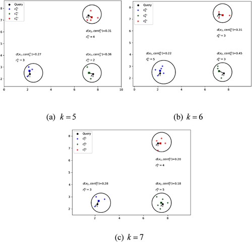
We take and
. For the query point
, the distance from
to the centroid of
is 0.27, and the number of points of
is 3 when
. Therefore, the generalised average distance from
to the centroid of
is
. Similarly, the generalised average distance from
to the centroid of
is 0.05 when
, and the generalised average distance from
to the centroid of
is 0.10 when
. Therefore,
is classified as
. For the query point
, the distance from
to the centroid of
is 0.36, and the number of points of
is 2 when
. Therefore, the generalised average distance from
to the centroid of
is
. Similarly, the generalised average distance from
to the centroid of
is 0.25 when
, and the generalised average distance from
to the centroid of
is 0.10 when
. Therefore,
is classified as
. For the query point
, the distance from
to the centroid of
is 0.31, and the number of points of
is 4 when
. Therefore, the generalised average distance from
to the centroid of
is
. Similarly, the generalised average distance from
to the centroid of
is 0.12 when
, and the generalised average distance from
to the centroid of
is 0.05 when
. Therefore,
is classified as
.
3.3. The algorithm
In this section, we describe the AD-LAKNCN algorithm in detail. The pseudocode for the AD-LAKNCN algorithm is shown in Algorithm 1.
Table
In Algorithm 1, the nearest centroid neighbours of the query point in the training set are computed in steps 1-2, which is the same as KNCN and does not exist in DC-LAKNN. In step 3, the proposed method uses the average distance method to select the discrimination class, which follows both the distance criterion and the quantity criterion. Finally, steps 4 and 5 adaptively select the
value and its corresponding discrimination class as the final class of the query point. Unlike DC-LAKNN, which is arbitrary since it directly uses the mean of the ratio rank and the distance rank to determine the final
, our method uses the generalised average distance to use the ratio and the distance, which can better capture the local feature distribution of the discrimination class. The time complexity of this algorithm is
, where
,
, and
denote the number of training sets, dimensions, and maximum
, respectively.
3.4. Differences between AD-LAKNN, KNCN and DC-LAKNN
In this section, we further analyze the differences between the proposed AD-LAKNCN and related methods, including KNCN and DC-LAKNN.
Both the KNCN and AD-LAKNCN use the NCN method to select the neighbour points. The advantage of this method is that when selecting the query point's neighbours, the principle of neighbours and symmetry is followed so that the query point is surrounded by the selected neighbours. However, in the KNCN, only the majority class is considered, and the sensitivity to the value degrades the classification performance. In the proposed AD-LAKNCN, the average distance between the query and the centroid of each class of the
neighbours is used to determine the discrimination class, and a new adaptive
value selection method is proposed to select the best
value and is employed for good classification.
In DC-LAKNN, the quantity and distribution information of both majority class neighbours and secondary majority class neighbours are considered, and a adaptive value selection method is proposed. Unlike DC-LAKNN, AD-LAKNCN uses the NCN method to select the neighbour points and improves the adaptive
value selection method. Moreover, AD-LAKNCN uses the average distance between the query and the centroid of each class of the
neighbours to determine the discrimination class. In contrast to DC-LAKNN, the proposed AD-LAKNCN not only uses a more reliable nearest neighbour selection method but also incorporates the information of all
nearest neighbours to fully use their distribution information.
4. Experiments
In this section, AD-LAKNCN is tested on real-world datasets to verify its performance. Additionally, we analyse AD-LAKNCN in terms of parameters and complexity. Section 4.1 provides basic information about the datasets. Section 4.2 offers five different indices and some details of the model design. Section 4.3 presents a comparison of the performance of ten algorithms on 24 datasets. Section 4.4 discusses the influence of the parameter on the classification performance. Section 4.5 introduces the complexity analysis of AD-LAKNCN. Section 4.6 introduces the experimental discussions of AD-LAKNCN.
4.1. Datasets
We conduct extensive experiments on 24 real-world datasets from the University ofCalifornia, Irvine (UCI) library (Dua & Graff, Citation2017) and knowledge extraction based on the evolutionary learning (KEEL) library (Alcaĺa-Fdez et al., Citation2011) to evaluate the performance of our proposed AD-LAKNCN algorithm. Tables and show the imbalance rate, classes, number of instances and dimensions of each dataset.
Table 1. The characteristics of 12 real-world datasets from the UCI repository.
Table 2. The characteristics of 12 real-world datasets from the KEEL repository.
4.2. Experimental performance evaluation indices
We use the following five indices to evaluate the performance of the model.
Kappa: The
Gmeans: Gmeans is a new measure that considers the performance of classifiers on each class separately. In a C-class classification problem, it is assumed that the test set contains
AUROC: AUROC is the area under receiver operating characteristics curve where has excellent evaluation capabilities for unbalanced datasets (Maloof, Citation2003). This index is defined as
We further compare the new algorithm with the KNN-based algorithms KNN, WKNN, MKNN, LMKNN, PNN, KNCN, LMKNCN, AdaKNN2, and DC-LAKNN in terms of the above five indices.
4.3. Experimental procedure
The experiments described below are performed to determine the maximum classification accuracy of KNN (Cover & Hart, Citation1967), WKNN (Dudani, Citation1976), MKNN (Liu & Zhang, Citation2012), LMKNN (Mitani & Hamamoto, Citation2006), PNN (Zeng et al., Citation2009), KNCN (Śanchez et al., Citation1997), LMKNCN (Gou et al., Citation2012), AdaKNN2 (Mullick et al., Citation2018), DC-LAKNN (Pan et al., Citation2020), and AD-LAKNCN.
To ensure a fair comparison, the principle of the maximum classification accuracy is used in the selection of and
; that is, the best performance in
is selected as the final
or
selection of each algorithm, where we set
. In addition, in the DC-LAKNN algorithm, we take
. In our proposed AD-LAKNCN, according to prior experimental experience, we take
and
.
To eliminate the effect of variable ranges, the features are standardised by removing the mean and scaling to unit variance. In other words, the standard score of a sample is calculated as
, where
and
are the mean and standard deviation of the training samples, respectively.
To eliminate the impact of randomness in the partitioning of the training and test sets on model evaluation, the classification algorithm for each dataset is validated using a tenfold cross-validation method.
The results are shown in Tables –. Note that the optimised values of or
for all the methods are listed in parentheses, and the best classification results on each dataset are shown in bold.
Table shows the accuracy of each model on 24 datasets. On the one hand, AD-LAKNCN achieved the best results on 12 datasets, while LMKNCN ranked second and achieved the best results on only 6 datasets. On the other hand, the average accuracy of AD-LAKNCN was more than higher than those of the other nine algorithms. Table shows the
of the ten models on 24 datasets. AD-LAKNCN achieved the best results on 12 datasets, while LMKNCN ranked second and achieved the best results on only four datasets. Additionally, the average
of AD-LAKNCN on the 24 datasets was more than
higher than those of the other methods. From the above conclusions, the robustness and effectiveness of the proposed method are proven.
Table 3. Comparisons with nine KNN-based algorithms on 24 real-world datasets in terms of accuracy (%).
Table 4. Comparisons with nine KNN-based algorithms on 24 real-world datasets in terms of (%).
Furthermore, we can see that AD-LAKNCN, KNCN and LMKNCN perform better than the other methods. The reason may be that these three methods employ the NCN method to select the neighbours of the query point, which iteratively selects the neighbours around the query point. On some datasets, such as vehicle and dna, LMKNCN performs better than KNCN and AD-LAKNCN. The reason may be that LMKNCN employs multiple local mean vectors of nearest neighbours per class, which uses the information of all the classes. However, most importantly, it can be clearly seen that AD-LAKNCN achieved the best results on 12 datasets because the average distance can fully use the distribution of all neighbours and the
value selection method can focus on the more reliable
value.
We also explore the effect of AD-LAKNCN on unbalanced datasets. As shown in Table , on 13 datasets with , AD-LAKNCN also achieved the best results for kappa on 6 datasets, and the average kappa exceeded those of the other algorithms by more than
. From Table , comparing the gmeans of the 13 unbalanced datasets, AD-LAKNCN achieved the best results on three datasets, which was less than the four of DC-LAKNN. However, for the average g-means, AD-LAKNCN still ranked first and exceeded those of the other algorithms by at least
. From Table , AD-LAKNCN also achieved the best results for the area under the receiver operating characteristic curve (AUROC) on 6 datasets, and the average AUROC exceeded those of the other algorithms by more than
.
Table 5. Comparisons with nine KNN-based algorithms on 13 real-world datasets in terms of kappa (%).
Table 6. Comparisons with nine KNN-based algorithms on 13 real-world datasets in terms of gmeans (%).
Table 7. Comparisons with nine KNN-based algorithms on 13 real-world datasets in terms of AUROC (%).
Furthermore, we can see that AD-LAKNCN, LMKNCN, KNCN and DC-LAKNN performed better than the other methods. The reason may be that AD-LAKNCN, LMKNCN and KNCN employ the NCN method to select the neighbours of the query point, and DC-LAKNN considers the secondary majority class of the query point's neighbours. On some datasets, such as msplice, LMKNCN performs better than KNCN and AD-LAKNCN. The reason may be that LMKNCN employs multiple local mean vectors of nearest neighbours per class, which uses the information of all the classes. However, most importantly, it can be clearly seen that AD-LAKNCN achieved the best results in most cases because the average distance can fully use the distribution of all neighbours and the
value selection method can focus on the more reliable
value.
Based on the above conclusions, the new method achieves a state-of-the-art effect on not only conventional datasets but also unbalanced datasets, which proves the validity of the new method.
4.4. Analysis of the kmax sensitivity
To explore the influence of the value of on the classification results of AD-LAKNCN and determine the optimal value of
, we select different
and carry out simulation experiments on the UCI and KEEL datasets. Here, we take
.
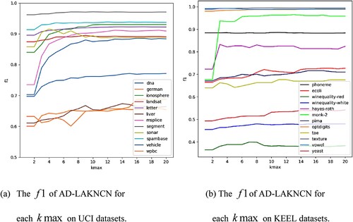
Figures and show that on 24 datasets from the University of California, Irvine (UCI) and Knowledge Extraction based on Evolutionary Learning (KEEL) repositories, except for the sonar dataset, where the accuracy and slowly decreased after reaching a maximum at
, the accuracy and
of the new method increased with the increase of
and fluctuated slightly near the highest point.
Figure 4. The accuracy of AD-LAKNCN for each on 24 real-world datasets.
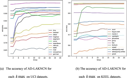
Figure 5. The of AD-LAKNCN for each
on 24 real-world datasets.
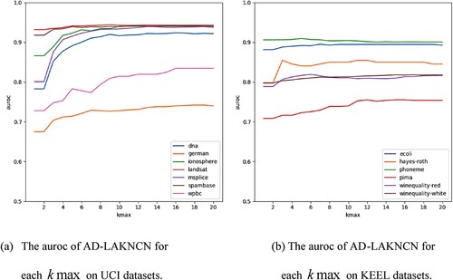
Figures show that on the 13 unbalanced datasets, except for the gmeans of the wpbc dataset, which decreased with the increase in , the kappa, gmeans and AUROC of each dataset appeared to increase with the increase in
.
Figure 6. The kappa of AD-LAKNCN for each on 13 unbalanced real-world datasets.
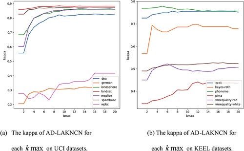
Figure 7. The gmeans of AD-LAKNCN for each on 13 unbalanced real-world datasets.
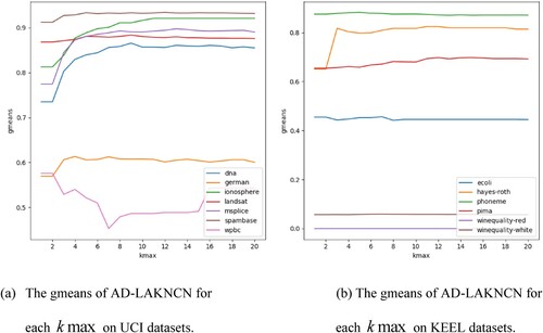
Figure 8. The AUROC of AD-LAKNCN for each on 13 unbalanced real-world datasets.
From the above experiments, the following observations can be made: (1) In most cases, AD-LAKNCN can achieve the best performance when . (2) Selecting a larger
does not reduce the performance. (3) AD-LAKNCN is insensitive to the choice of
and has excellent classification performance.
4.5. Analysis of computational complexity
To explore the computational complexity of the new method, we further analysed the increase in the computational cost of the new method compared with those of KNN and KNCN.
We specify the following notation related to in the computational complexity: ,
,
and
denote the number of training sets, dimensions, maximum
and number of classes, respectively.
The main computational costs of the KNN algorithm are the calculation of the Euclidean distance between the query and all training samples and the determination of the neighbours; combined with the class calculation of the query point, the computational complexity of KNN is . For KNCN, the calculation of each nearest centroid neighbour requires no more than
centroid calculations and distance calculations and
comparison calculations; therefore, the computational cost of the
nearest centroid neighbours is approximately
. Combined with the class calculation of the query point, the computational complexity of KNCN is approximately
.
Table shows the increased computational costs of the new method over those of KNN and KNCN. In step 2, the new method and KNCN execute more computations than KNN when finding the nearest centroid neighbours. In step 3, the new method executes
more computations than KNN and KNCN when selecting the best discrimination class. In step 4, the distance from the query point to the centroid of each
and the ratio of the selected discrimination class in all neighbours need to be calculated when selecting the best
. Compared with those of KNN and KNCN, the increase computation is approximately
. In step 5, the average rank calculation increases the number of computations by
times to determine the class of the query point.
Table 8. The increased computation of the AD-LAKNCN algorithm compared to the KNN and KNCN algorithms.
In addition to the computational complexity analysis above, the running times for classifying all the testing samples on the three UCI datasets and three KEEL datasets are provided in Table when or
. Note that the numbers of the training set, testing set, dimensions and classes are listed in parentheses. All the methods were implemented using Python 3.6.8, and all the experiments were run on a 64-bit Windows 11 operating system with an Intel(R) Core (TM) i5-11600KF central processing unit (CPU) @3.90 GHz with 16 GB of memory.
Table 9. The computational time (s) of actually classifying all the testing samples.
The following conclusions can be drawn from the results in Table : (1) The KNN algorithm achieved the fastest running speed because it is simple. (2) NCN-based methods, including KNCN and AD-LAKNCN, require a somewhat longer running time due to the iterative calculations. (3) Compared with KNCN, the running times of AD-LAKNCN do not increase much.
In summary, since and
are generally smaller than
and
, the higher computational costs of the new method are due to calculating the nearest centroid neighbours, which is the same as in the KNCN, so the new method does not greatly increase the computational costs compared with those of the KNCN. Overall, although the computational costs of the new method increase, they are fully acceptable due to the excellent classification performance of the algorithm.
4.6. Discussion of experimental results
The conclusions of the above experimental results are summarised as follows:
The experimental results on all the evaluation indices show that the proposedAD-LAKNCN method obtains satisfactory classification performance.
The methods (i.e. AD-LAKNCN, LMKNCN and KNCN) that use the NCN method to select the neighbours generally perform better than other KNN-based methods.
The average distance can make full use of the distribution of all neighbours to select the best discrimination class. This is because when selecting a query point discrimination class, using the average distance not only makes the number of discrimination class samples as large as possible but also makes the centroid of the discrimination class as close as possible to the query point.
AD-LAKNCN is insensitive to the choice of
Compared with KNN, KNCN and AD-LAKNCN require more computation due to the iterative calculations.
5. Conclusions
This paper combines the NCN and DC-LAKNN algorithms and uses the number and distribution information of each class of neighbours to propose a new adaptive KNN method called AD-LAKNCN. First, the nearest neighbours of the query point are selected by the NCN method. Next, the discrimination class under each value is determined by comparing the average distances of different classes. Last, the optimal discrimination class for the query point is determined by using the number and distribution information of the discrimination class under each
value.
The new method is compared with nine other KNN-based classification algorithms on 24 real datasets. The experimental results show that the new classifier performs better than other classifiers in terms of accuracy, , kappa, gmeans and AUROC.
The main computational cost of AD-LAKNCN is to iteratively find nearest centroid neighbours, which is the same as KNCN. Compared with the KNN algorithm, the KNCN and AD-LAKNCN require more computation, which limits their application to large-scale data. In future work, we plan to explore parallel computing methods to reduce the computation of finding
nearest centroid neighbours. Moreover, we plan to apply the proposed method to practical applications. For example, we can use average distance as a classification measure to deal with the multilabel classification, which means that some queries should be classified into multiple classes. In addition, the proposed method can be integrated with the other methods for good classification performance.
Disclosure statement
No potential conflict of interest was reported by the author(s).
References
- Alcaĺa-Fdez, J., Ferńandez, A., Luengo, J., Derrac, J., & Garćıa, S. (2011). Keel datamining software tool: Data set repository, integration of algorithms and experimental analysis framework. Journal of Multiple-Valued Logic and Soft Computing, 255–287.
- Chaudhuri, B. B. (1996). A new definition of neighborhood of a point in multi-dimensional space. Pattern Recognition Letters, 17(1), 11–17. doi:10.1016/0167-8655(95)00093-3
- Cover, T. M., & Hart, P. E. (1967). Nearest neighbor pattern classification. IEEE Transactions on Information Theory, 13(1), 21–27. doi:10.1109/TIT.1967.1053964
- Dua, D., & Graff, C. (2017). UCI machine learning repository. Retrieved from http://archive.ics.uci.edu/ml.
- Dudani, A. S. (1976). The distance-weighted k-nearest-neighbor rule. IEEE Transactions on Systems, Man, and Cybernetics, SMC-6(4), 325–327. doi:10.1109/TSMC.1976.5408784
- Gou, J., Du, L., Zhang, Y., & Xiong, T. (2012). A new distance-weighted k-nearest neighbor classifier. Journal of Information and Computational Science, 9(6), 1429–1436.
- Gou, J., Ma, H., Ou, W., Zeng, S., Rao, Y., & Yang, H. (2019). A generalized mean distance-based k-nearest neighbor classifier. Expert Systems with Applications, 115, 356–372. doi:10.1016/j.eswa.2018.08.021
- Gou, J., Qiu, W., Zhang, Y., Xu, Y., Mao, Q., & Zhan, Y. (2019). A local mean representation-based K-nearest neighbor classifier. ACM Transactions on Intelligent Systems and Technology, 10, 1–25. doi:10.1145/3319532
- Gou, J., Sun, L., Du, L., Ma, H., Xiong, T., Ou, W., & Zhan, Y. (2022). A representation coefficient-based k-nearest centroid neighbor classifier. Expert Systems with Applications, 194, 116529. doi:10.1016/j.eswa.2022.116529
- Gou, J., Yi, Z., Du, L., & Xiong, T. (2012). A local mean-based k-nearest centroid neighbor classifier. The Computer Journal, (55), 1058–1071. doi:10.1093/comjnl/bxr131
- Gou, J., Zhan, Y., Rao, Y., Shen, X., Wang, X., & He, W. (2014). Improved pseudo nearest neighbor classification. Knowledge-Based Systems, 70, 361–375. doi:10.1016/j.knosys.2014.07.020
- Guo, G., & Dyer, R. C. (2005). Learning from examples in the small sample case: Face expression recognition. IEEE Transactions on Systems, Man and Cybernetics, Part B (Cybernetics), 35(3), 477–488. doi:10.1109/TSMCB.2005.846658
- Liu, H., & Zhang, S. (2012). Noisy data elimination using mutual k-nearest neighbor for classification mining. Journal of Systems and Software, 85(5), 1067–1074. doi:10.1016/j.jss.2011.12.019
- Ma, H., Gou, J., & Wang, X. (2018). A pseudo nearest centroid neighbour classifier. International Journal of Computational Science and Engineering, 17(1), 55–68. doi:10.1504/IJCSE.2018.094420
- Maloof, M. (2003). Learning when data sets are imbalanced and when costs are unequal and unknown. International Conference on Machine Learning, 21, 1–5.
- Mitani, Y., & Hamamoto, Y. (2006). A local mean-based nonparametric classifier. Pattern Recognition Letters, 27(10), 1151–1159. doi:10.1016/j.patrec.2005.12.016
- Mullick, S. S., Datta, S., & Das, S. (2018). Adaptive learning-based k-nearest neighbor classifiers with resilience to class imbalance. IEEE Transactions on Neural Networks and Learning Systems, 1–13. doi:10.1109/TNNLS.2018.2812279
- Pan, Z., Pan, Y., Wang, Y., & Wang, W. (2021). A new globally adaptive k-nearest neighbor classifier based on local mean optimization. Soft Computing, 25, 2417–2431. doi:10.1007/s00500-020-05311-x
- Pan, Z., Wang, Y., & Pan, Y. (2020). A new locally adaptive k-nearest neighbor algorithm based on discrimination class. Knowledge-Based Systems, 204(1), 106–185. doi:10.1016/j.knosys.2020.106185
- Rastin, N., Taheri, M., & Jahromi, M. Z. (2021). A stacking weighted k-nearest neighbour with thresholding. Information Sciences, 571, 605–622. doi:10.1016/j.ins.2021.05.030
- Śanchez, S. J., & Marqúes, A. (2006). An lvq-based adaptive algorithm for learning from very small codebooks. Neurocomputing, 69(7/9), 922–927. doi:10.1016/j.neucom.2005.10.001
- Śanchez, S. J., Pla, F., & Ferri, J. F. (1997). On the use of neighbourhood-based non-parametric classifiers. Pattern Recognition Letters, 18(11–13), 1179–1186. doi:10.1016/S0167-8655(97)00112-8
- Wang, Q., Zhu, G., Zhang, S., Li, K.-C., Chen, X., & Xu, H. (2021). Extending emotional lexicon for improving the classification accuracy of chinese film reviews. Connection Science, 33(2), 153–172. doi:10.1080/09540091.2020.1782839
- Wei, Z., Liu, W., Zhu, G., Zhang, S., & Hsieh, M.-Y. (2022). Sentiment classification of chinese weibo based on extended sentiment dictionary and organisational structure of comments. Connection Science, 34(1), 409–428. doi:10.1080/09540091.2021.2006146
- Wen, G., Jiang, L., Wen, J., Wei, J., & Yu, Z. (2012). Perceptual relativity-based local hyperplane classification. Neurocomputing, 97, 155–163. doi:10.1016/j.neucom.2012.03.018
- Wu, X., Kumar, V., Quinlan, R. J., Ghosh, J., Yang, Q., Motoda, H., & Steinberg, D. (2008). Multi-view ensemble learning: An optimal feature set partitioning for high-dimensional data classification. Knowledge and Information Systems, 49(1), 1–59. doi:10.1007/s10115-015-0875-y
- Zeng, Y., Yang, Y., & Zhao, L. (2009). Pseudo nearest neighbor rule for pattern classification. Expert Systems with Applications, 36(2), 3587–3595. doi:10.1016/j.eswa.2008.02.003
- Zhang, S., Yu, H., & Zhu, G. (2022). An emotional classification method of chinese short comment text based on electra. Connection Science, 34(1), 254–273. doi:10.1080/09540091.2021.1985968
- Zhu, G., Wang, Q., Liu, H., & Zhang, S. (2020). The mining method of trigger word for food nutrition matching. International Journal of Computational Science and Engineering, 23(3), 205–213. doi:10.1504/IJCSE.2020.111423