Ensemble empirical mode decomposition-based preprocessing method with Multi-LSTM for time series forecasting: a case study for hog prices

Abstract

Drastic hog price fluctuations have a great impact on the welfare of hog farmers, people's living standards, and the macroeconomy. To stabilise the hog price, hog price forecasting has become an increasingly hot issue in the research literature. Existing papers have neglected the benefits of decomposition and instead directly utilise models to predict hog prices by capturing raw data. Motivated by this issue, the authors introduce a new robust forecasting approach for hog prices that combines ensemble empirical mode decomposition (EEMD) and multilong short-term memory neural networks (Multi-LSTMs). First, EEMD decomposes the volatile raw sequence into several smoother subsequences. Second, the decomposed subsequences are predicted separately using a parallel structure model consisting of several LSTMs. Finally, the fuse function combines all the subresults to yield the final result. The empirical results suggest that the proposed method only has minor errors and proves the effectiveness and reliability in experiments on real datasets (2.55207, 4.816, and 0.332 on MAE, MAPE and RMSLE, respectively). Reliable forecasting of hog prices is beneficial to farmers and people to allow optimisation of their production and booking rates and to moderate the adverse effects of potential shocks.

KEYWORDS:

• Hog price forecasting
• EEMD
• LSTM
• machine learning
• deep learning

1. Introduction

China has been consuming pork for at least 5,000 years, and pork consumption has occupied a dominant position in the meat market, accounting for 70% of the total consumption. According to the National Bureau of Statistics data for 2020, China was the largest pork producer, with 41.13 million tons of pork produced and the with the largest imports amounting to 5.15 million tons. The outbreak of COVID-19 also exacerbated the changes in hog prices (Hayes et al., 2020). The Chinese government had to release massive pork reserves to ease the sharp rise in pork prices, which had become elusive, ranging from $28/kg in 2020 to $12/kg in 2021, a decrease of 116% back to the normal level.

Fluctuations pertaining to hog prices affect human lives, social stability, and the revenue of industrial supply chains. The dramatic fluctuations in pork prices have significant impacts on people’s lives because disposable income decreases correspondingly to hog price increases. Hog price fluctuations affect the welfare of the farmers and show changes in the same direction (Fu & Tong, 2021). The instability in hog prices and their practical significance underscore their forecasting importance in the market. Such a drastic change in pork price has aroused the curiosity of scholars. How to reduce the forecasting errors of hog prices to a trustworthy and referenceable range has also been a hot topic in academic circles.

The rapid development of big data and the growing trend of neural network applications have had a profound impact in this field in recent years. Among the neural networks, LSTM has shown a noteworthy ability to process time series. Therefore, a novel approach is required to deal with the forecasting tasks for hog prices, which are characterised by high nonlinearity and volatility.

The ARIMA is a time series method that has been widely used for time series prediction. Ji et al. (Ji et al., 2016) used the ARIMA time series model to predict hog prices and concluded that the required time series was smooth and linear, and Li et al. (Li et al., 2019) utilised ARIMA to analyse and predict prices in Shanghai.

The application of machine learning has also seen a rapid uptake in recent years. SVR is a popular method in the literature. Liu et al. (Liu et al., 2019) began by separating the trend component of the hog price series and predicting the trend component using SVR. Zhang et al. (Zhang et al., 2020) presented a hybrid frame of CEEMD-GA-SVR for hog price forecasting. Gradient boosting decision trees are also involved in this field. Fu and Wu (Fu & Wu, 2020) utilised gradient elevating regression instead of many other competing methods to forecast hog prices with fewer errors.

Subsequently, some scholars discovered that neural networks are also capable of such prediction tasks. Ping et al. (Ping et al., 2010) achieved better results by designing a hybrid method called GM-ANN than applying a single model. Li and Wang (Li & Wang, 2021) proposed the PCA-GM-BP for hog price prediction based on the idea of dimensionality reduction. However, ANN and BP have fixed neurons that cannot be modified to meet the demands of the task, even when some methods are integrated to improve the accuracy. In the face of complex tasks, RNNs are widely acknowledged to be superior to neural networks with fixed neurons. By improving the internal structure, LSTM addresses the weaknesses of the traditional RNNs. Liu et al. (Liu et al., 2021) proposed a firefly algorithm to optimise LSTM for hog price prediction. Ye et al. (Ye et al., 2021) used LSTM to predict the increase or decrease in hog prices after extracting the heterogeneous graph of demand and supply. Table 1 shows a visual listing of the methods.

Table 1. Existing methods used for hog price forecasting.

	Paper	Model	Year	Target	Prediction Interval
Time series method	Ji et al. (Ji et al., 2016)	ARIMA	2016	Hog price	weekly
	Li et al. (Li et al., 2019)	ARIMA	2019	Hog price	monthly
Machine Learning	Liu et al. (Liu et al., 2019)	SVR	2019	Hog price	weekly
	Zhang et al. (Zhang et al., 2020)	CEEMD-GA-SVR	2020	Hog price	monthly
	Fu and Wu (Fu & Wu, 2020)	GBDT	2020	Hog price	monthly
Artificial Neural Network	Ping et al. (Ping et al., 2010)	GM-ANN	2010	Hog price	monthly
	Li and Wang (Li & Wang, 2021)	PCA-GM-BP	2021	Hog price	monthly
Recurrent Neural Network	Liu et al. (Liu et al., 2021)	LSTM	2021	Hog price	weekly
	Ye et al. (Ye et al., 2021)	LSTM	2021	Rise and fall	weekly

The methods listed above did indeed optimise the algorithm significantly. However, even when relatively good results were obtained, existing papers have rarely focused on the characteristics of time series data and applicability of the model. The ARIMA is only useful for dealing with linear time series data and is inefficient when dealing with complex data such as hog prices. Compared with the ARIMA, SVR is capable of handling nonlinear data and training a large number of features, while it is sensitive to missing data in the sample, and finding the hyperplane becomes difficult when the sample size is large. The GBDT can also handle nonlinear data but is less sensitive to missing data. On the other hand, GBDT can bootstrap samples and features efficiently and train multiple trees when there are fewer features but it increases the training time because multiple trees have to be trained. Because of the fixed number of neurons, the ANN is no longer applicable in this field, resulting in poor prediction results. Although LSTM can self-expand neurons and has been shown to be the most effective tool for nonlinear time series prediction, the ability to capture the pattern of the data features is insufficient, and there are deficiencies in the data decomposition. Some of the aforementioned papers also experimentally demonstrate that a combined method is more powerful than a single one. Therefore, designing a hybrid method with the capability of decomposing original data and obtaining an effective and reliable forecast becomes increasingly critical to reduce the degree of difficulty and improve the prediction precision.

In this paper, it is currently more feasible to model the data based on the characteristics of the data itself in terms of hog prices with sharp fluctuations. The EEMD introduced in the proposed method further improves the prediction accuracy of the LSTM by enhancing the ability to capture the data features through a decomposition of the raw sequence. First, ADF and BDS tests are used to determine the nonstationarity and nonlinearity of the hog prices. Second, EEMD is introduced to decompose the raw time series data into a number of intrinsic mode functions (IMFs) and a residue based on the data characteristics. Therefore, the decomposed data, from high frequency to low frequency, become smoother and more stationary. To make decomposed time series data more realistic, EEMD randomly adds white noise to the original time series data to obtain a uniform reference in the time–frequency space. It is an adaptive method of determining the parameters needed to construct the model, and confirms that the model we construct is a good representation of the phenomenon. The main purpose of using EEMD is to relieve the LSTM from its prediction task, although it is sufficiently capable. In other words, for most neural networks, processing smoother time series reduces the training time and yields better results in general. Due to the powerful ability to predict time series and the assistance of EEMD, it is easier for LSTM to analyse the individual trends of several IMFs and to predict the subresults more precisely. The unique gating unit in the LSTM can effectively retain the long-term information, thus enhancing the long-term memory capabilities, which is an advantage that the LSTM enjoys over ANN. Finally, the fuse function combines all the subresults to produce the final prediction. In the model evaluation stage, the proposed model outperforms the other listed methods in regard to accuracy. Meanwhile, LSTM, with open and close access to the information flow, effectively addresses the problem of exploding and vanishing gradients caused by the deepening of the neural network layers. Our major research contributions are as follows:

1. An effective forecasting method for hog prices, named EEMD-MiLSTM, is proposed. The ability of LSTM to handle time series is further enhanced since EEMD assists in determining the necessary parameters of the model and confirms that the model we construct is a good representation of the real phenomenon.

2. A unique parallel structure is designed to allow independent predictions without mutual interferences. By collecting real market data, the experiments also demonstrate the practicality and effectiveness of the proposed method.

3. Using ADF and BDS tests, it is concluded that the hog price follows a time series that is nonstationary and nonlinear.

The paper is organised as follows: Section 2 reviews the related work. Section 3 provides details of the model selection by comparing the RNN and LSTM and the EMD and EEMD. Section 4 gives the details of the experiment. Section 5 suggests the results of the proposed EEMD-MiLSTM method compared with the other state-of-the-art methods and provides a discussion. Finally, Section 6 draws a conclusion and identifies future work.

2. Related works

EMD and EEMD have been proposed to decompose time series data. Cen and Wang (Cen & Wang, 2018) proposed a neural network with a learning rate controlled by CID, and additionally combined it with EEMD for time series data, to predict crude oil. Tan et al. (Tan et al., 2018) developed a runoff forecast model combining EEMD and ANN. Moreover, Mao et al. (Mao et al., 2020) analysed the economic growth fluctuations, incorporating EEMD and causal decompositions. Liu et al. (Liu et al., 2020) introduced a hybrid model called EMD-ELM to predict agricultural product prices. Altınta and Davidson (Altana & Davidson, 2021) enhanced the forecasting accuracy of highway tollgate travelling times with a time series decomposed by EMD. Zhang et al. (Zhang, Qin, et al., 2021a) presented a method of extracting laser ultrasonic defect signals using EEMD. Lin et al. (Lin et al., 2021) suggested a model for the forecasting of financial time series based on EEMD and complexity measures. Zhong et al. (Zhong et al., 2021) proposed a hybrid EEMD and DBN method to address the problem of intermittent fault diagnoses of analogue circuits. Jia et al. (Jia et al., 2021) developed a hybrid method for denoising vibration signals using EEMD. Currently, the combination of EEMD and other models is gradually becoming mainstream, and it is more helpful in extracting the parameters needed for a constructed model during the training phase. Scholars are constantly embroiled in the process of finding the best pairing models with EEMD.

Due to the natural advantages of LSTM, it is frequently used in modelling time series data. LSTM has an optimised recurrent structure that is simpler and more reasonable for processing time series than ANN. Sagheer and Kotb (Sagheer & Kotb, 2018) utilised LSTM to forecast oil production to overcome the difficulty of processing time series. Wang et al. (Wang et al., 2018) introduced ESN-DE, a new RNN Echo State Network optimised by the differential evolution algorithm, to forecast energy consumption. Miao et al. (Miao et al., 2020) delivered a novel LSTM framework for short-term fog forecasting by collecting meteorological element observation data. Mei et al. (Mei et al., 2020) proposed model switching and Bayes model fusion for online real-time bandwidth prediction using a pretrained LSTM model. Sangiorgio and Dercole (Sangiorgio & Dercole, 2020) suggested that LSTM is robust for multistep forecasting of chaotic time series. Li et al. (Li et al., 2020) fused neighbourhood rough sets and LSTM to build a hybrid model for rainfall runoff prediction. In addition, Yan et al. (Yan et al., 2021) introduced an effective compression algorithm for real-time transmission data based on LSTM and XGBoost. Wu et al. (Wu et al., 2022) presented an S_I_LSTM stock price prediction model using a combination of traditional and nontraditional data sources. Additionally, K.E. ArunKumar et al. (ArunKumar et al., 2021) compared three traditional RNN models, including LSTM, to forecast COVID-19 cases, confirming the effectiveness of LSTM for processing time series data. Cai et al. (Cai et al., 2022) used two parallel LSTMs as original traffic feature extraction algorithms based on real datasets. Peng et al. (Peng et al., 2022) introduced the attention mechanism into LSTM for energy consumption prediction. Zhou et al. (Zhou et al., 2021) utilised an LSTM-based model to analyse nonlinear features in complex industrial processes for key variable predictions. Zhang et al. (Zhang, Zhang, et al., 2021b) first denoised the electroencephalography data collected from 30 medical staff and proposed a CNN and LSTM to check medical staff fatigue. Li et al. (Li et al., 2022) embedded LSTM into a model called STLAT to predict stock movements. Tang et al. (Tang et al., 2022) utilised LSTM for anomaly detection of multidimensional time series data. Huan et al. (Huan et al., 2022) proposed a text classification model based on CNN and Bi-LSTM.

There is a large amount of literature on price volatility and various objects. However, only a handful of studies focus on hog price forecasting but do not deal with the data itself, and there is even less research on hog price prediction using component decomposition and deep learning methods. Our study contributes to this area. Among the above methods, EEMD greatly improves the performance of the algorithm and obtains good experimental results. Furthermore, LSTM demonstrates a strong ability to handle time series. Inspired by the fact that hybrid methods outperform single methods, we propose a hybrid method EEMD-MiLSTM for predicting hog prices. The hybrid prediction method, EEMD-MiLSTM, for hog prices is based on ensemble empirical mode decomposition, and the long short-term memory neural network is introduced in detail as follows.

3. Methodology

Due to the characteristics of hog prices and the ability to obtain more accurate forecasting results, a hybrid model, EEMD-MiLSTM, for hog price forecasting is developed.

3.1. Recurrent neural network (RNN)

Sequences in price predictions have a large number of long-term dependencies, which traditional neural networks cannot handle. This is a problem that RNNs can solve. An RNN is a neural network with loops that allows for information persistence. The RNN has a feedback mechanism that allows it to easily update the weight or residual value of the previous step. The feedback mechanism is ideal for time series forecasting. The RNN can learn to predict time series by extracting rules from historical data. For price predictions, the order of the data is important. The earlier the data are input, the smaller the proportion of the whole sequence, and if a sequence is long, RNN will “forget” the earlier data. This also means that RNN can only undertake the task of short-term prediction and does not perform well. Unfortunately, at this increasing interval, the RNN loses the ability to gain information that has been previously connected . The operating structure is shown in Figure 1.

Figure 1. RNN Structure with the Unfold Version.

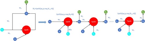
Here, H_t is decided by two factors, x_t and H_t-1, as shown in Equation (1(1) $H_t=\tanh (w_x{x}_t+w_h{H}_{t-1}+b)$(1) ). (1) $H_t=\tanh (w_x{x}_t+w_h{H}_{t-1}+b)$(1)

However, RNNs, like other deep neural networks, are obviously subject to exploding gradients and vanishing gradients. (2) $\begin{array}{rl}\mathrm{\Delta }W& =-\eta \frac{\mathrm{\partial }S}{\mathrm{\partial }{Y}_{predict}}\ast \mathrm{\partial }\frac{Y_{predict}}{\mathrm{\partial }{H}_k}\ast \frac{\mathrm{\partial }{H}_k}{\mathrm{\partial }{H}_{k-1}}\ast \dots \dots \ast \frac{\mathrm{\partial }{H}_2}{\mathrm{\partial }{H}_1}\ast \frac{\mathrm{\partial }{H}_h}{\mathrm{\partial }W}\end{array}$(2) (3) $\begin{array}{rl}\frac{\mathrm{\partial }{H}_k}{\mathrm{\partial }{H}_{k-1}}& ={\tanh }^{\mathrm{\prime }}(w_x{x}_k+w_h{H}_{k-1}+b)\ast W_h\end{array}$(3)

Here, the derivative of tanh falls in the interval from 0 to 1, as shown in Equations (2(2) $\begin{array}{rl}\mathrm{\Delta }W& =-\eta \frac{\mathrm{\partial }S}{\mathrm{\partial }{Y}_{predict}}\ast \mathrm{\partial }\frac{Y_{predict}}{\mathrm{\partial }{H}_k}\ast \frac{\mathrm{\partial }{H}_k}{\mathrm{\partial }{H}_{k-1}}\ast \dots \dots \ast \frac{\mathrm{\partial }{H}_2}{\mathrm{\partial }{H}_1}\ast \frac{\mathrm{\partial }{H}_h}{\mathrm{\partial }W}\end{array}$(2) ) and (3(3) $\begin{array}{rl}\frac{\mathrm{\partial }{H}_k}{\mathrm{\partial }{H}_{k-1}}& ={\tanh }^{\mathrm{\prime }}(w_x{x}_k+w_h{H}_{k-1}+b)\ast W_h\end{array}$(3) ). When the result after its multiplication with w_h is less than 1, the result of successive multiplications eventually converges to 0, causing the gradient to vanish as the number of cycles increases. When the result is greater than 1, the gradient explodes.

3.2. Long short-term memory neural network (LSTM)

LSTM is an RNN variant (Horochreiter & Schmidhuber, 1997). In comparison with RNN, LSTM has the advantage of addressing the problem of gradient vanishing and gradient explosion. After deliberate optimisation, LSTM eliminates the problem of long-term dependency, remembering that long-term information is in practice the default behaviour of LSTM, rather than the capability to obtain it at a high cost.

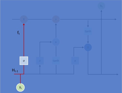
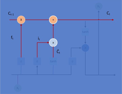
Figure 2 depicts the improvement of LSTM over the recurrent structure of RNN. It has five interacting elements, including 3 sigmoid layers and 2 tanh layers. As shown in Figure 3 and Equation (4(4) $f_t=\sigma (w_f\ast [h_{t-1},x_t]+b_f)$(4) ), the first step in the LSTM is to decide what information will be discarded from the cell state. This decision is made through a layer called the “forget gate”. Because the sigmoid can return a value between 0 and 1, it can gate and control the proportion of information flowing out, with 0 representing complete forgetting and 1 representing complete retention. (4) $f_t=\sigma (w_f\ast [h_{t-1},x_t]+b_f)$(4)

Figure 2. LSTM whole structure.

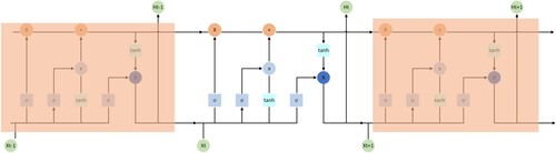
Figure 3. LSTM Structure Step 1.

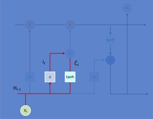
As shown in Figure 4 and Equation (5(5) $\begin{array}{rl}{i}_t& =\sigma (w_i^{\ast }[h_{t-1},x_t]+b_i)\\ {\hat{C}}_t& =\tanh (w_c^{\ast }[H_{t-1},x_t]+b_c)\end{array}$(5) ), this step determines which information is required and which needs to be updated. First, the sigmoid function in the “input gate layer” determines the values it will update. Then, the tanh function can control the direction of information increase or decrease, as well as control the value between −1 and 1. (5) $\begin{array}{rl}{i}_t& =\sigma (w_i^{\ast }[h_{t-1},x_t]+b_i)\\ {\hat{C}}_t& =\tanh (w_c^{\ast }[H_{t-1},x_t]+b_c)\end{array}$(5)

Figure 4. LSTM Structure Step 2.

The period’s state of value C_t will be converted from C_t-1 multiplied by ft. This step determines the information that needs to be discarded. As shown in Figure 5 and Equation (6(6) $C_t=f_t^{\ast }{C}_{t-1}+i_t^{\ast }{\hat{C}}_t$(6) ), i_t and C_t are multiplied to obtain the new memory part of this period. The two are added together to obtain the new state value C_t. (6) $C_t=f_t^{\ast }{C}_{t-1}+i_t^{\ast }{\hat{C}}_t$(6)

Figure 5. LSTM Structure Step 3.

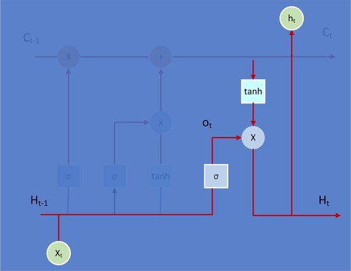
Finally, as shown in Figure 6 and Equation (7(7) $\begin{array}{rl}{o}_t& =\sigma (w_o^{\ast }[h_{t-1},x_t]+b_o)\\ H_t& =o_t^{\ast }\tanh (C_t)\end{array}$(7) ), the output gate determines which part of the information will be output. A sigmoid layer is applied to determine which part of the cell state will be output. It then takes the cell state and processes it through tanh. The two are multiplied together to obtain the new state value H_t. It only outputs the part that determines the output. (7) $\begin{array}{rl}{o}_t& =\sigma (w_o^{\ast }[h_{t-1},x_t]+b_o)\\ H_t& =o_t^{\ast }\tanh (C_t)\end{array}$(7)

Figure 6. LSTM Structure Step 4.

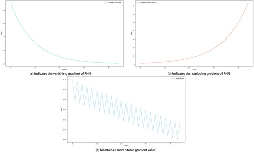
Repeat steps 1–4 until the loop stops and the model ends its operation. The three Equations (8) to (10) explain the exploding and vanishing gradient problem. (8) $\begin{array}{rl}\mathrm{\Delta }W& =-\eta \frac{\mathrm{\partial }S}{\mathrm{\partial }{Y}_{predict}}\ast \frac{\mathrm{\partial }{Y}_{predict}}{\mathrm{\partial }{H}_k}\ast \frac{\mathrm{\partial }{H}_k}{\mathrm{\partial }{C}_{k-1}}\dots \dots \frac{\mathrm{\partial }{C}_2}{\mathrm{\partial }{C}_1}\ast \frac{\mathrm{\partial }{C}_1}{\mathrm{\partial }W}\end{array}$(8) (9) $\begin{array}{rl}\frac{\mathrm{\partial }{C}_k}{\mathrm{\partial }{C}_{k-1}}& =\frac{\mathrm{\partial }{f}_k}{\mathrm{\partial }{C}_{k-1}}\ast C_{k-1}+f_k+\frac{\mathrm{\partial }{i}_k}{\mathrm{\partial }{C}_{k-1}}\ast u_k+\frac{\mathrm{\partial }{u}_k}{\mathrm{\partial }{C}_{k-1}}\ast i_k\end{array}$(9) (10) $\begin{array}{rl}& ={\sigma }^{\mathrm{\prime }}(w_f^{\ast }[H_{k-1},x_k])\ast w_f^{\ast }{O}_{k-1}\ast {\tanh }^{\mathrm{\prime }}(C_{k-1})\ast C_{k-1}\\ & +f_k\\ & +O^{\mathrm{\prime }}(w_h^{\ast }[H_{k-1},x_k])\ast w_u^{\ast }{O}_{k-1}\ast {\tanh }^{\mathrm{\prime }}(C_{k-1})\ast u_k\\ & +O^{\mathrm{\prime }}(w_i^{\ast }[H_{k-1},x_k])\ast w_i^{\ast }{O}_{k-1}\ast {\tanh }^{\mathrm{\prime }}(C_{k-1})\ast i_k\end{array}$(10)

In this case, the sum of these four items is either greater than or less than 1. In other words, unlike RNN, which keeps a constant value in loops, only one of two scenarios occurs in each loop. Figure 7 shows that when compared to two RNN situations, the LSTM appears to be more stable after 40 rounds of the loop.

Figure 7. Comparison of three conditions.

In this figure a indicates the vanishing gradient of RNN. In this figure b indicates the exploding gradient of RNN. In this figure c maintains a more stable gradient value.

3.3. Empirical mode decomposition (EMD)

Huang et al. (Huang et al., 1998) proposed empirical mode decomposition, an adaptive and highly efficient time series decomposition method capable of decomposing nonlinear and nonstationary data. The goal of the EMD is to decompose a signal into a sum of simple components according to the Fourier series. The original sequence should satisfy the following assumptions: 1) the data have greater than or equal to two extremes; 2) the characteristic time scale is defined by the time interval between extremes; and 3) if the data have no extremes at all and only inflection points, it can be differentiated one or more times. These components, unlike Fourier series, do not need to be equipped with simple sinusoidal functions but only have meaningful local frequencies. The key part is that any complex dataset can be decomposed into IMFs based on the local characteristic time scale.

3.4. Ensemble empirical mode decomposition (EEMD)

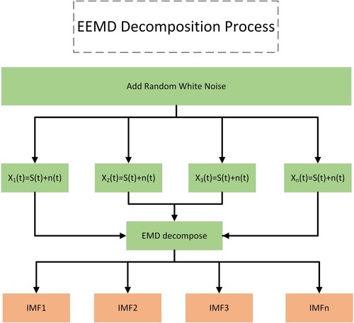
One of the biggest problems with the EMD is mode mixing, which is a defined IMF that consists of neither signals of widely disparate scales, nor signals of similar scales residing in the different IMF components. Huang believes that mode mixing is primarily caused by the intermittent phenomenon, which is frequently caused by abnormal time factors such as intermittent signals, interference signals and noise. When there are anomalous events in the signal, it will inevitably affect the selection of extreme points, causing the distribution of the extreme points to be uneven and thus affecting IMF selection. In complex realistic scenarios, abnormal events are difficult to avoid, making it difficult for the EMD to meet the requirements. To address this problem, Wu and Huang (Wu & Huang, 2009) proposed a new ensemble empirical mode decomposition that added white noise to uniformly populate the entire time–frequency space with the constituting components of the different scales.

The principle of EEMD-MiLSTM, a new hybrid prediction method based on ensemble empirical mode decomposition and the long short-term memory neural network, is introduced in detail. First, the proposed method introduces EEMD to decompose the raw hog price sequence into several smoother subsequences and determines the necessary parameters for the built model. The decomposed subsequences are then predicted separately using a parallel structure model composed of several LSTMs. Finally, the fuse function combines all the subresults to yield the final result.

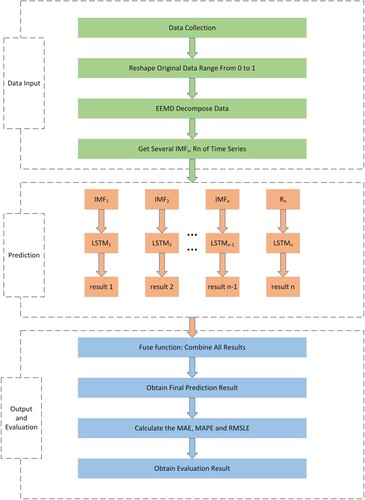
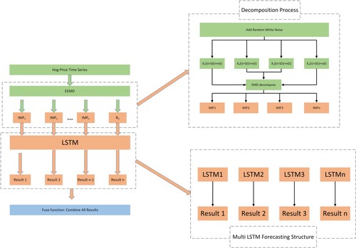
Figure 8 depicts three stages of the proposed EEMD-MiLSTM prediction method. The three stages are data input, model prediction and model evaluation. There are four steps in the data input and the model evaluation, while there are three steps in the model prediction. The EEMD-MiLSTM prediction model is described in detail below:

1. The real hog prices are collected from the Brick Agricultural database. The raw hog price time series data are preprocessed to ensure that the time series data format meets the format requirements of EEMD decomposition.

2. To decompose the input data more smoothly, EEMD decomposes it into several subsequences ranging from high to low frequencies. These subsequences can be expressed as IMF₁, IMF₂ … .IMF_n.

3. It is ensured that the prediction process is clean and uncontaminated and that the results of each prediction are independent and do not interfere with each other. Each subsequence is sent to LSTM for training. These independent LSTMs are named LSTM_1, LSTM₂ … LSTM_n. These n LSTMs are used to predict n subsequences to obtain subresult₁, subresult₂ … subresult_n. The intrinsic laws of each subsequence are fully considered, and the subresults are obtained through the joint prediction of multiple LSTMs.

4. It is crucial to combine the n independent subresults predicted by the n independent LSTMs. The role of the fuse function is to combine several subresults into a final prediction result. Given the importance of each subsequence, we assign equal weights to each subsequence and sum their results with the fuses function to obtain the final prediction result.

5. Finally, the errors between the predicted and true values are calculated using three popular error evaluation metrics: MAE, MAPE and RMSLE. These values are obtained and can be used to evaluate the superiority of the prediction performance.

Figure 8. Flowchart of EEMD-MiLSTM.

4. Experiments

The experiments were conducted on a CPU i5, using Python version 3.7 and Keras 2.4.3 on Windows 10.

4.1. Data resource

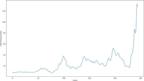
The real pork prices are collected from the Brick Agricultural database to verify the robustness of the proposed EEMD-MiLSTM. The last part of Figure 9 depicts some anomalies that occurred with a steep rise in hog prices during the COVID-19 outbreak. The hog price in the Chinese agricultural market is strongly affected by a variety of objective factors, making it particularly nonstationary and difficult to forecast. In the following section, ADF and BDS tests will be applied to test the stability and nonlinearity, and the conclusions drawn are also consistent with the characteristics of hog prices. Additionally, it is difficult for scholars to design a suitable model.

Figure 9. Hog Price Trends.

4.2. Hog price fluctuation rules

4.2.1. I. ADF test

Table 2 shows the results of using the ADF method to examine the stability of the monthly hog price. The ADF statistic value is −0.479, which is greater than the critical values of −3.46, −2.87 and −2.57 at the three significance levels, and the P value of the companion probability of the T test value is 0.8917 at the 1% significance level. Therefore, the original hypothesis (that the hog price is nonstationary) is not rejected, and a unit root exists, indicating that the hog price is nonstationary.

Table 2. ADF test results for the monthly hog price series.

	T test value	P Value
ADF statistic value	−0.479	0.8917
1% of level critical value	−3.46	–
5% of level critical value	−2.87	–
10% of level critical value	−2.57	–

4.2.2. II. BDS test

The BDS method is used to determine whether the monthly hog prices have nonlinear characteristics. The test results are shown in Table 3. The Z statistic obeys the standard normal distribution with the highest dimension of 6 and is the restrictive distribution of the BDS statistic, with P < 0.01. At 1%, the probability of passing the original hypothesis at the significance level is small, so the original hypothesis (that the hog price is linear) is rejected, and the hog price shows nonlinearity, as derived from the analysis of the results.

Table 3. BDS test results for monthly hog price series.

			dim
	2	3	4	5	6
Z statistic	32.77	33.99	35.73	38.56	42.70
P value	0	0	0	0	0

4.3. Data preprocessing

The main purpose of normalisation is to reduce the processing difficulty of the model and make the model training faster and more accurate. Normalisation facilitates the model finding the optimal solution via gradient descent and improves the accuracy with less loss. Furthermore, the tolerance for outliers is increased accordingly. The formula is represented as Equation (11(11) $x^{\mathrm{\prime }}=\frac{x-min(x)}{max(x)-min(x)}$(11) ). (11) $x^{\mathrm{\prime }}=\frac{x-min(x)}{max(x)-min(x)}$(11)

4.4. EEMD decomposition process

EEMD randomly adds white noise with a mean of 0 to the original data to solve the problem of model mixing. Since zero-mean noise is added, the noises cancel each other out after multiple averaging. The effects of the EEMD decomposition are that the added white noise series cancel each other out in the final mean of the corresponding IMFs; the mean IMFs stay within the natural dyadic filter windows, significantly reducing the possibility of mode mixing and preserving the dyadic property. The following is a brief overview of the decomposition process:

1. Initialise the parameter by setting the number of EMD decompositions to m and the standard deviation of the introduced white noise to a;

2. To obtain the new sequence, add a random white noise sequence n(t) with a zero mean and standard deviation a to the original signal x(t) several times;

3. Find all the extreme points of the signal x(t);

4. Fit the envelopes max(t) and min(t) of the upper and lower extreme value points with three times the spline curve, and find the average of the upper and lower envelopes m(t) in x(t) by subtracting it: h(t) = x(t)-m(t);

5. Determine whether h(t) meets the predetermined criterion for IMF;

6. If not, replace x(t) with h(t), and repeat the above steps until h(t) meets the criterion. h(t) is the IMF_CK(t) to be extracted;

7. Repeat (1)-(6) n times;

8. Average the corresponding IMF components to eliminate the effect of multiple white noises on the true IMF. Finally, the j_th IMF, denoted by IMF_j, can be expressed as follows: (12) $x(t)=\sum _{j=1}^{k}IM{F}_{ij}(t)+r(n)$(12) where IMF_ij denotes the j_th IMF, the i_th time. The greater N is, the closer the sum of the Gaussian white noise added to the IMF is to 0.

9. (9) To eliminate the effect of white noise, the EMD decomposition results are integrated and averaged, and the final results are obtained as shown in Figure 10 and Equation (13(13) $C_j(t)=\frac{1}{m}\sum _{i=1}^{m}C-ij(t)$(13) ). (13) $C_j(t)=\frac{1}{m}\sum _{i=1}^{m}C-ij(t)$(13)

Figure 10. EEMD Decomposition Process with the help of EMD.

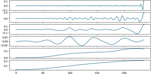
Each IMF becomes more stable than the original data series. The degree of volatility decreases gradually across IMFs. The average period increases sequentially, and the general trend increases as well, with the EMD and EEMD decompositions moving in roughly similar directions. As illustrated in Figures 11,12, the penultimate sequence decomposed by EEMD is more stable than EMD. The last IMF in the EMD and EEMD decomposition graphs is gentler than the first IMF, and it is obvious that the lower subgraph is milder. The more smoothly the time series is decomposed, the more accurate the prediction in the LSTM.

Figure 11. The EMD Decomposition Graph of the Original Series.

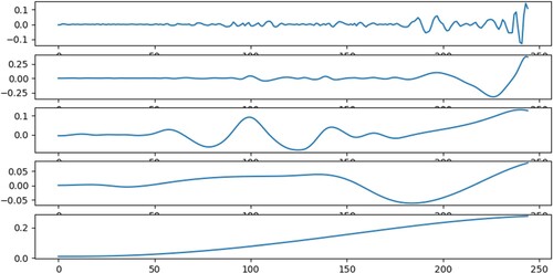
Figure 12. EEMD Decomposition Graph of the Original Series.

4.5. LSTM prediction

To predict price, the IMFs obtained from EEMD are put into LSTM. Here, in the EEMD-MiLSTM hybrid model, we set epochs  = 100, batch size = 16, validation_split = 0.1, train times = 6, and whole rounds  = 600 (5 IMFs plus 1 residue). In addition, a single LSTM is trained with epoch = 600, batch size = 16, and validation_split = 0.1 (training dataset:test dataset = 9:1, as with the other methods). The mean squared error (MSE) is the loss function, and its formulation is shown as Equation (14(14) $MSE=\frac{1}{n}\sum _{i=1}^n{(y_{ti}-y_{pi})}^2$(14) ). (14) $MSE=\frac{1}{n}\sum _{i=1}^n{(y_{ti}-y_{pi})}^2$(14)

Adam is selected as the optimiser function to reduce the training time. Each subsequence is sent to the LSTM to yield a prediction subresult. After receiving all the subresults, the fuse function produces a final prediction result by fusing these subresults, as shown in Figure 13.

Figure 13. Structure and Process of EEMD-MiLSTM Model.

4.6. Complexity and overhead analysis

As previously stated, the LSTM has four layers: the forget gate, input gate, output gate and cell gate. Then, the number of parameters is shown in Equation (15(15) $\mathrm{Number}\mathrm{\_}\mathrm{of}\mathrm{\_}\mathrm{weight}=4\ast \mathrm{Hidden}\mathrm{\_}\mathrm{size}\ast (\mathrm{Input}\mathrm{\_}\mathrm{size}+\mathrm{Bias}+\mathrm{Output}\mathrm{\_}\mathrm{size})$(15) ). (15) $\mathrm{Number}\mathrm{\_}\mathrm{of}\mathrm{\_}\mathrm{weight}=4\ast \mathrm{Hidden}\mathrm{\_}\mathrm{size}\ast (\mathrm{Input}\mathrm{\_}\mathrm{size}+\mathrm{Bias}+\mathrm{Output}\mathrm{\_}\mathrm{size})$(15)

Let n be the number of neurons in the layer and m be the number of dimensions. Therefore, the dimension of the forget gate will be n as well (Hidden_size = Output_size). Overall, the total number of parameters will be 4*[{n*(n + m)}+n], and the number after opening the brackets will be 4(nm + n² + n), where n is hidden_size and m is input_size.

4.7. Performance metrics

The mean absolute error (MAE), mean absolute percentage error (MAPE) and root mean squared logarithmic error (RMSLE) are the evaluation functions used in this paper.

I. MAE: MAE is a basic assessment method that reflects the true picture of errors by averaging the absolute errors. Equation (16(16) $MAE=\frac{1}{n}\sum _{i=1}^n|y_{ti}-y_{pi}|$(16) ) suggests the MAE formula. (16) $MAE=\frac{1}{n}\sum _{i=1}^n|y_{ti}-y_{pi}|$(16)

II. MAPE: The MAPE is another evaluation method, similar to the MAE, that considers not only the errors between the predicted and true values but also the ratio between them and whether the model determined by the size of the value is qualified. This method is formulated as shown in Equation (17(17) $MAPE=\frac{1}{n}\sum _{i=1}^n|\frac{y_{ti}-y_{pi}}{y_{ti}}|$(17) ): (17) $MAPE=\frac{1}{n}\sum _{i=1}^n|\frac{y_{ti}-y_{pi}}{y_{ti}}|$(17)

III. RMSLE: The RMSLE that takes into account the situation of the 0 value in the log function. When a small number of data values in the dataset are abnormal, the log function can be used to eliminate the impact on the overall error. As shown in Equation (18(18) $RMSLE=\sqrt{\frac{1}{n}\sum _{i=1}^n{(\log (y_{ti}+1)-\log (y_{pi}+1))}^2}$(18) ), we hereby select RMSLE as another metric. (18) $RMSLE=\sqrt{\frac{1}{n}\sum _{i=1}^n{(\log (y_{ti}+1)-\log (y_{pi}+1))}^2}$(18)

5. Results and discussion

5.1. Competing methods

To demonstrate the superiority of the proposed method, the results of several popular methods using the same data in the experiment are listed here for comparison. Then, the experimental results of each model are then elaborated.

5.1.1. Random Forest (RF)

The RF is an ensemble ML method that consists of many decision trees (Breiman, 2019). Since each decision tree has a different internal structure and information, the reasoning process and results vary. Following the preliminary forecasting results of each tree, the result with the most votes will be accepted.

5.1.2. Extreme gradient boost (XGB)

XGB is a scalable machine learning system for tree boosting (Chen et al., 2016). The XGB, similar to the RF, also consists of many decision trees; however, the XGB first trains a tree, calculates the difference from the true value, and then trains a second tree based on the first tree, adds the predicted value of the first tree, calculates the difference from the true value by minimising the regularised objective functions, and continuously repeats this process. The training process is complete when the criterion or a predetermined number of values is reached.

5.1.3. LightGBM (LGBM)

The LGBM is a different type of GBDT that is a leafwise algorithm (Ke et al., 2017). The LGBM has improved in speed. The LGBM notes that data instances with different gradients play different roles in calculating the information gain, which is called gradient-based one-side sampling. LGBM can then find the best split point to reduce the training time.

5.1.4. MLP

MLP is an abbreviation for multilayer perceptron, a popular neural network that contains an input layer, several hidden layers, and an output layer. MLP is a forward-structured ANN that overcomes perceptrons’ inability to recognise linearly indivisible data. Therefore, we add MLP and EEMD-MLP as additional comparison methods to increase the diversity of the comparative experiments.

5.1.5. RNN

The RNN was introduced in the previous section and will not be repeated here. We additionally add EEMD-RNN as a comparison method to validate the effectiveness of our proposed method.

The charts above show that the lower values are better.

Table 4 and Figure 14 show that when the MAE, MAPE and RMSLE are considered, LSTM achieves the best outcomes by achieving the lowest errors in the single model comparison, with a reduction of 0.09519–2.32315 on MAE, 0.02–15.806 on MAPE, and 0.00009–0.06973 on RMSLE. Moreover, RNN and MLP attain the second and third best performances, respectively, as we expected. Thus, neural networks have some advantages over machine learning methods for prediction tasks. This also highlights the superiority of the performance of the neural networks, particularly LSTM.

Figure 14. Comparison of the Single Models.

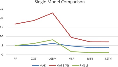
Table 4. Comparison on Test set.

Method	MAE	MAPE (%)	RMSLE
RF	5.19384	16.733	0.05009
XGB	4.87842	18.627	0.06124
LGBM	6.11573	22.804	0.08143
MLP	4.77914	9.45	0.01646
RNN	3.88777	7.018	0.01179
LSTM	3.79258	6.998	0.01170
EEMD-MLP	3.67443	6.544	0.00505
EEMD-RNN	3.03470	5.64	0.00481
EMD-MiLSTM	3.29959	5.714	0.00545
EEMD-MiLSTM	2.55207	4.816	0.00332

There are some reasons for obtaining such results. As previously mentioned, MLP cannot address the problem of long-term dependency as data grow. It is difficult for an MLP with a fixed number of neurons to cope with new changes because it lacks the ability to expand, and cannot perform increasingly difficult tasks. On the other hand, RNNs can self-expand neurons via their recurrent structure to adapt to new changes and improve prediction performance. In comparison with RNN, LSTM contains a special gating unit that enables it to remember and save information for a long time, particularly for information that changes over time. This is why LSTM can reduce the prediction errors even further. A conclusion drawn from the comparison of single methods illustrates the superiority and rationality of LSTM in selecting prediction models.

It is also clear from Table 4 and Figure 15 that the proposed EEMD-MiLSTM outperforms the counterpart. The MAE of the proposed method is 1.12236 lower than that of EEMD-MLP and 0.48263 lower than that of EEMD-RNN. In terms of the MAPE, the proposed method decreases values by 1.728 and 0.824, respectively. The proposed method reduces errors by 0.00173 and 0.00148 for the RMSLE, respectively. It can be clearly seen that MLP and RNN also integrate EEMD, but their performance is still weaker than that of EEMD-MiLSTM. Therefore, the hybrid method comparisons also illustrate the correctness of LSTM in selecting prediction models.

Figure 15. Comparison of the Hybrid Models.

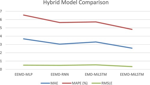
Due to structural flaws, the prediction performance of MLP and RNN is inferior to that of LSTM when compared to single models. However, it is worth noting that, after combining with EEMD, the performance of EEMD-MLP and EEMD-RNN outperforms that of LSTM, with a reduction of 0.11815 and 0.75788 on MAE, 0.454 and 1.358 on MAPE, and 0.00665 and 0.00689 on RMSLE. The reason EEMD-MLP and EEMD-RNN outperform LSTM is that EEMD offers assistance, such as defined parameters, to enhance the MLP's ability to handle time series data, compensate for the lack of dealing with long-term dependency and improve the overall model performance to some extent.

Table 4 and Figure 16 suggest that EEMD-MiLSTM has made a huge contribution to error reduction. The MAE of EEMD-MiLSTM has decreased by 1.24051, MAPE has decreased by 2.812, and RMSLE has decreased by 0.838 when compared with LSTM. Furthermore, it can be clearly demonstrated that LSTM predicts smoother sequences decomposed by EEMD better than LSTM predicts original sequences directly. Meanwhile, the results of EEMD-MLP (MAE = 3.67443, MAPE = 6.544, RMSLE  = 0.505) are superior to those of MLP (4.77914, 9.45, and 1.646, respectively). From the above results, we can conclude that EEMD helps to reduce the model’s prediction errors.

Figure 16. Comparison of Related LSTM Models.

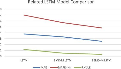
For a variety of reasons, EEMD can assist MLP, RNN and LSTM in improving their performance by decomposing raw data. If data with sharp fluctuations, instability and nonlinearity are predicted directly, it is difficult to understand the internal fluctuation characteristics of the data and achieve the best prediction performance. EEMD is introduced to assist the model in quickly grasping the fluctuation pattern to determine the required model parameters and significantly reduce errors. In addition, EEMD decomposes the original sequence into several smoother subsequences that are put into the models for separate predictions, further reducing the errors. EEMD does help the model greatly reduce the prediction errors. This also substantiates our correct selection of EEMD, which greatly improves the accuracy.

Considering the results, it is clear that the hybrid model combining EEMD and LSTM engenders the smallest errors for MAE, MAPE and RMSLE compared to all the other methods, including LSTM, EEMD-MLP and EEMD-RNN. Figure 17 also provides a visual representation of the methods as well as the predicted results. In terms of accuracy, it also demonstrates the effectiveness and superiority of a combination of EEMD and LSTM, as shown in Table 4 and Figure 17.

Figure 17. Comparison of All Models.

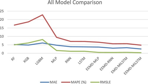
It is experimentally demonstrated that EEMD can improve the model performance by accurately capturing the data characteristics. Meanwhile, with the help of EEMD, LSTM has improved its ability to handle nonlinear and nonstationary data, resulting in lower prediction errors and higher prediction accuracy. Therefore, it can be concluded that the hybrid method EEMD-MiLSTM is the best combination.

6. Conclusion and future work

In this paper, an effective framework of EEMD-MiLSTM with a parallel structure was proposed for hog price prediction. EEMD is introduced to decompose the original sequence into five smoother IMFs and one residual. The subsequences are then sent to LSTM, which enhances the ability to process time series. The fuse function combines all the results to yield the final result. The merits of this hybridisation lies in the fact that the raw time series decomposed by EEMD are stationary and stable, which is beneficial for model training and forecasting to relieve the forecasting pressure of LSTM. The effectiveness and robustness of the proposed model are verified via a comparison with several state-of-the-art models. The MAE, MAPE and RMSLE are 2.55207, 4.816, and 0.332, respectively. Simultaneously, the results can provide informative and reliable advice that can be used to guide the actual production and have a certain practical significance. The volatility of the hog price affects the supply and demand of the hog market. External impacts such as epidemics, policy uncertainty, and African swine have caused hog prices to fluctuate drastically, making it difficult for the government to formulate policies to stabilise the hog market. The hybrid model in this study helps hog farmers to adjust the farming scale, people to adjust their expenditure ratio, and policy-makers to regulate prices to mitigate the impact on the economy.

However, there are still some drawbacks contained in the literature. First, although the added white noise is cancelled out after averaging, there are still some residual noise in the original sequence, which has a minor impact on the prediction accuracy. Second, while LSTM is responsible for calculating the dependence between individual observations in the time series, the performance will be affected when the series is particularly long. On the other hand, the application of CEEMD, a more advanced decomposition method than EMD and EEMD, should be considered in future works.

Declaration of interests

The authors declare that they have no known competing financial interests or personal relationships that could have appeared to influence the work reported in this paper.

Acknowledgement

This research was supported by grants from the National Natural Science Foundation of China (No: 71963019) and the General Program for Public Visiting Scholars of the China Scholarship Council (CSC no: 202008360074). The authors would also like to extend special appreciation to the anonymous reviewers for their invaluable and professional suggestions.

Disclosure statement

No potential conflict of interest was reported by the author(s).