Lithium-ion battery state-of-charge estimation based on a dual extended Kalman filter and BPNN correction

Abstract

It is challenging for a battery management system to estimate the State-Of-Charge (SOC) of batteries. A novel model-based method, using a Dual Extended Kalman Filtering algorithm (DEKF) and Back Propagation Neural Network (BPNN), is proposed to estimate and correct lithium-ion batteries. The results of acceptable SOC estimation are achieved using the DEKF to estimate the battery SOC and simultaneously update model parameters online, while the SOC estimation error is in real-time predicted by the trained BPNN. To further reduce the SOC estimation error, the SOC estimated by the DEKF is corrected by adding the predicted estimation error. The SOC estimation results between the original DEKF and BPNN-based updated DEKF methods under the Federal Urban Driving Schedule (FUDS), the Dynamic Stress Test (DST), the Beijing Dynamic Stress Test (BJDST) and the US06 Highway Driving Schedule are compared. Experimental results show that the SOC error reduces considerably after correcting the estimated SOC. The corrected SOC Root-Mean Square Errors (RMSEs) decrease by an average of seven times compared with the case of no correction. The constant current discharge test verifies the generality and robustness of the proposed method. The modification to the SOC estimation results using ordinary EKF under the above four sophisticated dynamic tests verifies the effectiveness of the proposed method.

KEYWORDS:

• State-of-charge
• lithium-ion battery
• neural network
• state-of-charge correction
• dual extended Kalman filter

1. Introduction

Due to the depletion of fossil energy and environmental pollution, developing the utilisation of clean renewable energies has been imperative. In the field of transportation, governments around the world have begun to plan the development of electric vehicles (EVs). Lithium-ion batteries, as clean and reusable energy, have become the most promising energy storage devices for EVs because of their high power and energy density, long lifespan, excellent design flexibility and no memory effect (Ibrahim & Jiang, 2021; Jwa et al., 2020; Wang et al., 2022; Zhang et al., 2021). The hard operating conditions in EVs necessitate monitoring the states of battery cells, for example, state-of-charge (SOC) (Kim et al., 2021; Wang et al., 2020), state-of-energy (SOE) (An et al., 2022) state-of-health (SOH) (Ezemobi et al., 2022; She et al., 2021) and state-of-power (SOP) (Zhang et al., 2022) and charging capacity abnormality (Wang, Tu, et al., 2022). The SOC is equivalent to the fuel indicator of the internal combustion engine vehicle, which is defined as the ratio of the remaining to the nominal capacity. Accurate SOC estimation can not only provide the driver with information about the remaining mileage but also prevent the batteries from over-discharge or over-charge. It is unfortunate that the SOC cannot be measured directly and can be only estimated by estimation algorithms combined with the measured battery current, voltage and temperature.

References (Adaikkappan & Sathiyamoorthy, 2022; Qays et al., 2022; Sun et al., 2022; Wang et al., 2020; Xiong et al., 2017) comprehensively reviewed present SOC estimation methods, which can be roughly categorised into three types. The former one, the conventional method: mainly includes coulomb counting (CC) or ampere-hour integral method and the open-circuit voltage (OCV) method. The CC method is the most often used in practical battery management systems owing to the ease to implement it. However, the measuring error of the current sensor and the incorrect initial SOC value highly influences its accuracy. In real applications, a periodic calibration for the current sensor and the SOC at present needs to be designed in order to prevent a cumulative error. There is no doubt that such calibration increases the complexity of the CC method. The basis of the OCV method is the functional relationship between the OCV and SOC. Although the OCV-SOC relationship can be accurately determined offline, the OCV cannot be measured in real time because the batteries need to rest for several hours to stabilise the OCV. Thus, it is incapable of estimating the SOC when we drive EVs.The second type, the pure data-driven method: this method treats the battery as a “black box”, by which the relationship between the battery SOC and its related factors can be described. The related factors include the battery voltage, current and environment temperature. It can be used to predict the SOC after being trained by learning algorithms (Ephrem et al., 2018; Hu et al., 2022; Ma et al., 2021; Mao et al., 2022; Tian et al., 2021; Wang, Song, et al., 2021; Wang, Xu, et al., 2022) combined with appropriate training samples. For example, in Reference (Ephrem et al., 2018), a deep feedforward neural network was designed for battery SOC estimation at various ambient temperature conditions. The network can map measurable quantities directly to SOC and achieve competitive estimation performance with the mean absolute error (MAE) below 1%. In Reference (Ma et al., 2021), the battery SOC and SOE were simultaneously estimated by a long short-term memory (LSTM) deep neural network (DNN). The estimation performance with MAEs of ∼1% under various working conditions was achieved. Hu et al. (2022) developed a DNN to predict the SOC of LiFePO₄ batteries in the charging stage. Likewise, a DNN was established by Tian et al. (2021) for estimating the SOC of LiFePO₄ batteries. Considering ordinary neural networks easily falling into local extreme points which result in low estimation accuracy, Mao et al. (2022) proposed a particle swarm optimisation algorithm based on Levy’s flight strategy to optimise the weights and thresholds of neural networks. In Reference (Wang, Ye, et al., 2021), the least squares support vector machine (LSSVM) and recurrent neural network were designed for co-estimation of the battery SOC and capacity. However, whether for the estimation techniques based on neural networks, SVM or other learning algorithms, the SOC estimation accuracy is highly influenced by the training dataset, and deteriorates when the trained “black box” works on untrained datasets. Lastly, the latter type and the model-based method: this method usually utilises adaptive filtering algorithms on the basis of a battery model that can describe battery inside behaviour to estimate SOC. Such estimation methods are suitable for applications under complex working conditions since they can implement self-correction through a closed-loop system. The most popular battery model is the equivalent circuit model (ECM), while the most frequently used filtering algorithm is the Kalman filter family (Shrivastava et al., 2019). For example, in Reference (Zheng et al., 2013), on the basis of a second-order RC circuit model, an extended Kalman filter (EKF) was proposed to estimate the battery SOC. However, in the iterative steps, the noise covariance of EKF remains fixed. If an improper noise covariance is used, it may lead to a significant error or even wrong results. To address the issue, in References (Chen et al., 2022; Duan et al., 2020; He et al., 2021; Peng et al., 2021; Sun et al., 2020; Xiong et al., 2013), improved or adaptive EKF was proposed to adaptively adjust the state and measurement noise covariance. Furthermore, unscented Kalman filter (UKF) and their variants (He et al., 2013; Lv et al., 2020; Zhang et al., 2020), as well as nonlinear observers (Kim et al., 2015; Qiao et al., 2017) were employed to estimate the battery SOC. Besides the estimation algorithm, the battery model accuracy also influences the accuracy of SOC estimation. To improve the accuracy of the battery model, thus further enhancing the SOC estimation accuracy, some techniques based on double/dual filters or joint estimators (Duan et al., 2020; Guo et al., 2016; Guo et al., 2019; Pavkovic et al., 2017; Xing et al., 2022) were proposed for estimating the SOC and simultaneously updating the model parameters online. Moreover, fractional-order battery models (FOMs) are gradually popular in recent years and have been used to improve the accuracy of battery modelling. In References (Hu et al., 2018; Ling & Wei, 2021; Zhu et al., 2019), various methods combined with FOMs were developed for battery SOC estimation and satisfactory results were obtained. For instance, the battery SOC was estimated by a FOM-based adaptive EKF in Reference (Zhu et al., 2019). The presented algorithm can correct noise covariance, and thus diminish SOC estimation error and the optimal MAE of 0.85% was achieved. The modelling and estimation performances between FOM models and integer-order models were comprehensively compared in Reference (Xiao et al., 2016). The results showed that the FOM increased the modelling and SOC estimation accuracy under complex working conditions but a larger computational burden. Reference (Xiao et al., 2016) comprehensively compared FOM models with integer-order models for battery modelling and SOC estimation. The comparison results showed that the FOM had higher modelling accuracy and faster SOC convergence speed under complex dynamic conditions but a larger computational burden. Although model-based methods achieve satisfactory SOC estimation results, the estimation error has a certain extent, even aggravates if the batteries are operated under complex conditions.

To fully exploit the respective advantages of model-based methods and learning algorithms, this paper proposes a SOC estimation method for lithium-ion batteries based on dual EKF and back propagation neural network (BPNN) correction. The main contributions of this work include (1) We design a novel SOC estimation scheme for lithium-ion batteries. First, acceptable SOC estimation results are achieved using a dual extended Kalman filtering algorithm to estimate the battery SOC and simultaneously update model parameters online. Second, the scheme uses a trained BPNN to predict the real-time SOC estimation error. The SOC estimated by the dual estimators is corrected by adding the predicted estimation error to obtain accurate SOC; (2) We present strict theoretical derivation and calculation procedure of dual EKF for facilitating relevant researchers to understand and master it; and (3) The effectiveness and accuracy of the proposed method are demonstrated under four sophisticated dynamic tests, i.e. the FUDS, DST, BJDST and US06. The proposed method has less SOC estimation error than model-based or pure data-driven methods.

The rest of this paper is organised as followed. In Section 2, data sources and experiments are described. Section 3 presents battery modelling including equivalent circuit model, OCV-SOC relationship determination and model parameter identification by adaptive genetic algorithm. Section 4 presents the SOC estimation by dual EKF and SOC correction by BPNN. Experimental results under four sophisticated dynamic tests are analysed in Section 5. Section 6 concludes this paper.

2. Experiments

The data for validating the proposed method in this paper are open and provided by a battery research team at the University of Maryland. INR18650-20R lithium-ion battery manufactured by Samsung is regarded as a test object and its specifications are listed in Table 1. The team conducted various dynamic tests at room temperature (25°C) using a battery test platform, which mainly consists of battery control and signal sample system (Arbin BT2000), a constant temperature chamber and a PC with data sample and battery test software. Zheng et al. (2016) described the test platform in detail. The conducted dynamic tests included the Hybrid Pulse Power Characteristic (HPPC), FUDS, DST, BJDST and US06. The battery current and voltage were sampled at the interval of 1 s. These five separate tests are employed for identifying model parameters, establishing the OCV-SOC relationship and validating the proposed method, respectively.

Table 1. The specifications of the lithium-ion battery INR18650-20R.

Cell dimension (mm*mm)	Rated capacity (Ah)	Charge cut-off voltage (V)	Discharge cut-off voltage (V)	Rated voltage (V)	Maximum continuous discharge current (A)
18*65	2	4.2	2.5	3.6	20

2.1. Model identification and OCV-SOC test

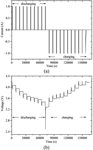
For model parameter identification and OCV-SOC relationship establishment, the HPPC test was conducted. In general, battery model parameters and OCV-SOC relationship are different in the process of battery charging and discharging. Considering the difference between battery charging and discharging, the HPPC test consisted of a discharge HPPC and a followed charge HPPC test. Figure 1(a,b) shows the current and voltage profiles of the HPPC test, respectively. The detailed processes for OCV-SOC relationship establishment and parameter identification are described in Section 3.2 and 3.3, respectively.

Figure 1. The profiles of HPPC test current and voltage.

2.2. Method validation test

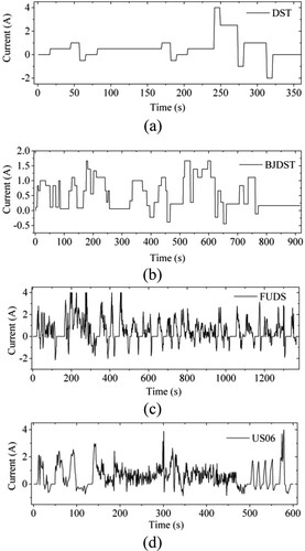
Four sophisticated dynamic tests, namely the DST, BJDST, FUDS and US06 tests, are applied to verify the proposed algorithm for estimating the battery SOC. Figure 2 shows one cycle current profile of each test. In all the current profiles, the positive current denotes battery discharging, while the negative represents battery charging. Figure 2(a–d) shows one cycle current profile of the DST, BJDST, FUDS and US06 tests, respectively. The duration of a completed DST, BJDST, FUDS and US06 cycle is 360, 916, 1372 and 600 s, respectively. The mean currents in one DST, BJDST, FUDS and US06 cycle are 0.533, 0.526, 0.505nd 0.556 A, which lead to a consuming capacity of 0.0533, 0.1338, 0.1925 and 0.0927 Ah, respectively.

Figure 2. The current profiles for method validation: (a) one DST cycle; (b) one BJDST cycle; (c) one FUDS cycle; (d) one US06 cycle.

3. Battery modelling

3.1. Battery model

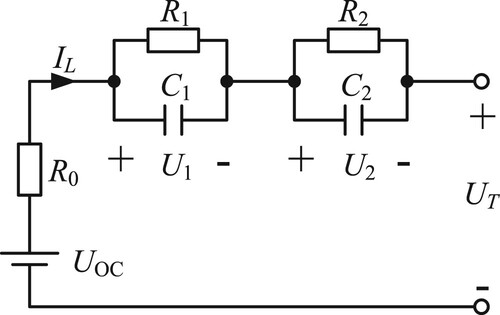
For based-model methods for the battery SOC estimation, an available model is required. Among various equivalent circuits, the second-order RC circuit was widely used and has proved its high accuracy. Therefore, the battery is modelled by the second-order RC circuit in this paper. A schematic diagram of the battery model is shown in Figure 3.

Figure 3. Schematic diagram of the battery model.

For the battery model, the relation equations between battery current, voltage and SOC can be expressed as (1) $\begin{array}{rl}& \{\begin{array}{l}{\displaystyle \frac{\text{d}{U}_1(t)}{\text{dt}}=-\frac{1}{R_1{C}_1}{U}_1(t)+\frac{1}{C_1}{I}_L(t)}\\ {\displaystyle \frac{\text{d}{U}_2(t)}{\text{dt}}=-\frac{1}{R_2{C}_2}{U}_2(t)+\frac{1}{C_2}{I}_L(t)}\end{array}\end{array}$(1) (2) $\begin{array}{rl}& U_T(t)=U_{OC}(t)-R_0{I}_L(t)-U_1(t)-U_2(t)\end{array}$(2) (3) $\begin{array}{rl}& \frac{\text{d}SOC(t)}{\text{dt}}=-\frac{\eta I_L(t)}{C_{\text{p}}}\end{array}$(3) where U₁ and U₂ denote the voltage across the two RC networks, respectively, U_T and I_L are terminal voltage and load current, respectively, U_OC is the OCV of the battery, R₀ is the ohmic internal resistance, R₁, C₁, R₂ and C₂ represent the electrochemical polarisation resistance and capacitance, and concentration polarisation resistance and capacitance, $\eta$ is the coulombic efficiency, while C_p is the rated battery capacity. The discrete-time domain system equation of the battery model can be described as (4) $\begin{array}{rl}& \{\begin{array}{l}{U}_{1,k}={\text{e}}^{\frac{-T_S}{R_1{C}_1}}\cdot U_{1,k-1}+R_1\left(1-{\text{e}}^{\frac{-T_S}{R_1{C}_1}}\right)I_{L,k-1}\\ U_{2,k}={\text{e}}^{\frac{-T_S}{R_2{C}_2}}\cdot U_{2,k-1}+R_2\left(1-{\text{e}}^{\frac{-T_S}{R_2{C}_2}}\right)I_{L,k-1}\end{array}\end{array}$(4) (5) $\begin{array}{rl}& U_{T,k}=U_{OC,k}-R_0{I}_{L,k}-U_{1,k}-U_{2,k}\end{array}$(5) (6) $\begin{array}{rl}& \text{SO}{\text{C}}_k=\text{SO}{\text{C}}_{k-1}-\frac{\eta T_S}{C_{\text{p}}}{I}_{L,k-1}\end{array}$(6) where $T_S$ is the sample time. Many reported literature showed that the time constant (i.e. product of resistance and capacitance) of the RC network in the second-order RC circuit model is much more than 1 s. Then, Equation (4) can be simplified as (7) $\{\begin{array}{l}{U}_{1,k}=(1-\frac{T_S}{R_1{C}_1})U_{1,k-1}+\frac{T_S}{C_1}{I}_{L,k-1}\\ \\ U_{2,k}=(1-\frac{T_S}{R_2{C}_2})U_{2,k-1}+\frac{T_S}{C_2}{I}_{L,k-1}\end{array}$(7)

In Equation (5), $U_{OC,k}$ can be expressed by the function $OCV(SO{C}_k)$. In addition, $OCV(SO{C}_k)$ can be approximately expressed as a linear function by Taylor expansion.

For an accurate description of the behaviour especially when the batteries are operated under complex conditions, the model parameters should be online estimated. By defining $x_k=[SO{C}_k,U_{1,k},U_{2,k}{]}^{\text{T}}$, $u_k=I_{L,k}$, $y_k=U_{T,k}$, ${\theta }_k={\left[R_{0,k},\frac{T_S}{C_{1,k}},\frac{T_S}{R_{1,k}{C}_{1,k}},\frac{T_S}{C_{2,k}},\frac{T_S}{R_{2,k}{C}_{2,k}}\right]}^{\text{T}}$, the model (5)–(7) can be rewritten as (8) $\begin{array}{rl}{x}_k& =A({\theta }_{k-1})x_{k-1}+B({\theta }_{k-1})u_{k-1}\\ & =f(x_{k-1},u_{k-1},{\theta }_{k-1})\end{array}$(8) (9) $\begin{array}{rl}{y}_k& =OCV(x_{1,k})-{\theta }_{1,k}{u}_k-x_{2,k}-x_{3,k}\\ & =g(x_k,u_k,{\theta }_k)\end{array}$(9) where $A({\theta }_k)=\left[\begin{array}{ccc}1& 0& 0\\ 0& 1-{\theta }_{3,k}& 0\\ 0& 0& 1-{\theta }_{5,k}\end{array}\right]$, $B({\theta }_k)=\left[\begin{array}{c}-\frac{\eta T_S}{C_{\text{p}}}\\ {\theta }_{2,k}\\ {\theta }_{4,k}\end{array}\right]$, $x_{i,k}$ and ${\theta }_{i,k}$ are the ith element of $x_k$ and ${\theta }_k$, respectively, and $OCV(\cdot )$ represents the OCV function with respect to SOC.

3.2. Establishment of the OCV-SOC relationship

Determining the relationship between OCV and SOC is an essential procedure of model-based methods to estimate the battery SOC accurately. The OCV-SOC relationship is established by the HPPC test, as there are differences in the OCV-SOC relationship between discharging and charging, as mentioned above. The discharging and charging HPPC tests are conducted to determine the OCV-SOC relationship. That is, in the discharging HPPC test, the battery is first fully charged, thus 100% SOC. Then, it rests for 2 h, and then the terminal voltage is recorded as OCV corresponding to 100% SOC. Next, the battery is discharged for 12 min using a constant current of 0.5 C rate (i.e. the current magnification of 1A for a 2 Ah battery), corresponding to a 10% SOC decrease.

As the next step, it rests for 2 h over again. The terminal voltage is recorded as the OCV corresponding to 90% SOC and repeated the discharge and rest process until the SOC decreases to zero. The recorded 11 OCVs corresponding to SOC from 0% to 100% with an interval of 10% are shown in Figure 4 (see black circle). After the discharging HPPC test, the charging HPPC test starts. First, the battery is charged for 12 min using a constant current of 0.5 C rate, which corresponds to a 10% SOC increase. Then, rest for another 2 h, as the terminal voltage is recorded as the OCV corresponding to 10% SOC. Repeat the charging and rest process, and finish when the SOC reaches 100%. The recorded 11 OCVs corresponding to SOC from 0% to 100% with an interval of 10% are shown in Figure 4 (see red circle).

Figure 4. The OCV-SOC fitting curve. The OCV is the average of the discharging OCV and charging OCV.

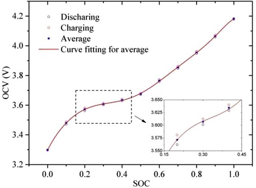
Due to the fact that the end of the discharging HPPC test is the start of the charging HPPC test, they have the same OCV at 0% SOC, as seen in Figure 4 the charging OCV is higher than the discharging OCV. This is a voltage hysteresis phenomenon inside the battery. To minimise the hysteresis effect on the SOC estimation as far as possible, the average of two OCVs is regarded as the OCV in Equation (9), as indicated by the blue star in this same figure.

We use the average OCVs to fit the function of $OCV(SOC)$ using an eighth-order polynomial: (10) $OCV(SOC)=a_0+\sum _{i=1}^8{a}_i\cdot SO{C}^i$(10)

Figure 4 shows the OCV-SOC fitting curve, and Table 2 lists the fitted coefficients. It can be seen from Figure 4 that the average OCVs approach very closely to the fitting curve, and the root-mean-square error (RMSE) between them is only 2.31 mV.

Table 2. Fitted coefficients of the eighth-order polynomial.

Coefficient	value
$a_0$	3.29730
$a_1$	2.48326
$a_2$	−8.76200
$a_3$	31.28446
$a_4$	−129.03774
$a_5$	348.05981
$a_6$	−494.09959
$a_7$	345.30567
$a_8$	−94.35046

3.3. Model parameter identification

There are two purposes for parameter identification. The first is to provide online parameter identification with an appropriate initial value in order to achieve quick convergence of the proposed DEKF. The second is to provide model parameters for the EKF algorithm during the SOC estimation.

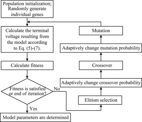
In References (Su et al., 2021) and (Ming et al., 2017), particle swarm optimisation (PSO) and genetic algorithm (GA) were used to identify the parameters in lithium-ion battery equivalent circuit models, respectively. However, both algorithms have a common disadvantage, that is, they are easy to fall into the local optimal solution. Considering the better global searching ability and faster convergence speed of the adaptive genetic algorithm (AGA) by adaptively changing crossover and mutation probabilities, AGA is used to identify the battery model parameters, i.e. R₀, R₁, C₁, R₂ and C₂. At the start of AGA, firstly initialise the population and then generate its individuals, each of which denotes a solution. Genes in GA represent the elements that compose the individuals. For the application of AGA to parameter identification, the model parameter vector corresponds to each individual and thus it is composed of five genes representing the values of (R₀, R₁, C₁, R₂ and C₂). The population continues to evolve until an optimal individual is produced, minimising the voltage prediction error of the model. Figure 5 shows the implementation process of parameter identification using the AGA algorithm.

Figure 5. Flowchart of AGA algorithm for parameter identification.

The current and voltage profiles of the discharging and charging HPPC test in Figure 1 are employed to identify the battery model parameter combined with the AGA algorithm. Table 3 shows the parameter identification results.

Table 3. Identified parameter and voltage MAE and RMSE of the battery model under the HPPC test.

Parameter	Value
$R_0$	0.1272 Ω
$R_1$	0.0280 Ω
$R_2$	0.2832 Ω
$C_1$	14474 F
$C_2$	197050 F
MAE	7.7 mV
RMSE	15.4 mV

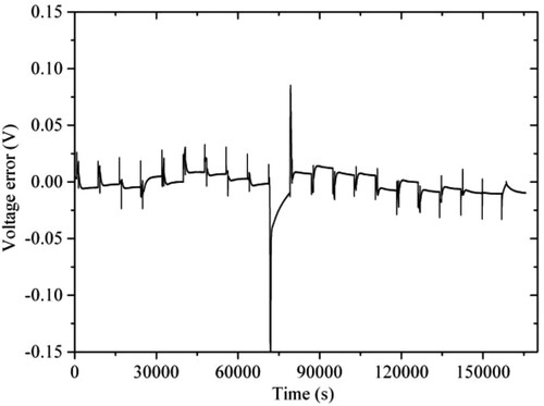
To validate the accuracy of parameter identification, the measured voltage and that from the model are compared, as shown in Figure 6, and the voltage error curve is shown in Figure 7. It can be observed that the predicted voltage from the model can match the measured voltage except for the stages of the end of the discharging HPPC test and the start of the charging HPPC test. The large voltage error is due to unstable dynamic characteristics of batteries under the condition of full discharging. For quantitative analysis, the mean absolute error (MAE) and RMSE of the predicted voltage are calculated, respectively, and the calculation results are also shown in Table 3. These results validate the parameter accuracy.

Figure 6. Comparison of the measured and model voltage under the HPPC test.

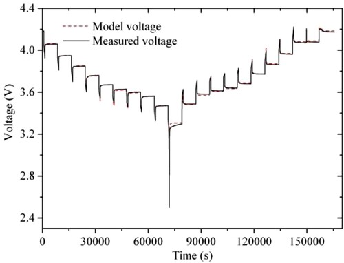
Figure 7. Voltage error between the measured and model voltage under the HPPC test.

4. BPNN-DEKF for the SOC estimation and online parameter identification

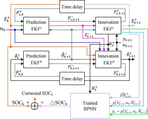
In general, the battery model parameters vary with working conditions, such as ambient temperature, the battery SOC, the discharging or charging current rate and battery ageing. To describe accurate behaviour inside batteries and improve SOC estimation accuracy, the model parameters should be identified online. In this paper, a dual extended Kalman filtering (DEKF) algorithm is proposed to estimate the battery SOC and update model parameters online. The first filter, $\text{EK}{\text{F}}^x$, predicts the battery SOC state,$x_k$, and the second filter, $\text{EK}{\text{F}}^{\theta }$, synchronously updates the model parameter state,${\theta }_k$. Meanwhile, a trained BP neural network is used for correcting the SOC estimation results from the first EKF filter.

A schematic of the proposed BPNN-DEKF algorithm is shown in Figure 8. Both filters exchange information with each other during iterative calculation and part information of the first estimator is used as the input of the trained BPNN.

Figure 8. Schematic of the proposed BPNN-DEKF algorithm.

4.1. Implementation of the first EKF

The implementation of the first EKF for predicting the battery SOC includes the following steps.

Step 1. Establish state and measurement equations: (11) $\begin{array}{rl}{x}_{k+1}& =f(x_k,u_k,{\theta }_k)+w_k^x\end{array}$(11) (12) $\begin{array}{rl}{y}_k& =g(x_k,u_k,{\theta }_k)+v_k^x\end{array}$(12) where $w_k^x$ and $v_k^x$ are the state and measurement noise, respectively. $w_k^x$ and $v_k^x$ are white noise and both mean values are zero. The variances of $w_k^x$ and $v_k^x$ are $Q_k^x$ and $R_k^x$, respectively.

Step 2. Predict state vector x: (13) ${\hat{x}}_{k+1}^{-}=f({\hat{x}}_k^{+},u_k,{\hat{\theta }}_{k+1}^{-})$(13) where ${\hat{\theta }}_{k+1}^{-}$ is the prediction of the vector $\theta$ from $\text{EK}{\text{F}}^{\theta }$ at the time of k+1.

Step 3. Predict the variance of estimate error: (14) $P_{x,k+1}^{-}=A({\hat{\theta }}_{k+1}^{-})P_{x,k}^{+}(A({\hat{\theta }}_{k+1}^{-}){)}^{\text{T}}+Q_k^x$(14)

Step 4. Calculate Kalman gain: (15) $K_k^x=P_{x,k+1}^{-}(H_k^x{)}^{\text{T}}(H_k^x{P}_{x,k+1}^{-}{(H_k^x)}^{\text{T}}+R_k^x{)}^{-1}$(15) where $H_k^x$ is the Jacobian matrix and can be expressed as (16) $\begin{array}{rl}{H}_k^x& ={\frac{\mathrm{\partial }g(\cdot )}{\mathrm{\partial }{x}_k}|}_{x_k={\hat{x}}_{k+1}^{-}}\\ & =\left[{\frac{\mathrm{\partial }OCV(SOC)}{\mathrm{\partial }SOC}|}_{SOC={\hat{x}}_{1,k+1}^{-}},-1,-1\right]\end{array}$(16)

Step 5. Update state vector x: (17) ${\hat{x}}_{k+1}^{+}={\hat{x}}_{k+1}^{-}+K_k^x(y_k-g({\hat{x}}_{k+1}^{-},u_k,{\hat{\theta }}_{k+1}^{-}))$(17)

Step 6. Update the variance of estimate error: (18) $P_{x,k+1}^{+}=(I-K_k^x{H}_k^x)P_{x,k+1}^{-}$(18) where $I$ denotes the unit matrix.

4.2. Implementation of the second EKF

Although the model parameters vary with the battery working conditions, they change slowly with time. Based on such a fact, the parameter vector ${\theta }_k$ is treated as constant and only superimposed by the noise. The implementation of the second EKF for the online updating parameter includes the following steps.

Step 1. Establish state and measurement equations: (19) $\begin{array}{rl}{\theta }_{k+1}& ={\theta }_k+w_k^{\theta }\end{array}$(19) (20) $\begin{array}{rl}{y}_k& =g(x_k,u_k,{\theta }_k)+v_k^{\theta }\end{array}$(20) where $w_k^{\theta }$ and $v_k^{\theta }$ are the state and measurement noise for the vector $\theta$, respectively. $w_k^{\theta }$ and $v_k^{\theta }$ are white noise and both mean values are zero. The variances of $w_k^{\theta }$ and $v_k^{\theta }$ are $Q_k^{\theta }$ and $R_k^{\theta }$, respectively.

Step 2. Predict state vector $\theta$: (21) ${\hat{\theta }}_{k+1}^{-}={\hat{\theta }}_k^{+}$(21)

Step 3. Predict the variance of estimate error: (22) $P_{\theta ,k+1}^{-}=P_{\theta ,k}^{+}+Q_k^{\theta }$(22)

Step 4. Calculate Kalman gain: (23) $K_k^{\theta }=P_{\theta ,k+1}^{-}(H_k^{\theta }{)}^{\text{T}}(H_k^{\theta }{P}_{\theta ,k+1}^{-}{(H_k^{\theta })}^{\text{T}}+R_k^{\theta }{)}^{-1}$(23)

Step 5. Update state vector $\theta$: (24) ${\hat{\theta }}_{k+1}^{+}={\hat{\theta }}_{k+1}^{-}+K_k^{\theta }(y_k-g({\hat{x}}_{k+1}^{-},u_k,{\hat{\theta }}_{k+1}^{-}))$(24)

Step 6. Update the variance of estimate error: (25) $P_{\theta ,k+1}^{+}=(I-K_k^{\theta }{H}_k^{\theta })P_{\theta ,k+1}^{-}$(25) where $H_k^{\theta }$ is also the Jacobian matrix and its calculation is quite complicated. Equations (8) and (9) are listed again to clearly show the calculation process. (26) $\begin{array}{rl}f(x_k,u_k,{\theta }_k)& =\left[\begin{array}{ccc}1& 0& 0\\ 0& 1-{\theta }_{3,k}& 0\\ 0& 0& 1-{\theta }_{5,k}\end{array}\right]x_k+\left[\begin{array}{c}-\frac{\eta T_S}{C_{\text{p}}}\\ {\theta }_{2,k}\\ {\theta }_{4,k}\end{array}\right]u_k\end{array}$(26) (27) $\begin{array}{rl}g(x_k,u_k,{\theta }_k)& =OCV(x_{1,k})-{\theta }_{1,k}{u}_k-x_{2,k}-x_{3,k}\end{array}$(27)

It should be noted that the sample time, $T_S$, is 1 s, and for simplicity, the charge–discharge efficiency $\eta$ is fixed as 1 in this paper. The calculation process $H_k^{\theta }$ is as follows. (28) $\begin{array}{rl}{H}_k^{\theta }& ={\frac{dg({\hat{x}}_{k+1}^{-},u_{k+1},{\theta }_k)}{d{\theta }_k}|}_{{\theta }_k={\hat{\theta }}_{k+1}^{-}}\end{array}$(28) (29) $\begin{array}{rl}\frac{dg({\hat{x}}_{k+1}^{-},u_{k+1},{\theta }_k)}{d{\theta }_k}& =\frac{\mathrm{\partial }g({\hat{x}}_{k+1}^{-},u_{k+1},{\theta }_k)}{\mathrm{\partial }{\theta }_k}\\ & +\frac{\mathrm{\partial }g({\hat{x}}_{k+1}^{-},u_{k+1},{\theta }_k)}{\mathrm{\partial }{\hat{x}}_{k+1}^{-}}\cdot \frac{d{\hat{x}}_{k+1}^{-}}{d{\theta }_k}\end{array}$(29) (30) $\begin{array}{rl}\frac{\mathrm{\partial }g({\hat{x}}_{k+1}^{-},u_{k+1},{\theta }_k)}{\mathrm{\partial }{\theta }_k}& =[-u_k,0,0,0,0]\end{array}$(30) (31) $\begin{array}{rl}\frac{\mathrm{\partial }g({\hat{x}}_{k+1}^{-},u_{k+1},{\theta }_k)}{\mathrm{\partial }{\hat{x}}_{k+1}^{-}}& =\left[{\frac{\mathrm{\partial }OCV(SOC)}{\mathrm{\partial }SOC}|}_{SOC={\hat{x}}_{1,k+1}^{-}},-1,-1\right].\end{array}$(31)

Next, we calculate $\frac{d{\hat{x}}_{k+1}^{-}}{d{\theta }_k}$ and define it as $D_k^{\theta }$. (32) $\begin{array}{rl}{D}_k^{\theta }& =\frac{d{\hat{x}}_{k+1}^{-}}{d{\theta }_k}=\frac{\mathrm{\partial }f({\hat{x}}_k^{+},u_k,{\theta }_k)}{\mathrm{\partial }{\theta }_k}+\frac{\mathrm{\partial }f({\hat{x}}_k^{+},u_k,{\theta }_k)}{\mathrm{\partial }{\hat{x}}_k^{+}}\cdot \frac{d{\hat{x}}_k^{+}}{d{\theta }_k}\end{array}$(32) (33) $\begin{array}{rl}\frac{\mathrm{\partial }f({\hat{x}}_k^{+},u_k,{\theta }_k)}{\mathrm{\partial }{\theta }_k}& =\left[\begin{array}{ccccc}0& 0& 0& 0& 0\\ 0& u_k& -{\hat{x}}_{2,k}^{+}& 0& 0\\ 0& 0& 0& u_k& -{\hat{x}}_{3,k}^{+}\end{array}\right]\end{array}$(33) (34) $\begin{array}{rl}\frac{\mathrm{\partial }f({\hat{x}}_k^{+},u_k,{\theta }_k)}{\mathrm{\partial }{\hat{x}}_k^{+}}& =\left[\begin{array}{ccc}1& 0& 0\\ 0& 1-{\hat{\theta }}_{3,k+1}^{-}& 0\\ 0& 0& 1-{\hat{\theta }}_{5,k+1}^{-}\end{array}\right]\end{array}$(34)

According to Equation (17), we can get (35) $\frac{d{\hat{x}}_k^{+}}{d{\theta }_k}=D_{k-1}^{\theta }-K_{k-1}^x{H}_{k-1}^{\theta }.$(35)

In Equation (35), both initial values of $D_k^{\theta }$ and $H_k^{\theta }$, namely $D_0^{\theta }$ and $H_0^{\theta }$, are zero. As a result, the value of $\frac{d{\hat{x}}_k^{+}}{d{\theta }_k}$, $D_k^{\theta }$ as well as $H_k^{\theta }$ can be obtained by recursive calculation using the above equations.

4.3. The BPNN for SOC estimation correction

Using any estimator to estimate the battery SOC will produce an estimation error. If the estimation error is known, the accurate SOC can be obtained by adding the estimation error to the SOC estimated by estimators. However, the SOC estimation error and the input/output variables of estimators are highly nonlinear, thus it is difficult to describe their relationship using a certain function. It is well known that the neural network has a powerful ability to address a nonlinear problem. In this paper, we use a back propagation neural network (BPNN) to predict the SOC estimation error. BPNN was first proposed by Rumelhart and McClelland in 1986. It is a multilayer feedforward neural network trained according to the error back-propagation algorithm, in other words, the signal forward propagates and the error back propagates in BPNN. Its basic idea is the gradient descent method, which uses the gradient search technique to minimise the RMSE between the actual and the expected output of the network. The basic BP algorithm includes two processes: signal forward-propagation and error back-propagation. That is, the error output is calculated in the direction from input to output, while the weight and threshold are adjusted in the direction from output to input. During forward propagation, the input signal acts on the output node through the hidden layer, and after nonlinear transformation, the output signal is generated. If the actual output is inconsistent with the expected output, it will turn into the back-propagation process of error. Error back-propagation is to transfer the output error layer by layer from the hidden layer to the input layer, and allocate the error to all units of each layer. The error signal obtained from each layer is used as the basis for adjusting the weight of each unit. By adjusting the connection weight between the input node and the hidden layer node, and the connection weight and threshold between the hidden layer node and the output node, the error decreases along the gradient direction. After repeated learning and training, the network parameters (weight and threshold) corresponding to the minimum error are determined, and the training is stopped. Considering the computational burden, the number of hidden layers of the used BPNN in this paper is limited to two. Figure 9 shows the structure of the BPNN with two hidden layers for SOC estimation correction.

Figure 9. Structure of the BPNN for correcting the SOC.

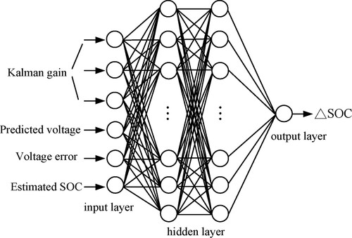
It can be seen from Figure 9 that the input layer has six neurons corresponding to six input variables, i.e. three elements in the Kalman gain vector of the first EKF, the predicted voltage, voltage error and the estimated SOC. The BPNN is designed for predicting the SOC estimation error, and hence an output layer has only one neuron. In addition, it has two hidden layers, and each hidden layer has a number of neurons. The output layer obtains the SOC estimation error using the information from the hidden layers with the action of the activation function. Before using the BPNN to predict SOC estimation error, we need to train it to obtain appropriate connection weight and threshold.

5. Results and discussion

To validate the effectiveness of the proposed method, the DST, BJDST, FUDSand US06 tests were respectively conducted for the SOC estimation. Considering the influence of over-charging and over-discharging on battery life and safety, the battery was operated at the level of 10%−80% SOC during all the tests. To validate the superiority of online parameter identification as well as BPNN for SOC correction, SOC estimation comparisons between the methods with and without BPNN correction as well as online parameter identification are implemented.

5.1. SOC estimation results without BPNN correction

In Section 3.3, the battery model parameters have been offline obtained under the discharging and charging HPPC tests. However, the AGA-based obtained model parameters may not be suitable for the battery model under the DST, BJDST, FUDS or US06 test. To clarify this question, we use a single EKF (recorded as EKF) and the proposed DEKF to estimate the battery SOC without BPNN correction, respectively, furthermore compare their results. It should be noted that both the EKF and DEFK use the second-order RC circuit model. The difference between them is that the model parameters in Table 3 are used and unchanged during the SOC estimation for the EKF, while the model parameters are updated online for the DEKF. The model parameters in Table 3 are only used as initial parameters to find the real parameter as soon as possible when the DEKF works. We regard the calculated SOC based on the CC method as the reference SOC. The initial SOC is set as real value, namely, 80%.

Figure 10(a) shows the comparisons of the battery SOC estimation between the DEKF and EKF under the DST test. It is obvious that the DEKF-based estimated SOC can track the reference SOC well, while the EKF-based estimated SOC deviates from the reference SOC after 3000 s. Figure 10(b) shows the comparisons of the SOC estimation errors. It can be observed that the SOC estimation error of the DEKF is much less than that of the EKF. The SOC maximum absolute error for the EKF reaches 10%, while only 3% for the DEKF. The calculated SOC MAEs and RMSEs for the DEKF and EKF are 1.19% and 1.26%, and 4.55% and 5.62%, respectively. Figure 10(c) shows the comparisons of the model voltage predicted by the DEKF and EKF under the DST test. It can be observed that the DEKF-based predicted model voltage and the measured voltage are almost identical. However, obviously, the EKF-based predicted model voltage far exceeds the measured voltage. The comparisons of prediction voltage error between the DEKF and EKF are shown in Figure 10(d). The voltage maximum absolute error for the EKF reaches 200 mV, while only less than 50 mV for the DEKF. The calculated voltage RMSEs and MAEs for the DEKF and EKF are 12.6 and 8.2, and 46.3 and 26.6 mV, respectively. The EKF-based estimated SOC and predicted model voltage indicate that there will lead to a large SOC error if offline-identified parameters are used to predict the model voltage. This is because the test conditions have changed, resulting in offline-identified parameters are not applicable, while DEKF addresses the problem by updating the model parameters online during the estimation process. It should be noted that the model voltage prediction error peaks at the time when the discharging current decreases or increases suddenly, which is owing to the battery polarisation effect. The result of the effect is the battery model parameters will change if a sharply varying current excites the battery, resulting in a large SOC estimation error. Nevertheless, the DEKF-based SOC error keeps still a small value because the model parameters are online updated.

Figure 10. Result comparisons under the DST test: (a) the estimated SOC; (b) SOC errors; (c) the predicted voltage; (d) voltage errors.

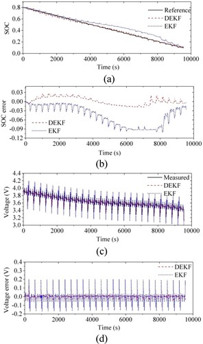
Figures 11–13 show the result comparisons between the DEKF and EKF under the BJDST, FUDS and US06 tests, respectively. Similar results to those obtained under the DST test, the DEKF-based SOC and voltage errors under the three tests are much less than those based on the EKF. The results demonstrate the superiority of the DEKF to the EKF; on the contrary, the EKF performs poorly both in SOC estimation and voltage prediction. For the SOC estimation using EKF, the battery model parameters are fixed. The model parameters are identified by the AGA algorithm under the HPPC test. Although parameter identification results in the whole SOC value are satisfactory, the possibility of inaccurate identification within a certain range of SOC is not excluded. This is a possible reason that the estimated SOC with EKF always suffers from a large error during about 4000–8000 s in Figures 10–13. The calculated SOC and voltage RMSEs/MAEs for the DEKF and EKF under all the tests are shown in Table 4, as these results indicate that the model parameters determined under a certain test are not suitable for the application of SOC estimation under other tests unless the model parameters are updated online or the estimated SOC is corrected.

Figure 11. Result comparisons under the BJDST test: (a) the estimated SOC; (b) SOC errors; (c) the predicted voltage; (d) voltage errors.

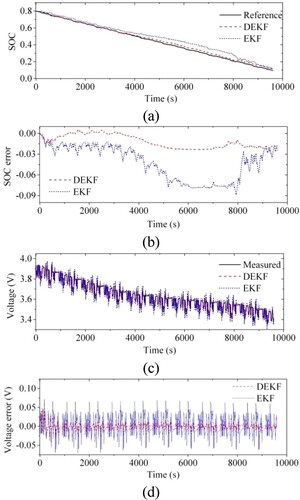
Figure 12. Result comparisons under the FUDS test: (a) the estimated SOC; (b) SOC errors; (c) the predicted voltage; (d) voltage errors.

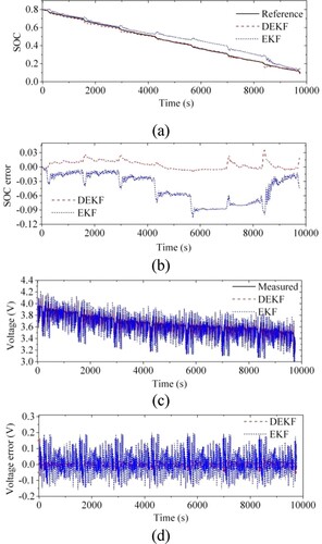
Figure 13. Result comparisons under the US06 test: (a) the estimated SOC; (b) SOC errors; (c) the predicted voltage; (d) voltage errors.

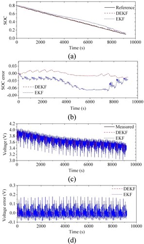
Table 4. SOC and voltage estimation errors without SOC correction under the DST, BJDST, FUDS and US06 tests.

		SOC error (%)		Voltage error (mV)
Method	Test profile	RMSE	MAE	RMSE	MAE
EKF	DST	5.62	4.55	46.3	26.6
	BJDST	4.90	4.24	23.6	19.6
	FUDS	5.27	4.36	51.7	37.7
	US06	4.44	3.97	40.1	30.8
DEKF	DST	1.26	1.09	12.6	8.2
	BJDST	1.51	1.25	7.0	4.6
	FUDS	0.98	0.79	11.7	8.6
	US06	0.97	0.86	7.4	4.9

5.2. Training and testing of BPNN

As described in Section 4.3, the proposed method uses BPNN to predict the SOC estimation error in real-time and then further correct the battery SOC. We need to train the BPNN before using it. Training BPNN is essentially a process of continual readjustment between the connection weights and the threshold, in order to make the BPNN error decrease to a preset minimum or stop at a preset training step. Then input the forecasting samples to the trained BPNN and obtain the forecasting results.

The training samples are from the above SOC estimation results under the DST, BJDST, FUDS and US06 tests. There produce 38,110 samples in the process of the SOC estimation using the DEKF, including 9550 samples under the DST test, 9600 samples under the BJDST test, 9760 samples under the FUDS test and 9200 samples under the US06 test. Similarly, there produce such 38,110 samples when using the EKF to estimate the SOC. The DEKF and EKF with SOC correction use their own samples to train their own BPNN. 38,110 samples are divided into two groups, one for training the BPNN and the other for testing the BPNN. The number of training samples accounts for 80% of the total. Test samples are evenly drawn from the total samples, as they cover the SOC ranging from 0.1 to 0.8. In other words, training samples consist of 7640 DST samples, 7680 BJDST samples, 7808 FUDS samples and 7360 US06 samples. For example, the formation process of 7360 US06 samples covering the SOC ranging from 0.1 to 0.8 is given as follows. In the SOC range of 0.1 to –0.8, 9200 US06 samples are divided into 1840 groups according to 5 discrete data points in each group. We select the first 4 data points of each group as training data and the last as test data. As described in Section IV (C), the input layer of the BPNN has 6 neurons, namely, the dimension of input of the BPNN is 6. Considering the large difference of amplitude between each dimension, for example, the predicted voltage is V-level, while the voltage error is only mV-level, the input of samples is normalised for improving the training speed and generalisation ability of the network. In this paper, the input of samples is normalised according to Equation (36). (36) $i{n}_{n,k}=\frac{(i{n}_k-i{n}_{min})}{(i{n}_{max}-i{n}_{min})}$(36) where $i{n}_k$ is the k-th variable to be normalised, $i{n}_{max}$ and $i{n}_{min}$ are the maximum and minimum of input sequences, respectively, and $i{n}_{n,k}$ is the result after normalisation. Obviously, $i{n}_k$ is converted into a value between 0 and 1. No normalisation is applied to the output of samples because it is a dimension variable.

In order to find a perfect BPNN, we construct single-hidden-layer-based and double-hidden-layer-based BPNNs. Each hidden layer has 1–30 neurons, and in addition, we specify that two hidden layers in double-hidden-layer-based BPNN have the same number of neurons. Therefore, both single-hidden-layer-based and double-hidden-layer-based BPNNs have 30 different network structures. The reason why the maximum number of hidden layers and the maximum number of neurons in each hidden layer is selected as 2 and 30, respectively, is based on the consideration of the real-time requirements of the SOC estimation. We use identical samples to train these BPNNs. Figure 14 shows the comparisons of training mean squared error (MSE) between these BPNNs. It can be observed that the MSEs of the double-hidden-layer BPNNs are less than those of the single-hidden-layer BPNNs with the same number of neurons as double-hidden-layer BPNNs. This indicates that the double-hidden-layer BPNN has more ability to predict the SOC estimation error than the single-hidden-layer BPNN. We also design a number of three-hidden-layer BPNNs. However, their performance has hardly improved compared with double-hidden-layer BPNNs, which indicates that using a double-hidden-layer BPNN is sufficient for predicting the SOC estimation error. The use of more complicated BPNNs cannot improve the performance for predicting the SOC estimation error but will increase the computational cost.

Figure 14. Comparisons of training mean squared error (MSE) between a series of single and double hidden layer BPNNs. The number of neurons in the hidden layer is from 1 to 30.

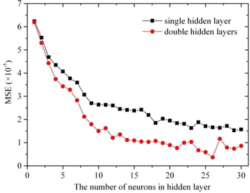
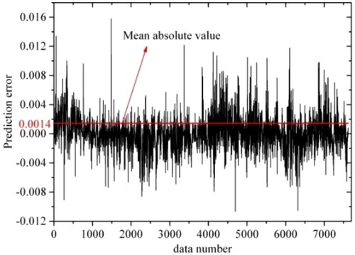
It can be seen from Figure 14 that the MSE reaches the smallest when the double-hidden-layer BPNN has 26 neurons in each hidden layer. Therefore, in this paper, we finally use this BPNN to predict estimation error in the process of SOC estimation. To further evaluate its performance, the BPNN is tested through test samples. The test results are shown in Figure 15. It can be observed that the SOC estimation error predicted by the BPNN can meet well with the real error, and even there is good consistency at the peak of the error. Figure 16 shows the error of the SOC estimation error predicted by the BPNN through test samples. Most of the errors are located between – 0.004 and +0.004. The red line in the figure is the mean absolute value of the errors and only 0.0014. These results indicate that the BPNN has been trained well and has good performance for predicting the SOC estimation error.

Figure 15. The test results of the BPNN for test samples.

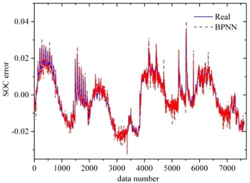
Figure 16. The error of the SOC estimation error predicted by the BPNN for test samples.

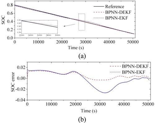
5.3. SOC estimation results with correction by BPNN

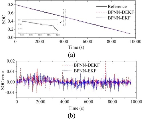
The trained BPNN can be used to predict the SOC estimation error in real-time. The SOC estimated by DEKF/EKF estimators is corrected by adding the predicted estimation error to obtain accurate SOC. Figure 17(a) shows the SOC estimation results with correction by the BPNN under the DST test. It can be observed that the corrected SOC can match well with the reference for the DEKF or EKF method. When no SOC correction is implemented, there is a large difference in the accuracy of SOC estimation between the DEKF and EKF methods. However, such a difference has been eliminated using the BPNN to correct the SOC. Figure 17(b) shows the SOC estimation errors. It can be observed that the SOC errors reduce considerably compared with the case of no correction. The RMSE and MAE for the DEKF reduce from 1.26% and 1.09% to 0.18% and 0.13%, respectively, while the EKF reduced from 5.62% and 4.55% to 0.21% and 0.14%, respectively.

Figure 17. SOC estimation results with correction by BPNN under the DST test: (a) the estimated SOC; (b) SOC errors.

Figures 18–20 show the SOC estimation results with correction by the BPNN under the BJDST, FUDS and US06 tests, respectively. From these figures, we can get results similar to those obtained under the DST test. All corrected SOC under the three dynamic tests can match well with the reference whether for the DEKF or EKF method. Most of the SOC errors after correction are limited between – 0.5% and +0.5%. The calculated MAEs and RMSEs of the SOC estimation for the DEKF and EKF under all the tests are shown in Table 5. For the DEKF method, the SOC RMSE/MAE under all the tests reduces by an average of seven times compared with the case of no correction, while reduces by an average of thirty times for the EKF method. The satisfactory results further demonstrate the effectiveness and accuracy of the SOC correction by the BPNN.

Figure 18. SOC estimation results with correction by BPNN under the BJDST test: (a) the estimated SOC; (b) SOC errors.

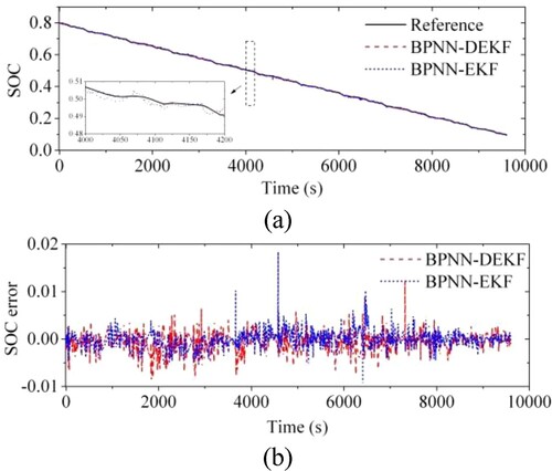
Figure 19. SOC estimation results with correction by BPNN under the FUDS test: (a) the estimated SOC; (b) SOC errors.

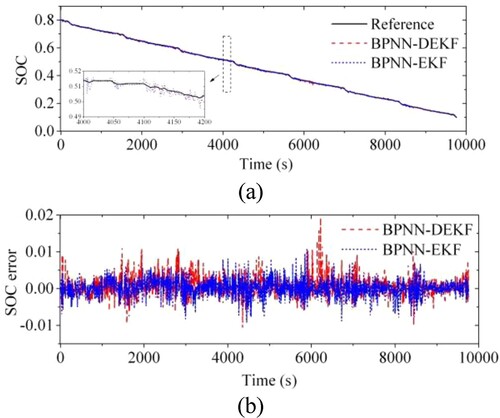
Figure 20. SOC estimation results with correction by BPNN under the US06 test: (a) the estimated SOC; (b) SOC errors.

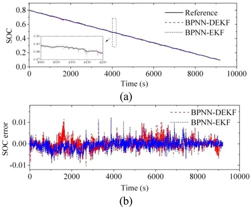
Table 5. SOC estimation errors with SOC correction by BPNN under the DST, BJDST, FUDS and US06 tests.

		SOC error (%)
Method	Test profile	RMSE	MAE
BPNN-EKF	DST	0.21	0.14
	BJDST	0.16	0.11
	FUDS	0.18	0.13
	US06	0.19	0.14
BPNN-DEKF	DST	0.18	0.13
	BJDST	0.18	0.13
	FUDS	0.21	0.15
	US06	0.22	0.16

To verify the generality of the proposed method, we conduct the SOC estimation under constant current conditions. The battery was discharged with a constant current of 0.1 A, while the trained BPNN is used to predict the SOC estimation error under constant current conditions. It should be noted that the BPNN was trained and tested under different working conditions at this time; that is, the training data-set excludes the data under constant current conditions. Figure 21(a) shows the SOC estimation results with correction by the BPNN under constant current conditions, and we can observe that the corrected SOC can match well with the reference for the DEKF or EKF method. The SOC estimation errors are shown in Figure 21(b) and can be observed that the SOC error of BPNN-DEKF is less than that of BPNN-EKF. The RMSE and MAE for the BPNN-DEKF and BPNN-EKF are 0.78% and 0.64%, and 1.32% and 1.12%, respectively. Compared with BPNN-EKF, BPNN-DEKF has minor SOC errors, demonstrating that BPNN-DEKF has stronger generality.

Figure 21. SOC estimation results with correction by BPNN under the constant current condition: (a) the estimated SOC; (b) SOC errors.

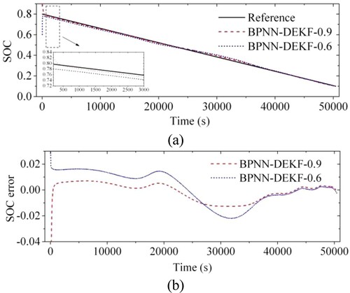
To further validate the robustness of the proposed method and examine the convergence performance of the algorithm, $SO{C}_0$ is set to an arbitrary incorrect value, say $SO{C}_0$ = 0.9 or 0.6. The SOC estimation curves are shown in Figure 22(a), and the estimation error curves are displayed in Figure 22(b). The estimated SOC can quickly track the reference value whether the initial SOC is 0.9 or 0.6. The RMSE and MAE using BPNN-DEKF to estimate SOC with the initial SOC of 0.9 and 0.6 are 0.86% and 0.72%, and 1.26% and 1.05%, respectively. The satisfactory results further demonstrate the effectiveness and robustness of the proposed method.

Figure 22. SOC estimation results with correction by BPNN under the constant current condition with wrong initial SOC value: (a) the estimated SOC; (b) SOC errors.

5.4. Comparisons with other methods

Table 6 compares the proposed BPNN-DEKF's estimation performance to other pure data-driven and model-based algorithms mentioned in the literature. These comparisons were conducted under similar or the same condition as this study.

Table 6. Comparisons of SOC estimation error by the latest pure data-driven and model-based estimation methods.

Ref.	Method	RMSE (%)	MAE (%)	Test profile
Xiao et al. (2021)	GRU-GPR	–	0.68	US06
Ma et al. (2021)	LSTM-DNN	0.82	0.63	UDDS
Tian et al. (2021)	DNN-KF	0.39	–	CCCV
Kim et al. (2021)	Nonlinear observer	–	0.70	UDDS
Liu et al. (2022)	FOAEKF-UKF	–	0.96	DST
He et al. (2021)	AIEKF	0.24	0.20	DST
Ours	BPNN-DEKF	0.18	0.13	DST
Ours	BPNN-DEKF	0.22	0.16	US06

5.5. Computational cost of the proposed method

Low computational cost is very important for real-time application. We write the codes about the proposed algorithm in MATLAB R2018a. The codes are executed on a system with Intel(R) Core(TM) i7-6600U CPU @ 2.6 GHz and 20 GB of RAM. The average code execution time is about 91 s for 9550 sample points.

6. Conclusion

In this paper, we employ a second-order RC circuit to model the battery and using the model a DEKF algorithm combined with a BPNN is proposed for the estimation and correction of the battery SOC. The DEKF is used to estimate the SOC and update the model parameters online, while the BPNN is used to correct the estimated SOC to further reduce the estimation error. The effectiveness and accuracy of the proposed method are demonstrated under four sophisticated dynamic tests, i.e. the DST, BJDST, FUDS and US06 tests. SOC estimation comparisons between the original DEKF and BPNN-based corrected DEKF methods show that the estimation error decreases considerably after correcting the estimated SOC. The corrected SOC RMSE/MAE under all four tests decreases by an average of seven times compared with the case of no correction. In addition, to further validate the superiority of online parameter identification and the performance of the SOC correction under the condition of large SOC error for example estimated by an ordinary method, comparisons of the SOC estimation between the DEKF and a single EKF with and without SOC correction are implemented. The results show that (1) there is a large difference in the accuracy of SOC estimation between the DEKF and EKF methods under the condition of no SOC correction. The SOC estimation accuracy of the EKF is only about a quarter of the DEKF, which indicates that online parameter identification improves the accuracy of the battery model and thus enhances the accuracy of the SOC estimation; (2) Such a large difference in the accuracy of SOC estimation between the DEKF and EKF methods can be eliminated if we use the BPNN to correct the estimated SOC. The SOC errors of both methods reduce considerably, and by an average of seven and thirty times, respectively. The results for the EKF method further verify the effectiveness and accuracy of the SOC correction by the BPNN. The generality and robustness of the proposed method are also verified by constant current discharge test.

Although satisfactory SOC estimation accuracy has been achieved in this paper, the effectiveness of the proposed method is demonstrated under only four dynamic tests. We will focus on the validation under more working conditions as well as the impact of temperature in future.

Disclosure statement

No potential conflict of interest was reported by the author(s).

Additional information

Funding

This work was supported by the project of the Natural Science Foundation of the Higher Education Institute of Anhui Province [grant number KJ2019A0106], and the Academic Support Project for Top-notch Talents in Disciplines (Majors) of Colleges and Universities in Anhui Province [grant number gxbjZD2021052].

References

- Adaikkappan, M., & Sathiyamoorthy, N. (2022). Modeling, state of charge estimation, and charging of lithium-ion battery in electric vehicle: A review. International Journal of Energy Research, 46(3), 2141–2165. https://doi.org/10.1002/er.7339
- An, F., Jiang, J., Zhang, W., Zhang, C., & Fan, X. (2022). State of energy estimation for lithium-ion battery pack via prediction in electric vehicle applications. IEEE Transactions on Vehicular Technology, 71(1), 184–195. https://doi.org/10.1109/TVT.2021.3125194
- Chen, H., Yu, Y., Jia, Y., & Zhang, L. (2022). Safe transductive support vector machine. Connection Science, 34(1), 942–959. https://doi.org/10.1080/09540091.2021.2024511
- Duan, W., Song, C., Chen, Y., Xiao, F., Peng, S., Shao, Y., & Song, S. (2020). Online parameter identification and state of charge estimation of battery based on multitimescale adaptive double Kalman filter algorithm. Mathematical Problems in Engineering, 2020(12), Article 9502605. https://doi.org/10.1155/2020/9502605
- Ephrem, C., Kollmeyer, P. J., Matthias, P., & Ali, E. (2018). State-of-charge estimation of Li-ion batteries using deep neural networks: A machine learning approach. Journal of Power Sources, 400(8), 242–255. https://doi.org/10.1016/j.jpowsour.2018.06.104
- Ezemobi, E., Silvagni, M., Mozaffari, A., Tonoli, A., & Khajepour, A. (2022). State of health estimation of lithium-ion batteries in electric vehicles under dynamic load conditions. Energies, 15(3), 1234. https://doi.org/10.3390/en15031234
- Guo, F., Hu, G., Xiang, S., Zhou, P., Hong, R., & Xiong, N. (2019). A multi-scale parameter adaptive method for state of charge and parameter estimation of lithium-ion batteries using dual Kalman filters. Energy, 178(7), 79–88. https://doi.org/10.1016/j.energy.2019.04.126
- Guo, X., Kang, L., Yao, Y., Huang, Z., & Li, W. (2016). Joint estimation of the electric vehicle power battery state of charge based on the least squares method and the Kalman filter algorithm. Energies, 9(2), 100. https://doi.org/10.3390/en9020100
- He, W., Williard, N., Chen, C., & Pecht, M. (2013). State of charge estimation for electric vehicle batteries using unscented Kalman filtering. Microelectronics Reliability, 53(6), 840–847. https://doi.org/10.1016/j.microrel.2012.11.010
- He, Z., Li, Y., Sun, Y., Zhao, C., Lin, C., Pan, C., & Wang, L. (2021). State-of-charge estimation of lithium ion batteries based on adaptive iterative extended Kalman filter. Journal of Energy Storage, 39(7), Article 102593. https://doi.org/10.1016/j.est.2021.102593
- Hu, C., Ma, L., Guo, S., & Han, Z. (2022). Deep learning enabled state-of-charge estimation of LiFePO4 batteries: A systematic validation on state-of-the-art charging protocols. Energy, 246(5), Article 123404. https://doi.org/10.1016/j.energy.2022.123404
- Hu, X., Yuan, H., Zou, C., Li, Z., & Zhang, L. (2018). Co-estimation of state of charge and state of health for lithium-ion batteries based on fractional-order calculus. IEEE Transactions on Vehicular Technology, 67(11), 10319–10329. https://doi.org/10.1109/TVT.2018.2865664
- Ibrahim, A., & Jiang, F. (2021). The electric vehicle energy management: An overview of the energy system and related modeling and simulation. Renewable and Sustainable Energy Reviews, 144(7), Article 111049. https://doi.org/10.1016/j.rser.2021.111049
- Jwa, B., Dan, Z. B., & Cz, A. (2020). An overview of electricity powered vehicles: Lithium-ion battery energy storage density and energy conversion efficiency. Renewable Energy, 162(12), 1629–1648. https://doi.org/10.1016/j.renene.2020.09.055
- Kim, D., Goh, T., Park, M., & Kim, S. W. (2015). Fuzzy sliding mode observer with grey prediction for the estimation of the state-of-charge of a lithium-ion battery. Energies, 8(11), 12409–12428. https://doi.org/10.3390/en81112327
- Kim, W. Y., Lee, P. Y., Kim, J., & Kim, K. S. (2021). A robust state of charge estimation approach based on nonlinear battery cell model for lithium-ion batteries in electric vehicles. IEEE Transactions on Vehicular Technology, 70(6), 5638–5647. https://doi.org/10.1109/TVT.2021.3079934
- Ling, L., & Wei, Y. (2021). State-of-charge and state-of-health estimation for lithium-ion batteries based on dual fractional-order extended Kalman filter and online parameter identification. IEEE Access, 9(3), 47588–47602. https://doi.org/10.1109/ACCESS.2021.3068813
- Liu, W., Zhou, H., Tang, Z., & Wang, T. (2022). State of charge estimation algorithm based on fractional-order adaptive extended Kalman filter and unscented Kalman filter. ASME Journal of Electrochemical Energy Conversion and Storage, 9(2), 021005. https://doi.org/10.1115/1.4051941
- Lv, J., Jiang, B., Wang, X., Liu, Y., & Fu, Y. (2020). Estimation of the state of charge of lithium batteries based on adaptive unscented Kalman filter algorithm. Electronics, 9(9), 1425. https://doi.org/10.3390/ELECTRONICS9091425
- Ma, L., Hu, C., & Cheng, F. (2021). State of charge and state of energy estimation for lithium-ion batteries based on a long short-term memory neural network. The Journal of Energy Storage, 37, Article 102440. https://doi.org/10.1016/j.est.2021.102440
- Mao, X., Song, S., & Ding, F. (2022). Optimal BP neural network algorithm for state of charge estimation of lithium-ion battery using PSO with levy flight. The Journal of Energy Storage, 49(2), Article 104139. https://doi.org/10.1016/j.est.2022.104139
- Ming, C., Weijie, C., & Xiaojun, T. (2017). Battery state-of-charge estimation based on a dual unscented kalman filter and fractional variable-order model. Energies, 10(10), 1577. https://doi.org/10.3390/en10101577
- Pavkovic, D., Krznar, M., Komljenovic, A., Hrgetic, M., & Zorc, D. (2017). Dual EKF-based state and parameter estimator for a LiFePO4 battery cell. Journal of Power Electronics, 17(2), 398–410. https://doi.org/10.6113/jpe.2017.17.2.398
- Peng, N., Zhang, S., & Zhang, X. (2021). Co-estimation for capacity and state of charge for lithium-ion batteries using improved adaptive extended kalman filter. The Journal of Energy Storage, 40(8), Article 102559. https://doi.org/10.1016/j.est.2021.102559
- Qays, M. O., Buswig, Y., Hossain, M. L., & Abu-Siada, A. (2022). Recent progress and future trends on the state of charge estimation methods to improve battery-storage efficiency: A review. CSEE Journal of Power and Energy Systems, 8(1), 105–114. https://doi.org/10.17775/CSEEJPES.2019.03060
- Qiao, Z., Liang, L., Hu, X., Xiong, N., & Hu, G. (2017). H∞-based nonlinear observer design for state of charge estimation of lithium-ion battery with polynomial parameters. IEEE Transactions on Vehicular Technology, 99, 1–13. https://doi.org/10.1109/TVT.2017.2723522
- She, C., Zhang, L., Wang, Z., Sun, F., Liu, P., & Song, C. (2021). Battery state of health estimation based on incremental capacity analysis method: Synthesizing from cell-level test to real-world application. IEEE Journal of Emerging and Selected Topics in Power Electronics. https://doi.org/10.1109/JESTPE.2021.3112754.
- Shrivastava, P., Soon, T. K., Idris, M., & Mekhilef, S. (2019). Overview of model-based online state-of-charge estimation using kalman filter family for lithium-ion batteries. Renewable and Sustainable Energy Reviews, 113(10), 109233. https://doi.org/10.1016/j.rser.2019.06.040
- Su, L., Zhou, G., Hu, D., Liu, Y., & Zhu, Y. (2021). Research on the state of charge of lithium-ion battery based on the fractional order model. Energies, 14(19), 6307. https://doi.org/10.3390/en14196307
- Sun, D., Yu, X., Wang, C., Zhang, C., & Bhagat, R. (2020). State of charge estimation for lithium-ion battery based on an intelligent adaptive extended kalman filter with improved noise estimator. Energy, 214(1), Article 119025. https://doi.org/10.1016/j.energy.2020.119025
- Sun, X., Wang, Q., Zhang, X., Xu, C., & Zhang, W. (2022). Deep blur detection network with boundary-aware multi-scale features. Connection Science, 34(1), 766–784. https://doi.org/10.1080/09540091.2021.1933906
- Tian, J., Xiong, R., Shen, W., & Lu, J. (2021). State-of-charge estimation of lifepo4 batteries in electric vehicles: A deep-learning enabled approach. Applied Energy, 291(3), Article 116812. https://doi.org/10.1016/j.apenergy.2021.116812
- Wang, Q., Ye, M., Wei, M., Lian, G., & Wu, C. (2021). Co-estimation of state of charge and capacity for lithium-ion battery based on recurrent neural network and support vector machine. Energy Reports, 7(11), 7323–7332. https://doi.org/10.1016/j.egyr.2021.10.095
- Wang, S., Tu, C., & Juang, J. (2022). Automatic traffic modelling for creating digital twins to facilitate autonomous vehicle development. Connection Science, 34(1), 1018–1037. https://doi.org/10.1080/09540091.2021.1997914
- Wang, Y., & Chen, Z. (2020). A framework for state-of-charge and remaining discharge time prediction using unscented particle filter. Applied Energy, 260(C), Article 114324. https://doi.org/10.1016/j.apenergy.2019.114324
- Wang, Y., Tian, J., Sun, Z., Wang, L., & Chen, Z. (2020). A comprehensive review of battery modeling and state estimation approaches for advanced battery management systems. Renewable & Sustainable Energy Reviews, 131(C), Article 110015. https://doi.org/10.1016/j.rser.2020.110015
- Wang, Y., Xu, R., Zhou, C., Kang, X., & Chen, Z. (2022). Digital twin and cloud-side-end collaboration for intelligent battery management system. Journal of Manufacturing Systems, 62(11), 124–134. https://doi.org/10.1016/j.jmsy.2021.11.006
- Wang, Z., Song, C., Zhang, L., Zhao, Y., Liu, P., & Dorrell, D. G. (2021). A data-driven method for battery charging capacity abnormality diagnosis in electric vehicle applications. IEEE Transactions on Transportation Electrification, 8(1), 990–999. https://doi.org/10.1109/TTE.2021.3117841
- Xiao, F., Li, C., Fan, Y., Yang, G., & Tang, X. (2021). State of charge estimation for lithium-ion battery based on Gaussian process regression with deep recurrent kernel. International Journal of Electrical Power & Energy Systems, 124(7), Article 106369. https://doi.org/10.1016/j.ijepes.2020.106369
- Xiao, R., Shen, J., Li, X., Yan, W., Pan, E., & Chen, Z. (2016). Comparisons of modeling and state of charge estimation for lithium-ion battery based on fractional order and integral order methods. Energies, 9(3), 184. https://doi.org/10.3390/en9030184
- Xing, L., Ling, L., Gong, B., & Zhang, M. (2022). State-of-charge estimation for lithium-ion batteries using Kalman filters based on fractional-order models. Connection Science, 34(1), 162–184. https://doi.org/10.1080/09540091.2021.1978930
- Xiong, R., Cao, J., Yu, Q., He, H., & Sun, F. (2017). Critical review on the battery state of charge estimation methods for electric vehicles. IEEE Access, 6(2), 1832–1843. https://doi.org/10.1109/ACCESS.2017.2780258
- Xiong, R., He, H., Sun, F., & Zhao, K. (2013). Evaluation on state of charge estimation of batteries with adaptive extended kalman filter by experiment approach. IEEE Transactions on Vehicular Technology, 62(1), 108–117. https://doi.org/10.1109/TVT.2012.2222684
- Zhang, L., Hu, X., Wang, Z., Ruan, J., Ma, C., Song, Z., Dorrell, D. G., & Pecht, M. G. (2021). Hybrid electrochemical energy storage systems: An overview for smart grid and electrified vehicle applications. Renewable and Sustainable Energy Reviews, 139(4), Article 110581. https://doi.org/10.1016/j.rser.2020.110581
- Zhang, S., Guo, X., & Zhang, X. (2020). An improved adaptive unscented kalman filtering for state of charge online estimation of lithium-ion battery. The Journal of Energy Storage, 32(12), Article 101980. https://doi.org/10.1016/j.est.2020.101980
- Zhang, W., Wang, L., Wang, L., Liao, C., & Zhang, Y. (2022). Joint state-of-charge and state-of-available-power estimation based on the online parameter identification of lithium-ion battery model. IEEE Transactions on Industrial Electronics, 69(4), 3677–3688. https://doi.org/10.1109/TIE.2021.3073359
- Zheng, C., Fu, Y., & Mi, C. C. (2013). State of charge estimation of lithium-ion batteries in electric drive vehicles using extended kalman filtering. IEEE Transactions on Vehicular Technology, 62(3), 1020–1030. https://doi.org/10.1109/TVT.2012.2235474
- Zheng, F., Xing, Y., Jiang, J., Sun, B., Kim, J., & Pecht, M. (2016). Influence of different open circuit voltage tests on state of charge online estimation for lithium-ion batteries. Applied Energy, 183(10), 513–525. https://doi.org/10.1016/j.apenergy.2016.09.010
- Zhu, Q., Xu, M., Liu, W., & Zheng, M. (2019). A state of charge estimation method for lithium-ion batteries based on fractional order adaptive extended kalman filter. Energy, 187(11), Article 115880. https://doi.org/10.1016/j.energy.2019.115880