Energy-efficient control of thermal comfort in multi-zone residential HVAC via reinforcement learning

Abstract

Energy efficient control of thermal comfort has been already an important part of residential heating, ventilation, and air conditioning (HVAC) systems. However, the optimisation of energy saving control for thermal comfort is not an easy task due to the complex dynamics of HVAC systems, the dynamics of thermal comfort and the trade-off between energy saving and thermal comfort. To solve the above problem, we propose a deep reinforcement learning-based thermal comfort control method in multi-zone residential HVAC. In this paper, firstly we design a SVR-DNN model, consisting of Support Vector Regression and a Deep Neural Network to predict thermal comfort value. Then, we apply Deep Deterministic Policy Gradient (DDPG) based on the output of the SVR-DNN model to achieve an optimal HVAC thermal comfort control strategy. This method can minimise energy consumption while satisfying occupants' thermal comfort. The experimental results show that our method can improve thermal comfort prediction performance by 20.5% compared with DNN; compared with deep Q-network (DQN), energy consumption and thermal comfort violation can be reduced by 3.52% and 64.37% respectively.

Keywords:

• Reinforcement learning
• deep reinforcement learning
• multi-zone residential HVAC
• energy consumption
• thermal comfort

1. Introduction

Building energy consumption accounts for about 40–50% of global energy consumption (Prez-Lombard et al., 2008) and 30% of all ${\mathrm{C}\mathrm{O}}_2$ emissions (Costa et al., 2013). The explosion of building density and urban population leads to an inevitable increase in building energy consumption. HVAC systems are the main method of indoor thermal comfort control and their proper regulation has a significant impact on occupants' satisfaction with thermal comfort. The energy consumption of the HVAC system is a significant proportion of the building energy consumption. Therefore, it is necessary to promote energy-comfort-related control strategies for smart building energy management (Moreno et al., 2017).

Currently, rule-based control(RBC) is widely adopted to solve control problems in HVAC systems, but they are based on engineers' experience and thus cannot learn knowledge from historical data to save energy effectively or satisfy occupants' thermal comfort requirements. Model predictive control(MPC) (Zeng & Barooah, 2020), a model-based control method, usually solves HVAC control problems better than RBC. However, MPC requires a large amount of historical data and real-time monitoring data to establish an accurate model to save energy while meeting occupants' thermal comfort requirements. In the single-zone HVAC control problem, a low-order model can be established for MPC to solve the control problem. However, in the multi-zone HVAC control problem, it is necessary to consider not only the indoor and outdoor heat exchange but also the heat exchange between zones, which makes the building thermal model more complex. It is difficult to establish an accurate model for MPC to solve the multi-zone HVAC control problem.

In order to overcome above problems, data-driven machine learning methods such as deep learning and reinforcement learning have received extensive attention and research. In Chen et al. (2022), researches involving machine learning have been developed to optimise industrial loads. Kheyrinataj and Nazemi (2020) propose a neural network algorithm to solve delay fractional optimal control problems. In Nazemi et al. (2019), a neural network framework-based method is proposed to solve the optimal control problem. In smart gird, Fatema et al. (2021) propose a deep learning based method to meeting grid requirements and Rocchetta et al. (2019) propose a RL framework to optimise power gird. In Qiu et al. (2020), a Q-learning based method is proposed to optimise HVAC systems to achieve energy savings during the cooling season. Nowadays, especially model-free optimal control methods based on deep reinforcement learning (DRL) Zhou et al. (2022) show good adaptability and robustness in control problems. In Han et al. (2019), a DRL method is used to optimise the energy management. Model-free control methods do not need to establish an accurate model to solve control problems.

There has also been some pioneering works utilising DRL to optimise HVAC system control. K. R. Kurte et al. (2021) use Deep Q-Network (DQN) to satisfy residential demand response and compared it to the model-based HVAC method. This work mainly focuses on the effect of temperature on thermal comfort. In addition, the method applied is only compared on discrete action space and not with methods that can handle continuous action space. Wei et al. (2021) use a DQN based approch for the HVAC control. Brandi et al. (2020) adopt the DRL method for indoor temperature control. All of the above research works have demonstrated the effectiveness of the DRL method for HVAC thermal control. However, the above studies solve optimal HVAC control on a discrete action space. Discrete spaces can limit the performance of thermal control. In Du et al. (2021) and Yu et al. (2019), the Deep Deterministic Policy Gradient(DDPG) method is used to achieve energy efficiency and comfort satisfaction without discretization. However, these research only focus on the effect of temperature on comfort and is more concerned with energy efficiency.

Motivated by the above concerns, we apply a method combining a thermal comfort prediction model and DRL to optimise residential multi-zone HVAC control. Our objective is to minimise energy consumption under the condition of satisfying occupants' thermal comfort requirements in HVAC systems. We evaluate RBC and three RL algorithms: Q-learning for discrete control, Deep Q-Network(DQN) for discrete action space control, Deep Deterministic Policy Gradient(DDPG) for continuous control in a multi-zone residential HVAC model, where Q-learning for traditional RL methods, DQN and DDPG for DRL methods. Our method also provides new ideas and techniques for maintaining a certain level of comfort in commercial and residential buildings while saving energy and reducing emissions. The main contributions of this paper aresummarised as follows:

1. We design a hybrid model based on Support Vector Regression (SVR) and a Deep Neural Network (DNN), called SVR-DNN, for predicting thermal comfort value which is taken as a part of the state and reward in reinforcement learning.

2. The multi-zone residential HVAC problem considering occupancy and heat exchange between zones is formulated as a reinforcement learning problem.

3. We apply Q-learning, DQN and DDPG methods to optimise HVAC control in a multi-zone residential HVAC model and compare the performance of these three algorithms. We show that these algorithms can reduce violation of thermal comfort compared with rule-based control in multi-zone HVAC control. Moreover, the DDPG method shows the best control performance.

4. We verify the adaptability of the method we propose under different regional weather conditions. And We also verify that the proposed method shows the best performance under different thermal comfort models.

The rest of the paper is organised as follows. The related work is described in Section 2. Section 3 introduces theoretical background of RL and DRL algorithms. The problem formulation of Multi-zone residential HVAC control is presented in Section 4. The simulation environment is introduced in Section 5. The simulation results are analysed in Section 6. Finally, Section 7 concludes the paper.

2. Related work

2.1. Thermal comfort

Thermal comfort is the level of satisfaction with the environment experienced by the occupants. Nowadays, a number of models have been developed to quantitatively evaluate thermal comfort. Shaw (1972) proposed the Predicted Mean Vote-Predicted Percentage Dissatisfied (PMV-PPD) model, which is based on a heat balance model. The model is designed to quantify the extent to which occupants perceive the environment as hot or cold. With the rapid development of ML, there have been a range of thermal comfort models based on ML algorithms. Zhou et al. (2020) used the support vector machine (SVM) algorithm to develop a thermal comfort model with self-learning and self-correction ability. In Liu et al. (2007), a model based on the Back Propagation(BP) neural network for individual thermal comfort was proposed.

2.2. Thermal comfort HVAC control

Baldi et al. (2018) proposed a switched self-tuning method to reduce energy and improve thermal comfort. Korkas et al. (2018) proposed an EMS strategy to change the energy demand considering the occupancy information. In Korkas et al. (2015), a distributed demand management system is proposed to be adaptable to different changes(weather or occupancy). The above study was carried out to obtain the control strategy by adaptive optimisation. In Wu et al. (2018), a hierarchical control strategy is used to provide primary frequency regulation in residential HVAC systems. Watari et al. (2021) adopted the MPC-based method for energy management and thermal comfort. Zeng and Barooah (2021) proposed an adaptive MPC scheme in HVAC systems for energy saving.

The above methods can all be classified as model-based methods, where the thermal dynamic environment of the HVAC needs to be modelled. However, the thermal environment influenced by a variety of factors that is difficult to be modelled precisely. model-free RL has been greatly developed in recent years, and as a result, many researchers have applied RL to deal with HVAC control problems. Qiu et al. (2020) implemented Q-learning and the model-based controller to respectively optimise building HVAC systems to save energy. In Brandi et al. (2020), deep reinforcement learning(DRL) is applied to optimise the problem of the supply water temperature setpoint in a heating system and the well-trained agent can save energy between 5% and 12%. Achieving energy savings from optimising HVAC control equates to cost savings. Jiang et al. (2021) proposed DQN with an action processor, saving close to 6% of total cost with demand charges, while close to 8% without demand charges. In Wei et al. (2021) applied a DRL-based algorithm for minimising the total energy cost while maintaining desired room temperature and meeting data centre workload deadline constraints. A deep Q-network (DQN) was applied to optimise four air-handling units (AHUs), two electric chillers, a cooling tower, and two pumps to minimise the energy consumption while maintaining the indoor ${\mathrm{C}\mathrm{O}}_2$ concentration (Ahn & Park, 2019). Zenger et al. (2013) implemented the RL algorithm to maintain thermal comfort while saving energy. In K. R. Kurte et al. (2021), authors implemented the DQN algorithm to achieve energy savings and meet comfort(temperature). Fu et al. (2022) proposed a distributed multi-agent DQN to optimise HVAC systems. Cicirelli et al. (2021) used DQN to balance energy consumption and thermal comfort. K. Kurte, Munk, Amasyali et al. (2020) and K. Kurte, Munk, Kotevska et al. (2020) applied DRL in residential HVAC control to save costs and maintain comfort. However, Q-learning and DQN can still only handle the discrete action space.

In Yu et al. (2019), a DRL method was applied for smart home energy management. Du et al. (2021) implemented the DDPG method to address the issue of 2-zone residential HVAC control strategies that allow for the lower bound of the user comfort level(temperature) with energy savings but they did not establish a thermal comfort prediction model. In McKee et al. (2020) and McKee et al. (2020) used DRL to optimise residential HVAC considering human occupancy to achieve energy savings. Sang and Sun (2021) applied DDPG to generate an HVAC cooling-heating-power strategy to solve the demand response problem. In Yu et al. (2021), a multi-agent DRL method is proposed in building HVAC control to minimise energy consumption. A concern with multi-agent algorithms is that as the number of zones increases, the number of neural networks increases, resulting in excessive computational costs. Based on these considerations, we propose a method combining DDPG and thermal comfort model for energy-efficient thermal comfort control in multi-zone residential HVAC. Our method is able to reduce energy consumption while meeting the thermal comfort requirements (Table 1).

Table 1. Review of thermal comfort in HVAC systems.

Method		Refs	Pros and Cons
Model-based	MPC, adaptive optimisation, hierarchical control	Baldi et al. (2018), Korkas et al. (2018, 2015), Wu et al. (2018), Watari et al. (2021), and Zeng and Barooah (2021)	The model-based method is able to learn strategies based on the system's own dynamic model and is more robust.However, the model-based method requires an accurate model and the dynamic model of the HVAC is difficult to build accurately.
	Q-learning, DQN, multi-agent DQN	Qiu et al. (2020), Brandi et al. (2020), Jiang et al. (2021), Wei et al. (2021), Ahn and Park (2019), Zenger et al. (2013), K. R. Kurte et al. (2021), Fu et al. (2022), Cicirelli et al. (2021), K. Kurte, Munk, Amasyali et al. (2020), and K. Kurte, Munk, Kotevska et al. (2020)	Q-learning, DQN and multi-agent DQN do not need to build accurate dynamic models to learn better strategies. However, they can only handle the discrete action space.
Model-free	DDPG	Yu et al. (2019), Du et al. (2021), McKee et al. (2020), and Sang and Sun (2021)	This literature applies DDPG (DDPG is able to handle continuous space and again does not require an accurate model) for optimal control to achieve energy savings and comfort requirements. However, they focus more on energy consumption and only on the temperature comfort.
	Multi-agent DDPG	Yu et al. (2021)	The literature uses a multi-agent DRL with attention mechanism to minimise energy consumption, assigning an agent to each zone to solve the high dimensional space problem. But the ensuing computational cost becomes high.

3. Theoretical background of algorithms

In this section, the theoretical background of RL and DRL is presented. And we concentrate on DDPG, DQN and Q-learning methods.

Reinforcement learning(RL) is a kind of trial and error learning through interaction with the environment (Montague, 1999). Its goal is to make the agent get the largest cumulative reward in the environmental interaction. The problem of reinforcement learning (RL) can be modelled as a Markov Decision Process (MDP), which includes a quintuple $〈\mathcal{S},\mathcal{A},r,p_1,\mathcal{P}〉$. MDP is shown in Figure 1.

1. $\mathcal{S}$ is the state space, $s_t\in \mathcal{S}$ indicates the state of the agent at time t.

2. $\mathcal{A}$ is the action space, $a_t\in \mathcal{A}$ represents the action taken by the agent at time t.

3. $r:\mathcal{S}\times \mathcal{A}\to \mathbb{R}$ is the reward function, $r_t\sim r(s_t,a_t)$ indicates the immediate reward value obtained by the agent executing the action $a_t$ in the state $s_t$.

4. $p_1$ is an initial state distribution with density $p_1\left(s_1\right)$.

5. $\mathcal{P}:\mathcal{S}\times \mathcal{S}\times \mathcal{A}\to [0,1]$ is state transition probability distribution function satisfying the Markov property $p(s_{t+1}|s_1,a_1,\dots ,s_T,a_T)=p(s_{t+1}|s_t,a_t)$, for any trajectory $s_1,a_1,\dots ,s_T,a_T$ in state-action space.

Figure 1. Model structure diagram of an MDP.

A policy, denoted by $\pi :\mathcal{S}\to \mathcal{P}\left(\mathcal{A}\right)$, is used to select actions in the MDPs. $\pi \left(a_t|s_t\right)$ represents the probability of selecting $a_t$ in $s_t$.According to different requirements, the policy can be stochastic or deterministic. The agent uses its policy to interact with the environment to generate a trajectory of states, actions and rewards, $z_{1:T}=s_t,a_t,r_1,\dots ,s_T,a_T,r_T$ over $\mathcal{S}\times \mathcal{A}\times \mathbb{R}$. From the beginning of time t to the end of the episode at time T, assuming that the immediate reward at each time in the future is multiplied by a discount factor γ, the return $G_t$is defined as follows: (1) $G_t=\sum _{k=t}^T{\gamma }^{k-t}{r}_t$(1) $\gamma \in [0,1],\gamma$ is used to weigh the impact of the future rewards on the return $G_t$. The value functions are state value function and state action value function respectively. They are defined as the expectation of return $G_t:V^{\pi }\left(s\right)=\mathbb{E}[G_t|S_t=s;\pi ]$, $Q^{\pi }(s,a)=\mathbb{E}[G_t|S_t=s,A_t=a;\pi ]$. Similarly, we have the relationship between $V^{\pi }\left(s\right)$ and $Q^{\pi }(s,a):V^{\pi }\left(s\right)={\mathbb{E}}_{a\sim \pi }\left[Q^{\pi }\right(s,a\left)\right]$. The agent finds a policy to maximise the performance objective (Montague, 1999): $J\left(\pi \right)=\mathbb{E}\left[G_1|\pi \right]$.

In dynamic HVAC systems, state transition probability distribution is unknown. The agent learns critical information by trial and error. The agent can learn a optimal policy that takes into account energy consumption and thermal comfort through model-free reinforcement learning methods.

3.1. Q-learning

Q-learning is a value-based algorithm. Firstly, its goal is to find an optimal policy ${\pi }^{\ast }$ to maximise i.e. “(3(3) $Q(s_t,a_t)=Q(s_t,a_t)+\alpha \left(r_t\right(s_t,a_t)+\gamma \underset{a_{t+1}}{max}Q(s_{t+1},a_{t+1})-Q(s_t,a_t\left)\right)$(3) )”. If we have an optimal policy ${\pi }^{\ast }$, the optimal $V^{\pi }\left(s\right)$ and the optimal $Q^{\pi }(s,a)$ will be $V^{\ast }\left(s\right)=\underset{\pi }{\overset{}{max}}{V}^{\pi }\left(s\right)$ and $Q^{\ast }(s,a)=\underset{\pi }{\overset{}{max}}{Q}^{\pi }(s,a)$ respectively. We have the Bellman optimality equation: (2) $Q^{\ast }(s,a)={\mathbb{E}}_{s^{\mathrm{\prime }}\sim \mathcal{P}(.|s,a)}\left[r\right(s,a)+\gamma \underset{a^{\mathrm{\prime }}}{max}{Q}^{\ast }(s^{\mathrm{\prime }},a^{\mathrm{\prime }}\left)\right]$(2) In general, $Q^{\ast }$ is solved by iterating the Bellman equation. But $\mathcal{P}$ is generally unknown in practical problems, Bellman equation cannot be solved directly. Q-learning uses the time difference method (TD), which combines Monte Carlo sampling and bootstrap of dynamic programming to update the Q value. The updated formula for Q-learning is as follows: (3) $Q(s_t,a_t)=Q(s_t,a_t)+\alpha \left(r_t\right(s_t,a_t)+\gamma \underset{a_{t+1}}{max}Q(s_{t+1},a_{t+1})-Q(s_t,a_t\left)\right)$(3) In i.e. “(3(3) $Q(s_t,a_t)=Q(s_t,a_t)+\alpha \left(r_t\right(s_t,a_t)+\gamma \underset{a_{t+1}}{max}Q(s_{t+1},a_{t+1})-Q(s_t,a_t\left)\right)$(3) )”, α is learning rate, γ is discounted factor. $r_t(s_t,a_t)+\gamma \underset{a_{t+1}}{max}Q(s_{t+1},a_{t+1})$ is called TD target. TD error is ${\delta }_t=r_t(s_t,a_t)+\gamma \underset{a_{t+1}}{max}Q(s_{t+1},a_{t+1})-Q(s_t,a_t)$.

Q-learning is a simple, intuitive and effective algorithm, but it can only deal with discrete small state space and action space. If the space is too large, its Q table will become larger, and the efficiency will be greatly reduced.

3.2. Deep Q-network (DQN)

To handle high-dimensional sensory inputs and generalise past experience to new situations, Volodymyr et al. (2019) combine convolution neural network with traditional Q-learning and propose a deep Q-network model. DQN is a pioneering work in the field of DRL. DQN parameterises the state action value function $Q^{\pi }(s,a)$ by a nonlinear neural network, and updates the neural network parameters to approximate the optimal state action value function $Q^{\ast }(s,a)$. We use $Q(s,a;\omega )$, where ω represents the estimated parameters, to denote the parameterised value function. DQN is also based on the Bellman optimality equation. We change i.e. “(2(2) $Q^{\ast }(s,a)={\mathbb{E}}_{s^{\mathrm{\prime }}\sim \mathcal{P}(.|s,a)}\left[r\right(s,a)+\gamma \underset{a^{\mathrm{\prime }}}{max}{Q}^{\ast }(s^{\mathrm{\prime }},a^{\mathrm{\prime }}\left)\right]$(2) )” to iterative form: (4) $Q_{t+1}(s,a)={\mathbb{E}}_{s^{\mathrm{\prime }}\sim \mathcal{P}(.|s,a)}\left[r\right(s,a)+\gamma \underset{a^{\mathrm{\prime }}}{max}{Q}_t(s^{\mathrm{\prime }},a^{\mathrm{\prime }}\left)\right]$(4) RL is not convergent when the value function is represented by a nonlinear function. In order to solve the above issue, DQN introduces a target network and experience replay mechanism to stabilise the training. In this paper, the target network is represented by $Q(s,a;{\omega }^{\mathrm{\prime }})$. $Y_j=r+\underset{a^{\mathrm{\prime }}}{max}Q(s^{\mathrm{\prime }},a^{\mathrm{\prime }};{\omega }^{\mathrm{\prime }})$ is used to approximately represent the optimisation objective of the value function. We can train the network by minimising the mean square error loss function: (5) $L\left(\omega \right)={\mathbb{E}}_{s,a,r,s^{\mathrm{\prime }}}\left[\right(Y_j-Q(s,a;\omega ){)}^2]$(5) The parameter ω of network $Q(s,a;\omega )$ is updated in real-time. After N rounds of iteration, the parameters of the network $Q(s,a;\omega )$ are copied to the target network $Q(s,a;{\omega }^{\mathrm{\prime }})$. We can differentiate ω in i.e. “(5(5) $L\left(\omega \right)={\mathbb{E}}_{s,a,r,s^{\mathrm{\prime }}}\left[\right(Y_j-Q(s,a;\omega ){)}^2]$(5) )”, and the gradient is as follows: (6) ${\mathrm{\nabla }}_{\omega }L\left(\omega \right)={\mathbb{E}}_{s,a,r,s^{\mathrm{\prime }}}\left[\right(Y_j-Q(s,a;\omega )\left){\mathrm{\nabla }}_{\omega }Q\right(s,a;\omega \left)\right]$(6) DQN is effective in solving most problems. Its disadvantage is that it can not deal with continuous action space. Even if DQN processes discrete action space, which is large, its performance will deteriorate.

3.3. Deep deterministic policy gradient (DDPG)

Inspired by DQN, Lillicrap et al. (2015) proposed a DDPG algorithm combining DQN and the deterministic policy gradient (DPG). DDPG is designed to solve problems with continuous action space in DRL.

3.3.1. Deterministic policy gradient (DPG)

In reinforcement learning, policy gradient(PG) is used to deal with continuous action space. Different from DQN and Q-learning based on value function, PG directly parameterises the policy ${\pi }_{\theta }\left(a|s\right)$. The performance objective is $J\left({\pi }_{\theta }\right)=\mathbb{E}\left[G_1|{\pi }_{\theta }\right]$. We use $\rho \left(s\right)$ representing state distribution. In PG, the policy selects stochastically action a in state s according to its parameter. So what the PG algorithm can learn is a stochastic policy. In Sutton et al. (1999), Sutton et al. propose the policy gradient theorem as follows: (7) ${\mathrm{\nabla }}_{\theta }J\left({\pi }_{\theta }\right)={\mathbb{E}}_{s\sim {\rho }^{{\pi }_{\theta }},a\sim {\pi }_{\theta }}[{\mathrm{\nabla }}_{\theta }\log {\pi }_{\theta }(s,a)Q^{{\pi }_{\theta }}(s,a\left)\right]$(7) In stochastic problems, policy gradient(PG) may need more samples due to the integration of state space and action space, which also increases the calculation cost. Silver et al. (2014) propose the deterministic policy gradient (DPG) algorithm which integrates over the state space. We use a deterministic policy ${\mu }_{\theta }:\mathcal{S}\to \mathcal{A}$ with parameter vector $\theta \in {\mathbb{R}}^n$. The performance objective is $J\left({\mu }_{\theta }\right)=\mathbb{E}\left[G_1|{\mu }_{\theta }\right]$. We define state distribution ${\rho }^{\mu }$. Then the deterministic policy gradient theorem is as follows: (8) ${\mathrm{\nabla }}_{\theta }J\left({\mu }_{\theta }\right)={\mathbb{E}}_{s\sim {\rho }^{\mu }}\left[{\mathrm{\nabla }}_{\theta }{\mu }_{\theta }\right(s\left){\mathrm{\nabla }}_{\theta }{Q}^{{\mu }_{\theta }}\right(s,a\left){|}_{a={\mu }_{\theta }\left(s\right)}\right]$(8)

3.3.2. Actor-critic network

In DDPG, actor network is used to evaluate the quality of action a selected in state s and finally approximatly fits the optimal deterministic policy. Critic network is used to evaluate the state action value pair $Q(s,a)$ and approximatly fits $Q^{\ast }(s,a)$.Similarly, DDPG draws on DQN and has a pair of actor networks and critic networks.Online actor network and target actor network are defined as $\mu \left(s|{\theta }^{\mu }\right)$ and $\mu \left(s|{\theta }^{{\mu }^{\mathrm{\prime }}}\right)$, ${\theta }^{\mu }\in {\mathbb{R}}^n$ and ${\theta }^{{\mu }^{\mathrm{\prime }}}\in {\mathbb{R}}^n$. Online critic network and target critic network are respectively represented by $Q(s,a|{\theta }^Q)$ and $Q(s,a|{\theta }^{Q^{\mathrm{\prime }}})$, ${\theta }^Q\in {\mathbb{R}}^n$ and ${\theta }^{Q^{\mathrm{\prime }}}\in {\mathbb{R}}^n$. Actor network uses the deterministic policy gradient theorem to update the network parameters and constantly method the optimal policy. Its loss function is $J\left({\theta }^{\mu }\right)=\mathbb{E}\left[Q\right(s,\mu \left(s|{\theta }^{\mu }\right)|{\theta }^Q\left)\right]$. We differentiate ${\theta }^{\mu }$ in $J\left({\theta }^{\mu }\right)$, the gradient is as follows: (9) ${\mathrm{\nabla }}_{{\theta }^{\mu }}J\left({\theta }^{\mu }\right)=\mathbb{E}\left[{\mathrm{\nabla }}_{a}Q\right(s,a|{\theta }^Q{)}_{a=\mu \left(s\right)}{\mathrm{\nabla }}_{{\theta }^{\mu }}\mu \left(s|{\theta }^{\mu }\right)]$(9) Critic network is similar to the Q network of DQN, we define TD-target by $y_i=r(s,a)+Q(s^{\mathrm{\prime }},\mu (s^{\mathrm{\prime }}|{\theta }^{{\mu }^{\mathrm{\prime }}}\left)|{\theta }^{Q^{\mathrm{\prime }}}\right)$. It updates through the mean square error between $y_i$ and online network: $Q(s,a|{\theta }^Q)$:$L\left({\theta }^Q\right)=\mathbb{E}\left[\right(y_i-Q(s,a|{\theta }^Q){)}^2]$. Critic network uses the following update: (10) ${\mathrm{\nabla }}_{{\theta }^Q}L\left({\theta }^Q\right)=\mathbb{E}\left[\right(y_i-Q(s,a|{\theta }^Q)\left){\mathrm{\nabla }}_{{\theta }^Q}Q\right(s,a|{\theta }^Q\left)\right]$(10) Both target actor network and target critic network adopt the soft update method to ensure the stability of the algorithm, as follows: (11) $\{\begin{array}{ll}{\theta }^{Q^{\mathrm{\prime }}}\leftarrow \tau {\theta }^Q+(1-\tau ){\theta }^{Q^{\mathrm{\prime }}},& \\ {\theta }^{{\mu }^{\mathrm{\prime }}}\leftarrow \tau {\theta }^{\mu }+(1-\tau ){\theta }^{{\mu }^{\mathrm{\prime }}},& 0<\tau \ll 1\end{array}$(11)

4. Multi-zone residential HVAC control problem formulation

In this section, we first briefly introduce the HVAC optimal control problem, followed by the SVR-DNN thermal comfort prediction model and the MDP modelling of the HVAC control problem. Finally, we present RL methods based on SVR-DNN for thermal comfort control.

4.1. Optimization control problem

In this study, we consider a multi-zone residential apartment. When the thermal comfort in the room does not meet the thermal comfort of the occupants, the HVAC is turned on to regulate the thermal comfort. In this work, we establish a thermal comfort model to predict thermal comfort. The goal of HVAC system control is to save energy while meeting thermal comfort requirements.

4.2. Thermal comfort prediction

The range of thermal comfort is typically $[-3,3]$, $-3$ for the coldest, 3 for the hottest, and 0 for neither cold nor hot. In ASHRAE, researchers provided a large sample of thermal comfort. There are many factors that affect thermal comfort, such as wind speed, thermal radiation, temperature, humidity, clothing, metabolism and so on. Thermal radiation and wind speed are influenced by the structure of the building. Clothing and metabolism are determined by the individual. In general, it is not possible to measure all of these factors. Relatively, temperature and humidity are able to be measured in real-time. So we choose temperature and humidity as the main considerations of the thermal comfort model. Firstly, we train an SVR model. SVR is a branch of Support Vector Machine(SVM). We predict the occupants' thermal comfort value at time slot t as: (12) $M_{SV{R}_t}={\mathrm{\Psi }}_{SVR}(T_t,H_t),$(12) The SVR problem can be written as follows: $\begin{array}{rl}& \underset{w,b,{\xi }_i,{\xi }_i^{\mathrm{\prime }}}{min}\frac{1}{2}\Vert w{\Vert }^2+C\sum _{i=1}^n({\xi }_i+{\xi }_i^{\mathrm{\prime }})\\ & \begin{array}{ll}s.t.& f\left(x_i\right)-M_i<=ϵ+{\xi }_i,\\ & M_i-f\left(x_i\right)<=ϵ+{\xi }_i^{\mathrm{\prime }},\\ & {\xi }_i>=0,{\xi }_i^{\mathrm{\prime }}>=0,i=1,2,3\dots ,n.\end{array}.\end{array}$ where $f\left(x_i\right)=w{x}_i+b$, w and b are the parameters of SVR and C is the regularisation parameter. ${\xi }_i$ and ${\xi }_i^{\mathrm{\prime }}$ are the relaxation factors. $x_i$ represents the ith sample and $M_i$ represents the ith label. 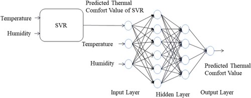ε represents the maximum deviation between $f\left(x_i\right)$ and y. The optimal parameters w and b are obtained by solving the above constrained problems. Then, we train an SVR-DNN model to predict thermal comfort. The structure diagram of SVR-DNN is shown in Figure 2. The inputs of SVR-DNN are predicted value of SVR, indoor temperature and indoor humidity. The output of SVR-DNN is the predicted thermal comfort value. Thus, we predict the occupants' thermal comfort value at time slot t as: (13) $M_{SVR-DN{N}_t}={\mathrm{\Psi }}_{SVR-DNN}(M_{SV{R}_t},T_t,H_t),$(13) where $M_{SVR-DN{N}_t}$ represents the predicted value of thermal comfort at time slot t and ${\mathrm{\Psi }}_{SVR-DNN}$ is the thermal comfort prediction model. The reason why we take the predicted value of SVR model as an input is that we give an approximate label value to the deep neural network in advance, so that the deep neural network can learn more information. The predicted value of SVR has certain guiding significance for the learning of the deep neural network. The single deep neural network has only two feature inputs, while SVR-DNN has three inputs, in which the predicted value of SVR has the feature of the real label. Therefore, SVR-DNN has better performance.

Figure 2. The structure of SVR-DNN for predicting thermal comfort. The inputs of SVR-DNN are predicted value of SVR, indoor temperature and indoor humidity. The output of SVR-DNN is the predicted thermal comfort value.

4.3. Mapping multi-zone residential HVAC control problem into MDP

In this paper, we consider a multi-zone residential apartment in the cooling season. The indoor temperature of the apartment will vary with the setpoint of the HVAC. If the indoor temperature is higher than the set temperature, the HVAC system will work to push the indoor temperature close to the setpoint, on the contrary, HVAC will not operate. The time is denoted as $t=0,1,2\dots$. The duration of each time slot is one hour. We formulate the multi-zone residential HVAC control problem as an MDP, including state, action and reward function.

1. State space

   The state space is shown in Table 2, which includes outdoor temperature, outdoor humidity, thermal comfort and ideal thermal comfort in three zones. Note that state space includes ideal thermal comfort which can change with time. In reality, user's thermal comfort is different in different time periods. In this study, first consider the satisfaction of thermal comfort, and then consider energy saving.

2. Action space

   The action space is shown in Table 3, which includes the temperature setpoints in three zones. HVAC systems will take actions according to different demands. In DQN and Q-learning, the action space is discrete, so we discretise the range of setpoints with a step size of ${0.5}^{\circ }$C. In this study, the set point of relative humidity is fixed and set at 60%.

3. Reward function

   Because it is necessary to consider energy saving under the condition of satisfying thermal comfort requirements, we define the reward function as: (14) $r_t=-(\text{β}\sum _k|M_{Roomk\left(t\right)}-M_{Roomk-ideal\left(t\right)}|+\sum _k{Q}_t^k)/153,k=1,3,5,$(14) where $Q_t^k$ represents the energy consumption of Roomk at time t. Since thermal comfort is the first consideration, multiply the first item by weight β to increase its impact on the reward function.

Table 2. State space.

Parameter	Notation
Outdoor temperature	$T_{out\left(t\right)}$
Outdoor humidity	$H_{out\left(t\right)}$
Thermal comfort of Room1	$M_{Room1\left(t\right)}$
Thermal comfort of Room3	$M_{Room3\left(t\right)}$
Thermal comfort of Room5	$M_{Room5\left(t\right)}$
Ideal thermal comfort for Room1	$M_{Room1-ideal\left(t\right)}$
Ideal thermal comfort for Room3	$M_{Room3-ideal\left(t\right)}$
Ideal thermal comfort for Room5	$M_{Room5-ideal\left(t\right)}$

Table 3. Action space.

Parameter	Notation	range	Unit
Room1 setpoint temperature	$T_{Room1}^{set}$	$[23,27]$	${}^{\circ }$C
Room3 setpoint temperature	$T_{Room3}^{set}$	$[23,27]$	${}^{\circ }$C
Room5 setpoint temperature	$T_{Room5}^{set}$	$[23,27]$	${}^{\circ }$C

4.4. Q-learning, DQN and DDPG algorithms for HVAC thermal comfort control strategies

We implement three algorithms: Q-learning, DQN and DDPG. See Algorithms 1– 3 for the specific algorithm flow.

Algorithm 1 is Q-learning for HVAC control. In Algorithm 1, first initialise the Q value; Q-learning RL agent observes the state $s_t$, selects the action $a_t$ by $ϵ-greedy$ policy, and then updates the Q value by the i.e. “(3(3) $Q(s_t,a_t)=Q(s_t,a_t)+\alpha \left(r_t\right(s_t,a_t)+\gamma \underset{a_{t+1}}{max}Q(s_{t+1},a_{t+1})-Q(s_t,a_t\left)\right)$(3) )”, stores the updated Q value into the Q table, and loops in this way until the state is terminated to jump out of the loop for the next episode update. Algorithms 2 and 3 are DQN and DDPG for HVAC control respectively. In Algorithm 2, the Q-network is initialised and the associated target Q-network is initialised with the same parameters. For each iteration, the state is first initialised and the Q-network selects the action, i.e. the current setpoint, based on the current state by $ϵ-greedy$ policy. Next, the reward and the next state are observed. If Room1 and Room3 are occupied, the transition ($s_t,a_t,r_t,s_{t+1}$) is stored in the replay buffer $D1$; Room5 is occupied, the transition ($s_t,a_t,r_t,s_{t+1}$) is stored in the replay buffer $D2$. When enough samples are collected in the replay buffer, a mini-batch of transitions is randomly selected to update the Q-network parameters. The Q-network parameters are copied to the target Q-network every U time steps of delay. In Algorithm 3, the actor network and critic network are initialised, and the target actor network and target critic network are initialised with the same parameters. Similar to DQN, the state is also initialised; the agent selects $a_t$ through the actor network based on the current state $s_t$, and adds noise to the selected action. The action $a_t$ is executed in the environment, and the reward and next state are observed. The transition ($s_t,a_t,r_t,s_{t+1}$) is stored in the same way as the DQN. Again when enough samples are collected in the replay buffer, a mini-batch of transitions is randomly selected to update the network parameters. The critic network updates the network parameters by the mean square error of the target Q value and the current Q value. The actor network updates the network parameters according to the deterministic policy gradient theorem. To ensure the stability of the algorithm, then the target network parameters are updated softly according to i.e. “(11(11) $\{\begin{array}{ll}{\theta }^{Q^{\mathrm{\prime }}}\leftarrow \tau {\theta }^Q+(1-\tau ){\theta }^{Q^{\mathrm{\prime }}},& \\ {\theta }^{{\mu }^{\mathrm{\prime }}}\leftarrow \tau {\theta }^{\mu }+(1-\tau ){\theta }^{{\mu }^{\mathrm{\prime }}},& 0<\tau \ll 1\end{array}$(11) )”.

5. Simulation environment

The plain layout of a five-zone and three-occupant residential HVAC model (Deng et al., 2019) is shown in Figure 3. There are five rooms in the apartment, of which three are functional rooms, including Room1, Room3 and Room5 which have HVAC systems. The layout of the residential apartment is identified from multi-level residential buildings in Chongqing, China. We use real-world weather data from Bureau (2005). The HVAC model considered in this paper is only utilised for cooling and we consider the cooling time from May to September.

Figure 3. Plain layout of the 3-occupant apartment.

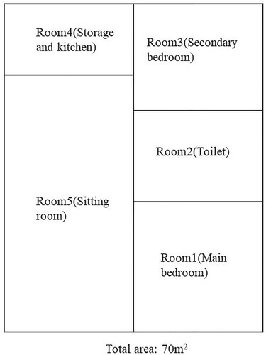
Considering the occupation of personnel, the specific schedule is shown in Table 4. As the toilet and kitchen are occupied only under specific circumstances, these two rooms are not considered for the time being. Both Room1 and Room3 are bedrooms. There are two occupants when Room1 is occupied and one occupant when Room3 is occupied. Room5 is the sitting room, with three occupants when occupied. We assume that the three occupants have the same attributes. It is further assumed that the thermal comfort of occupants changes circularly in a day according to the number of occupants and occupation time. The specific planning is shown in Table 5.

Table 4. Occupation schedule.

Room	Occupation time	Number of occupants
Room1	20:00–24:00, 0:00–7:00	2
Room3	20:00–24:00, 0:00–7:00	1
Room5	7:00–20:00	3

Table 5. Time schedule.

Room	Occupation time	Occupant	Ideal thermal comfort
Room1	0:00–7:00	2	0.15
Room1	7:00–20:00	/	0.35
Room1	20:00–24:00	2	0.1
Room3	0:00–7:00	1	0.2
Room3	7:00–20:00	/	0.35
Room3	20:00–24:00	1	0.15
Room5	0:00–7:00	/	0.35
Room5	7:00–20:00	3	-0.1
Room5	20:00–24:00	/	0.35

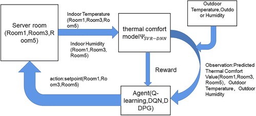
The specific simulation process is shown in Figure 4. Data on the indoor temperature and humidity are collected and fed into a trained SVR-DNN thermal comfort model to predict the current thermal comfort value. The predicted thermal comfort value is used as part of the state and the current reward is obtained through the reward function we designed. Through continuous interaction with the environment and learning, RL agents learn the optimal thermal comfort control strategies for multi-zone HVAC control.

Figure 4. Flowchart of Multi-zone Residential Apartment Simulation.

6. Experiment

In this section, A multi-zone HVAC model is used to demonstrate the effectiveness of RL methods by comparing with the RBC case. And the effectiveness of DDPG for thermal comfort control is demonstrated by comparing with discrete control methods based on DQN and Q-learning. We also compare the performance under different thermal comfort models on the test set to validate the advantages of our method.

6.1. Implementation details

In Q-learning and DQN, the action space is discrete. We discretise the range of setpoints with a step size of 0.5${}^{\circ }$C. As a result, there are 9 actions for each zone and 729 combinations of actions for the 3-zone HVAC. In DDPG and DQN, the specific design of the deep neural network and hyperparameters is respectively shown in Tables 8 and 7. The hyperparameters of Q-learning are shown in Table 6. We design an RBC case which is presented in Table 10 without the RL agent as comparison. When the room is unoccupied, setpoint is set at 27 ${}^{\circ }$C. In other cases, setpoint is set according to Table 10. The implementation details of SVR-DNN are shown in Table 9. We choose Relu as the activation function of hidden layers to prevent the disappearance of the gradient. Since the range of thermal comfort is $[-3,3]$, we choose to use tanh function $y_{tanh}$ as the activation function of the output layer, so that the predicted value is $M=3y_{tanh}$.

Table 6. Q-learning hyperparameters.

Learning rate	${10}^{-3}$
Discount factor (γ)	0.9
Epsilon	0.1

Table 7. DQN hyperparameters.

Size of input	8
No. of hidden layers	2
Size of each hidden layer	[8,128], [128,64]
Size of output	1
Activation function	Relu
Optimiser	Adam
Learning rate	${10}^{-3}$
Batch size	64
Discount factor (γ)	0.9
Buffer size	20000
Delayed policy update U	2

Table 8. DDPG hyperparameters.

Critic networks	$11\to 128\to 64\to 1$
Actor networks	$8\to 128\to 64\to 3$
Activation function	Actor (Tanh) critic (Relu)
Optimiser	Adam
Learning rate	${10}^{-3}$
Batch size	64
TAU τ	0.005
Discount factor (γ)	0.9
Buffer size	20000
Exploration noise	$\mathcal{N}$(0,0.5)

Table 9. The implementation details of SVR-DNN.

Networks	$3\to 128\to 64\to 1$
Activation function of hidden layers	Relu
Optimiser	Adam
Learning rate	${10}^{-3}$
Batch size	64
Activation function of output layer	$3\ast Tanh$

Table 10. RBC.

Room	Occupation time	Occupant	Setpoint value
Room1	0:00–7:00	2	25${}^{\circ }$C
Room1	7:00–20:00	/	27${}^{\circ }$C
Room1	20:00–24:00	2	24${}^{\circ }$C
Room3	0:00–7:00	1	25${}^{\circ }$C
Room3	7:00–20:00	/	27${}^{\circ }$C
Room3	20:00–24:00	1	24${}^{\circ }$C
Room5	0:00–7:00	/	27${}^{\circ }$C
Room5	7:00–20:00	3	24${}^{\circ }$C
Room5	20:00–24:00	/	27${}^{\circ }$C

6.2. Performance of SVR-DNN

We select 899 samples under the same conditions in the ASHRAE (Fldvry Liina et al., 2018), 80% for training and 20% for testing. These samples are selected in summer and under the condition of indoor air conditioning. We first train an SVR model. Then we take the predicted value of SVR, indoor temperature and indoor humidity as the input of the deep neural network. The occupants' thermal comfort value at time slot t as (15) $M_t={\mathrm{\Psi }}_{SVR-DNN}(M_{SV{R}_t},T_t,H_t).$(15)

The prediction error is shown in Table 11 below. These datasets are labelled by the target subjects in different thermal states to evaluate their thermal comfort values. Because of individual physiological differences, regional differences and other factors, the labelled data may be subjective and noisy. In order to solve the above problems, we add L2 regularisation to SVR-DNN to solve the overfitting problem, so that SVR-DNN has better generalisation ability. The cost function of SVR-DNN with L2 regularisation is as follows: (16) $L_{{\mathrm{\Psi }}_{SVR-DNN}}=\frac{1}{n}\sum _{i=1}^n(M_i-M_i^{\mathrm{\prime }}{)}^2+\frac{\lambda }{2n}\sum _{j=1}^m\Vert {\omega }_j{\Vert }_2^2,$(16) where n is the number of training samples, $M_i$ is the ith label value, and $M_i^{\mathrm{\prime }}$ is the predicted value of SVR-DNN. In i.e. “(16(16) $L_{{\mathrm{\Psi }}_{SVR-DNN}}=\frac{1}{n}\sum _{i=1}^n(M_i-M_i^{\mathrm{\prime }}{)}^2+\frac{\lambda }{2n}\sum _{j=1}^m\Vert {\omega }_j{\Vert }_2^2,$(16) )”, The second term is the regular term. λ is the weight of the regular term. The greater λ is, the greater the role of the regular term, that is, the greater the punishment. m is the number of weights in the neural network, and ${\omega }_j$ is the jth weight. We set $\lambda =0.01$. The prediction errors of DNN and SVR-DNN are shown in Figure 5. The prediction performance improvement of SVR-DNN compared with other methods is shown in Table 12. SVR-DNN shows the best performance.

Figure 5. The convergence and comparison of DNN and SVR-DNN for thermal comfort prediction. The horizontal axis represents the number of epochs / 5, and the loss of the vertical axis represents the prediction error(MSE).

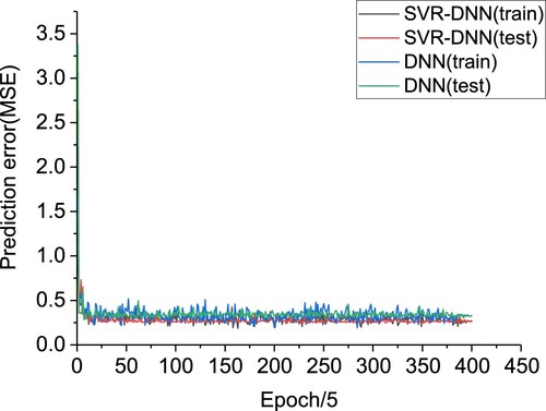
Table 11. Prediction error.

Model	DNN	SVR	XGBoost	Linear Regression	SVR-DNN
Prediction error (MSE)	0.329204	0.306900	0.336993	0.342541	0.261614

Table 12. The prediction performance improvement of SVR-DNN.

	DNN	SVR	XGBoost	Linear Regression
SVR-DNN	20.5%	14.6%	22.4%	23.6%

6.3. Performance of DDPG based on SVR-DNN

1. Convergence

   In Figure 6, the reward of Q-learning, DQN and DDPG is presented during training. In this paper, we take May to September as an episode, a total of 50 training episodes. We set the weight β in the reward function to 10. From Figure 6, we note that the rewards of DQN and DDPG are lower than those of Q-learning in the first few episodes. This is because both DQN and DDPG need to store transitions in the early stage, and they have not learned yet. On the contrary, Q-learning has begun to learn. After about 15 episodes, Q-learning tends to converge, which is due to the discretization of state space and action space, which greatly reduces the scope of exploration and converges quickly. However, the reduction of exploration space will lead to insufficient exploration, resulting in low reward. The reward of Q-learning is the lowest of the three methods. The reward of DQN tends to converge after about 24 episodes. Due to the discretization of action space and the incomplete exploration of action space combination, the reward of DQN is lower than that of DDPG. Because DDPG can deal with continuous control problems, it can explore enough space so that it can find the optimal action to get a higher reward. The reward of DDPG is the highest of the three methods.

   The violation of thermal comfort in each episode is presented in Figure 7. The thermal comfort violation and reward have the opposite trend. The lower the thermal comfort violation, the higher the reward, which also indicates the better the thermal comfort control strategy learned by the RL agent. The violation of thermal comfort has the same convergence trend as the reward. The Q-learning method had the highest thermal comfort violation, followed by DQN and the least by DDPG. It can be seen from Figures 6 and 7 that the DDPG method has greater advantages in dealing with HVAC control problems. Both Q learning and DQN do not perform as well as the DDPG method, which is better able to meet the thermal comfort needs of occupants.

2. Computational efficiency

   The code of thermal comfort model training and RL algorithms is written in Python 3.7 with the deep learning open-source platform pytorch. The hardware environment we use is a laptop with Intel CoreTM i5-9300H 2.40 GHz CPU and an NVIDIA GTX 1650Ti.

3. Analysis and comparison with different control methods

   The indoor temperature based on Q-learning, DQN and DDPG methods is presented in Figures 8(a), 9(a) and 10(a) respectively in Changsha. Notice that there is a period of relatively low temperature between 0 to 1000 hours and 3000 to 4000 hours. This is because HVAC is not on, the indoor temperature is relatively low and does not reach the setpoint temperature. The indoor temperature controlled by DDPG is mostly between ${25}^{\circ }$C and ${26.5}^{\circ }$C from Figure 8(a). In Figures 9(a) and 10(a), part of the indoor temperature controlled by DQN is biased to ${24.5}^{\circ }$C and ${27}^{\circ }$C and the part of that controlled by Q-learning is biased to ${24}^{\circ }$C. We take out the indoor temperature and thermal comfort on August 1 for detailed description and analysis. From Figures 11(a) and 12, the indoor temperature and thermal comfort controlled by the DDPG method are more regular, and the thermal comfort deviates little from the ideal thermal comfort we set. In Figure 11(b), the temperature controlled by DQN is lower than that controlled by DDPG most of the day, which increases energy consumption. The performance of indoor temperature controlled by Q-learning is worse than that of DQN and DDPG from Figure 11(c). In Figure 12, the comparison of thermal comfort of three rooms is presented on August 1. DDPG method maintained thermal comfort best in three rooms. DQN can learn a certain amount of laws, but it can't learn more complete knowledge. Only partial thermal comfort can be maintained on this day by DQN. Q-learning can only maintain a small part of thermal comfort in a day because it can only explore a limited space. The maintenance of thermal comfort from May to September is presented based on DDPG, DQN and Q-learning in Figures 8(b), 9(b) and 10(b).

   The well-trained RL agents are applied to generate the HVAC control strategies for the test 21 days from July 20 to August 9 in Chongqing. The RL control strategy, the associated indoor temperature and thermal comfort are further shown in Figures 13– 15. In Figure 13, the control strategy of the DDPG RL agent is well able to learn the key knowledge of the environment. The indoor temperature and the thermal comfort level show regularity, and the DDPG agent is able to control the thermal comfort to fluctuate around the ideal comfort level we set and to achieve energy savings. As shown in Figures 14 and 15, DQN can learn certain laws, and since they both can only handle discrete action spaces, especially Q-learning can only handle discrete problems. They all end up learning worse strategies than DDPG. We take out the indoor temperature and thermal comfort based on four methods on August 1 in Chongqing. In Figures 16 and 17, the DDPG method continues to show the best performance and is able to learn and make optimal actions in complex environments. DQN and Q-learning are also unable to handle the continuous action space and explore all actions, so their performance is worse than DDPG. Especially the strategy learned by Q-learning has poor regularity. RBC is usually set based on experience and can not learn from historical data to self-regulate, so it has a high degree of violation. In particular, Q- learning, when the environment is too complex to handle, is not necessarily better than RBC in terms of the strategies it eventually learns.

   The thermal comfort violation and energy consumption test results of the four methods are shown in Table 13. In Table 13, The DDPG control method has the lowest energy consumption and the least thermal comfort violation. Although the energy consumption of DQN and Q-learning is slightly higher than that of RBC, the thermal comfort violation is smaller than that of RBC. Compared with Q-learning and DQN, DDPG can reduce the energy consumption cost by 4.69%, 3.52% and reduce the comfort violation by 68.11%, 64.37%; compared with RBC, DDPG, DQN and Q-learning based on SVR-DNN reduce thermal comfort violation by 69.27%, 13.76%, 3.63%. DDPG can better find the balance between thermal comfort and energy consumption. The thermal comfort violation for each room during each time period is shown in Table 14. The thermal comfort violation between 7:00 and 20:00 in Room5 is larger in all four methods, which may be due to the large time span. Except for DDPG, DQN outperforms Q-learning and RBC in all time periods. Table 15 shows the average values of thermal comfort in each room for each time period. The average thermal comfort of DDPG deviates the least from the ideal thermal comfort, while all other methods deviate in all degrees.

4. Performance comparison under different thermal comfort models

   We use different thermal comfort models to compare their effects on energy consumption as well as thermal comfort. The test results are shown in the Table 16. A comparison of Tables 13 and 16 shows that both the DNN and SVR based models have higher thermal comfort violation and energy consumption than the SVR-DNN based model. Also under the DDPG method, the SVR-DNN model can reduce energy consumption by 6% and 4.7% compared with DNN and SVR. The associated indoor temperature and thermal comfort based on DNN and SVR are shown in Figures 18– 23. We can see from these figures that the control strategy based on the DNN as well as the SVR model, i.e. the temperature set point, is significantly lower which leads to increased energy consumption. The thermal comfort predicted by the SVR and DNN models is higher than that predicted by the SVR-DNN, which results in a lower temperature setpoint learned by RL agents. The more accurately the thermal comfort is predicted, the better the optimal control strategy for RL will also be. Table 17 shows the thermal comfort violation in the room for each time period based on the DNN and SVR models respectively. Table 18 shows the average values of thermal comfort in each room for each time period. The DDPG method also demonstrates the best control performance as seen in Tables 17 and 18. The comparison between Tables 14 and 17 shows that RL-based thermal comfort control strategies are able to reduce thermal comfort violation regardless of the thermal comfort model. The DDPG method performs better than the discrete methods DQN and Q-learning regardless of the thermal comfort model. Our method can better meet the thermal comfort requirements of occupants and also achieve energy savings with less thermal comfort violation.

Figure 6. Convergence of different RL methods.

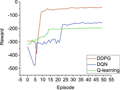
Figure 7. Convergence of violation of thermal comfort via different RL methods.

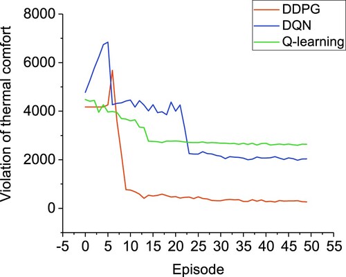
Figure 8. Indoor temperature and thermal comfort by DDPG from May to September in Changsha. (a) Indoor temperature. (b) Thermal comfort.

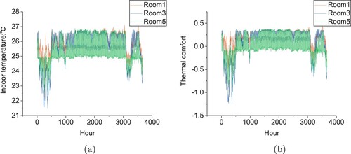
Figure 9. Indoor temperature and thermal comfort by DQN from May to September in Changsha. (a) Indoor temperature. (b) Thermal comfort.

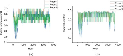
Figure 10. Indoor temperature and thermal comfort by Q-learning from May to September in Changsha. (a) Indoor temperature. (b) Thermal comfort.

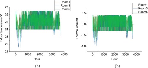
Figure 11. Indoor temperature on August 1 in Changsha. (a) DDPG. (b) DQN. (c) Q-learning.

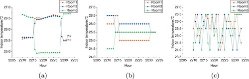
Figure 12. Thermal comfort on August 1 in Changsha. (a) Room1. (b) Room3. (c) Room5.

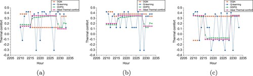
Figure 13. Room1 for 21 test days based on SVR-DNN.

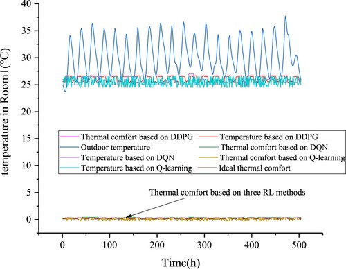
Figure 14. Room3 for 21 test days based on SVR-DNN.

Figure 15. Room5 for 21 test days based on SVR-DNN.

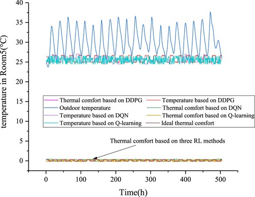
Figure 16. Indoor temperature on August 1 in Chongqing based on SVR-DNN. (a) Room1. (b) Room3. (c) Room5.

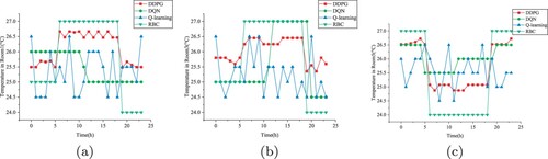
Figure 17. Thermal comfort on August 1 in Chongqing based on SVR-DNN. (a) Room1. (b) Room3. (c) Room5.

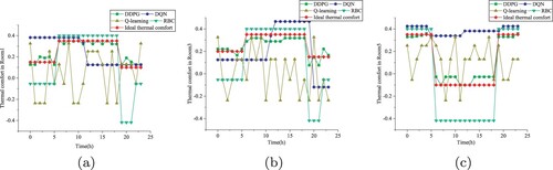
Figure 18. Room1, Room2 and Room3 for 21 test days based on DNN. (a) Room1. (b) Room3. (c) Room5.

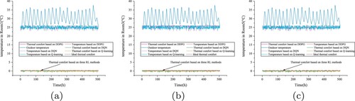
Figure 19. Indoor temperature on August 1 in Chongqing based on DNN. (a) Room1. (b) Room3. (c) Room5.

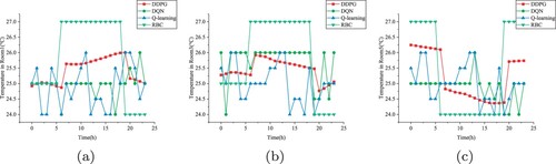
Figure 20. Thermal comfort on August 1 in Chongqing based on DNN. (a) Room1. (b) Room3. (c) Room5.

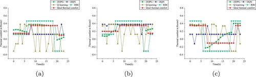
Figure 21. Room1, Room2 and Room3 for 21 test days based on SVR. (a) Room1. (b) Room3. (c) Room5.

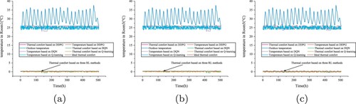
Figure 22. Indoor temperature on August 1 in Chongqing based on SVR. (a) Room1. (b) Room3. (c) Room5.

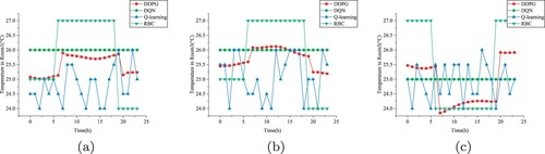
Figure 23. Thermal comfort on August 1 in Chongqing based on SVR. (a) Room1. (b) Room3. (c) Room5.

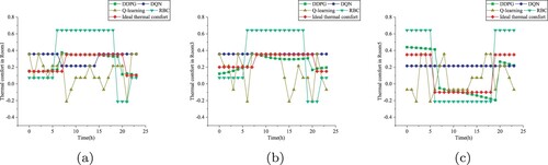
Table 13. Test results different HVAC control methods based on SVR-DNN.

Control method	DDPG	DQN	Q-learning	RBC
Energy consumption (kWh/m${}^2$)	13.78	14.28	14.45	14.03
Thermal comfort violation	105.03	294.75	329.34	341.76

Table 14. Thermal comfort violation for each room time period in test days based on SVR-DNN.

Room	Time	DDPG	DQN	Q-learning	RBC
Room1	0:00–7:00	12.01	24.95	28.75	35.55
	7:00–20:00	11.7	31.24	63.52	44.86
	20:00–24:00	3.72	11.57	11.15	17.33
Room3	0:00–7:00	7.42	27.48	32.29	40.15
	7:00–20:00	20.97	38.92	60.83	44.02
	20:00–24:00	2.06	10.96	10.53	20.48
Room5	0:00–7:00	19.11	23.68	44.36	42.04
	7:00–20:00	27.14	109.49	62.55	94.3
	20:00–24:00	0.87	16.46	15.36	3.03

Table 15. The average value of thermal comfort for each room time period in test days based on SVR-DNN.

Room	Time	Metric	DDPG	DQN	Q-learning	RBC
Room1	0:00–7:00	Mean	0.206296925	0.279399627	0.083509644	0.049563237
	7:00–20:00	Mean	0.307454857	0.268232478	0.119496962	0.2672754
	20:00–24:00	Mean	0.159069733	0.283710488	0.090178026	−0.175217673
Room3	0:00–7:00	Mean	0.22098829	0.215197303	0.073447687	0.057577235
	7:00–20:00	Mean	0.273166488	0.255532399	0.135571265	0.274897414
	20:00–24:00	Mean	0.166890588	0.20246808	0.108376095	−0.175217673
Room5	0:00–7:00	Mean	0.241993896	0.227699292	0.090051476	0.16688822
	7:00–20:00	Mean	-0.001009323	0.297996822	0.066989154	−0.292768931
	20:00–24:00	Mean	0.344233155	0.10578414	0.109335237	0.397936726

Table 16. Test results under different thermal comfort models.

Control method	DDPG-SVR-DNN	DDPG-DNN	DDPG-SVR	DQN-DNN	DQN-SVR	Q-learning-DNN	Q-learning-SVR
Energy consumption (kWh/m${}^2$)	13.78	14.66	14.47	14.45	14.7	15.42	15.32
Thermal comfort violation	105.03	106.53	106.08	320.86	296.95	338.95	337.74

Table 17. Thermal comfort violation for each room time period in test days based on DNN and SVR.

Room	Time	DDPG-DNN	DDPG-SVR	DQN-DNN	DQN-SVR	Q-learning-DNN	Q-learning- SVR
Room1	0:00–7:00	16.02	7.89	17.69	33.81	36.43	27.56
	7:00–20:00	9.02	11.76	73.46	45.09	62.96	68.79
	20:00–24:00	4.69	3.73	5.37	13.62	13.74	11.55
Room3	0:00–7:00	19.27	10.8	37.3	24.14	34.83	28.49
	7:00–20:00	10.32	14.51	36.01	30.67	58.85	72.6
	20:00–24:00	8.04	3.88	16.12	13.43	14.8	10.81
Room5	0:00–7:00	12.08	20.71	50.02	37.55	38.09	42.5
	7:00–20:00	24.84	27.94	68.88	80.27	64.4	57.43
	20:00–24:00	2.25	4.86	16.01	18.37	14.75	18.01

Table 18. The average value of thermal comfort for each room time period in test days based on DNN and SVR.

Room	Time	Metric	DDPG-DNN	DDPG-SVR	DQN-DNN	DQN-SVR	Q-learning-DNN	Q-learning-SVR
Room1	0:00–7:00	Mean	0.176121071	0.163330232	0.070939637	0.176376879	0.099500439	0.104587748
	7:00–20:00	Mean	0.342919457	0.317404587	0.082962213	0.191363214	0.134131976	0.101705839
	20:00–24:00	Mean	0.107864567	0.151180513	0.08415923	0.195012061	0.071357839	0.05948347
Room3	0:00–7:00	Mean	0.268783972	0.220472037	0.285020506	0.236517691	0.146592257	0.118777229
	7:00–20:00	Mean	0.350937599	0.333535993	0.267414959	0.246095914	0.151241922	0.087110452
	20:00–24:00	Mean	0.226245187	0.198865825	0.280859174	0.267293975	0.099217035	0.093365618
Room5	0:00–7:00	Mean	0.298273336	0.299004445	0.053426388	0.129701557	0.137928131	0.100743801
	7:00–20:00	Mean	−0.029416712	−0.041625831	0.063154792	0.151225901	0.041768979	0.060525998
	20:00–24:00	Mean	0.368325034	0.37592818	0.095797246	0.05948347	0.133740349	0.0662599

7. Conclusion

In this paper, we proposed a method combining a thermal comfort prediction model and deep reinforcement learning to optimise the residential multi-zone HVAC control. We first trained an SVR-DNN model to predict thermal comfort; then used DDPG based on SVR-DNN to optimise indoor thermal comfort to meet occupants' conditions and achieve energy savings. A multi-zone residential HVAC model was used to evaluate the performance of the method we proposed. The results show that SVR-DNN can improve thermal comfort prediction performance by 20.5% compared with the deep neural network(DNN); compared with Q-learning and DQN, DDPG can reduce the energy consumption cost by 4.69%, 3.52% and reduce the comfort violation by 68.11%, 64.37%; based on SVR-DNN, DDPG, DQN and Q-learning compared with a rule-based control strategy can respectively reduce thermal comfort violation by 69.27%, 13.76%, 3.63%. The optimal control based on SVR-DNN thermal comfort model shows the best performance. Through comparative experiments, Q-learning shows great limitations for handling complex HVAC environment problems;compared with Q-learning, DQN shows better performance; DDPG shows the best performance.

In future work, we consider multi-agent RL algorithms to solve the multi-zone HVAC control problem. Instead of limiting the consideration of energy saving comfort optimisation to the cooling season, we are able to carry out energy saving optimisation control of thermal comfort on a year-round basis.

Disclosure statement

The authors declare that the research was conducted in the absence of any commercial or financial relationships that could be construed as a potential conflict of interest.

Additional information

Funding

This work was financially supported by Primary Research and Development Plan of China [grant number 2020YFC2006602], National Natural Science Foundation of China [grant numbers 62072324, 61876217, 61876121, 61772357], University Natural Science Foundation of Jiangsu Province [grant number 21KJA520005], Primary Research and Development Plan of Jiangsu Province [grant number BE2020026], Natural Science Foundation of Jiangsu Province [grant number BK20190942].

References

- Ahn, K. U., & Park, C. S. (2019). Application of deep Q-networks for model-free optimal control balancing between different HVAC systems. Science and Technology for the Built Environment, 26(1), 1–16. https://doi.org/10.1080/23744731.2019.1680234
- Baldi, S., Korkas, C. D., Lv, M., & Kosmatopoulos, E. B. (2018). Automating occupant-building interaction via smart zoning of thermostatic loads: A switched self-tuning approach. Applied Energy, 231, 1246–1258. https://doi.org/10.1016/j.apenergy.2018.09.188
- Brandi, S., Piscitelli, M. S., Martellacci, M., & Capozzoli, A. (2020). Deep reinforcement learning to optimise indoor temperature control and heating energy consumption in buildings. Energy and Buildings, 224, Article ID 110225. https://doi.org/10.1016/j.enbuild.2020.110225
- Bureau, C. M. (2005). China standard weather data for analyzing building thermal conditions (pp. 90–105). China Building Industry Publishing House.
- Chen, Z., Wang, C., Jin, H., Li, J., Zhang, S., & Ouyang, Q. (2022). Hierarchical-fuzzy allocation and multi-parameter adjustment prediction for industrial loading optimisation. Connection Science, 34(1), 687–708. https://doi.org/10.1080/09540091.2022.2031887
- Cicirelli, F., Guerrieri, A., Mastroianni, C., Scarcello, L., Spezzano, G., & Vinci, A. (2021). Balancing energy consumption and thermal comfort with deep reinforcement learning. In 2021 IEEE 2nd international conference on human-machine systems (ICHMS) (pp. 1–6). IEEE.
- Costa, A., Keane, M. M., Torrens, J. I., & Corry, E. (2013). Building operation and energy performance: Monitoring, analysis and optimisation toolkit. Applied Energy, 101(JAN), 310–316. https://doi.org/10.1016/j.apenergy.2011.10.037
- Deng, J., Yao, R., Yu, W., Zhang, Q., & Li, B. (2019). Effectiveness of the thermal mass of external walls on residential buildings for part-time part-space heating and cooling using the state-space method. Energy and Buildings, 190, 155–171. https://doi.org/10.1016/j.enbuild.2019.02.029
- Du, Y., Zandi, H., Kotevska, O., Kurte, K., Munk, J., Amasyali, K., Mckee, E., & Li, F. (2021). Intelligent multi-zone residential HVAC control strategy based on deep reinforcement learning. Applied Energy, 281, Article ID 116117. https://doi.org/10.1016/j.apenergy.2020.116117
- Fatema, I., Kong, X., & Fang, G. (2021). Electricity demand and price forecasting model for sustainable smart grid using comprehensive long short term memory. International Journal of Sustainable Engineering, 14(6), 1714–1732. https://doi.org/10.1080/19397038.2021.1951882
- Fu, Q., Chen, X., Ma, S., Fang, N., Xing, B., & Chen, J. (2022). Optimal control method of HVAC based on multi-agent deep reinforcement learning. Energy and Buildings, 270, Article ID 112284. https://doi.org/10.1016/j.enbuild.2022.112284
- Fldvry Liina, V., Cheung, T., Zhang, H., de Dear, R., Parkinson, T., Arens, E., Chun, C., Schiavon, S., Luo, M., Brager, G., & Li, P. (2018). Development of the ASHRAE global thermal comfort database II. Building and Environment, 142, 502–512. https://doi.org/10.1016/j.buildenv.2018.06.022
- Han, X., He, H., Wu, J., Peng, J., & Li, Y. (2019). Energy management based on reinforcement learning with double deep Q-learning for a hybrid electric tracked vehicle. Applied Energy, 254, Article ID 113708. https://doi.org/10.1016/j.apenergy.2019.113708
- Jiang, Z., Risbeck, M. J., Ramamurti, V., Murugesan, S., Amores, J., Zhang, C., Lee, Y. M., & Drees, K. H. (2021). Building HVAC control with reinforcement learning for reduction of energy cost and demand charge. Energy and Buildings, 239, Article ID 110833. https://doi.org/10.1016/j.enbuild.2021.110833
- Kheyrinataj, F., & Nazemi, A. (2020). Fractional power series neural network for solving delay fractional optimal control problems. Connection Science, 32(1), 53–80. https://doi.org/10.1080/09540091.2019.1605498
- Korkas, C. D., Baldi, S., & Kosmatopoulos, E. B. (2018). 9-grid-connected microgrids: Demand management via distributed control and human-in-the-loop optimization. In I. Yahyaoui (Ed.), Advances in renewable energies and power technologies (pp. 315–344). Elsevier. https://doi.org/10.1016/B978-0-12-813185-5.00025-5
- Korkas, C. D., Baldi, S., Michailidis, I., & Kosmatopoulos, E. B. (2015). Intelligent energy and thermal comfort management in grid-connected microgrids with heterogeneous occupancy schedule. Applied Energy, 149(C), 194–203. https://doi.org/10.1016/j.apenergy.2015.01.145
- Kurte, K., Munk, J., Amasyali, K., Kotevska, O., Cui, B., Kuruganti, T., & Zandi, H. (2020). Electricity pricing aware deep reinforcement learning based intelligent HVAC control. In Proceedings of the 1st international workshop on reinforcement learning for energy management in buildings & cities (pp. 6–10). Association for Computing Machinery. https://doi.org/10.1145/3427773.3427866.
- Kurte, K., Munk, J., Kotevska, O., Amasyali, K., Smith, R., McKee, E., Du, Y., Cui, B., Kuruganti, T., & Zandi, H. (2020). Evaluating the adaptability of reinforcement learning based HVAC control for residential houses. Sustainability, 12(18), Article ID 7727. https://doi.org/10.3390/su12187727
- Kurte, K. R., Amasyali, K., Munk, J. D., & Zandi, H. (2021). Comparative analysis of model-free and model-based HVAC control for residential demand response. In Proceedings of the 8th ACM international conference on systems for energy-efficient buildings, cities, and transportation.
- Lillicrap, T. P., Hunt, J. J., Pritzel, A., Heess, N., Erez, T., Tassa, Y., Silver, D., & Wierstra, D. (2015). Continuous control with deep reinforcement learning. Computer Science. arXiv preprint arXiv:1509.02971
- Liu, W., Lian, Z., & Zhao, B. (2007). A neural network evaluation model for individual thermal comfort. Energy and Buildings, 39(10), 1115–1122. https://doi.org/10.1016/j.enbuild.2006.12.005
- McKee, E., Du, Y., Li, F., Munk, J., Johnston, T., Kurte, K., Kotevska, O., Amasyali, K., & Zandi, H. (2020). Deep reinforcement learning for residential HVAC control with consideration of human occupancy. In 2020 IEEE power & energy society general meeting (PESGM) (pp. 1–5).
- Montague, P. (1999). Reinforcement learning: An introduction, by Sutton, R.S. and Barto, A.G.. Trends in Cognitive Sciences, 3(9), 360. https://doi.org/10.1016/S1364-6613(99)01331-5
- Moreno, B., Gonzalo, F., & Hernandez, J. A. (2017). Designing a wireless sensor with ultra-capacitor and PV microcell for smart building energy management. International Journal of Embedded Systems, 11(1), 1. https://doi.org/10.1504/IJES.2019.097565
- Nazemi, A., Fayyazi, E., & Mortezaee, M. (2019). Solving optimal control problems of the time-delayed systems by a neural network framework. Connection Science, 31(4), 342–372. https://doi.org/10.1080/09540091.2019.1604627
- Prez-Lombard, L., Ortiz, J., & Pout, C. (2008). A review on buildings energy consumption information. Energy and Buildings, 40(3), 394–398. https://doi.org/10.1016/j.enbuild.2007.03.007
- Qiu, S., Li, Z., Li, Z., Li, J., Long, S., & Li, X. (2020). Model-free control method based on reinforcement learning for building cooling water systems: Validation by measured data-based simulation. Energy and Buildings, 218, Article ID 110055. https://doi.org/10.1016/j.enbuild.2020.110055
- Qiu, S., Li, Z., Li, Z., & Zhang, X. (2020). Model-free optimal chiller loading method based on Q-learning. Science and Technology for the Built Environment, 26(8), 1100–1116. https://doi.org/10.1080/23744731.2020.1757328
- Rocchetta, R., Bellani, L., Compare, M., Zio, E., & Patelli, E. (2019). A reinforcement learning framework for optimal operation and maintenance of power grids. Applied Energy, 241, 291–301. https://doi.org/10.1016/j.apenergy.2019.03.027
- Sang, J., & Sun, H. (2021). HVAC cooling–heating-power demand strategy optimization based on DDPG control. In 2021 IEEE international conference on advances in electrical engineering and computer applications (AEECA) (pp. 266–270).
- Shaw, E. W. (1972). Thermal comfort: Analysis and applications in environmental engineering, by P. O. Fanger. 244 pp. Danish Technical Press. Copenhagen, Denmark, 1970. Danish Kr. 76, 50. The Journal of the Royal Society for the Promotion of Health.
- Silver, D., Lever, G., Heess, N., Degris, T., & Riedmiller, M. (2014). Deterministic policy gradient algorithms. JMLR.org.
- Sutton, R. S., Mcallester, D., Singh, S., & Mansour, Y. (1999). Policy gradient methods for reinforcement learning with function approximation. Submitted to Advances in Neural Information Processing Systems, 12, 1057–1063. https://doi.org/10.5555/3009657.3009806.
- Volodymyr, M., Koray, K., David, S., Rusu, A. A., Joel, V., Bellemare, M. G., Graves, A., Riedmiller, M., Fidjeland, A. K., Ostrovski, G., & Petersen, S. (2019). Human-level control through deep reinforcement learning. Nature, 518(7540), 529–33. https://doi.org/10.1038/nature14236
- Watari, D., Taniguchi, I., Catthoor, F., Marantos, C., Siozios, K., Shirazi, E., Soudris, D., & Onoye, T. (2021). Thermal comfort aware online energy management framework for a smart residential building. In 2021 design, automation & test in Europe conference & exhibition (date) (pp. 535–538).
- Wei, T., Ren, S., & Zhu, Q. (2021). Deep reinforcement learning for joint datacenter and HVAC load control in distributed mixed-use buildings. IEEE Transactions on Sustainable Computing, 6(3), 370–384. https://doi.org/10.1109/TSUSC.2019.2910533
- Wu, X., He, J., Xu, Y., Lu, J., Lu, N., & Wang, X. (2018). Hierarchical control of residential HVAC units for primary frequency regulation. IEEE Transactions on Smart Grid, 9(4), 3844–3856. https://doi.org/10.1109/TSG.2017.2766880
- Yu, L., Sun, Y., Xu, Z., Shen, C., Yue, D., Jiang, T., & Guan, X. (2021). Multi-agent deep reinforcement learning for HVAC control in commercial buildings. IEEE Transactions on Smart Grid, 12(1), 407–419. https://doi.org/10.1109/TSG.5165411
- Yu, L., Xie, W., Xie, D., Zou, Y., & Jiang, T. (2019). Deep reinforcement learning for smart home energy management. IEEE Internet of Things Journal, PP(99), 1–1. https://doi.org/10.1109/JIOT.2019.2957289
- Zeng, T., & Barooah, P. (2020). An autonomous MPC scheme for energy-efficient control of building HVAC systems. In 2020 American control conference (ACC) (pp. 4213–4218).
- Zeng, T., & Barooah, P. (2021). An adaptive MPC scheme for energy-efficient control of building HVAC systems, arXiv abs/2102.03856.
- Zenger, A., Schmidt, J., & Krdel, M. (2013). Towards the intelligent home: Using reinforcement-learning for optimal heating control. Springer.
- Zhou, X., Xu, L., Zhang, J., Niu, B., Luo, M., Zhou, G., & Zhang, X. (2020). Data-driven thermal comfort model via support vector machine algorithms: Insights from ASHRAE RP-884 database. Energy and Buildings, 211, Article ID 109795. https://doi.org/10.1016/j.enbuild.2020.109795
- Zhou, X., Zhu, F., & Zhao, P. (2022). Predicting before acting: Improving policy quality by taking a vision of consequence. Connection Science, 34(1), 608–629. https://doi.org/10.1080/09540091.2022.2025765