Deep and hybrid learning of MRI diagnosis for early detection of the progression stages in Alzheimer’s disease

Abstract

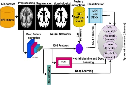
Alzheimer’s, or so-called dementia, is one of the types of diseases that affects brain cells and causes memory loss, difficulty in thinking, and forgetfulness. Thus far, there is no effective treatment for AD, but treatment could be helpful in impeding the progression of the disease. Therefore, early AD diagnosis is effective in limiting the disease from progressing to advanced and dangerous stages. Physicians and radiologists face difficulties in diagnosing healthy nerve cells from soft tissue, and it requires substantial expertise and a long time to decipher the MRI images. Thus, artificial intelligence techniques can play a key role in diagnosing MRI images for early detection of AD. In this study, four proposed systems with different methodologies and materials for tracking the stages of AD development are presented. The first proposed system is to classify a data set using artificial neural networks (ANNs) and feed-forward neural networks (FFNN) based on the features extracted in a hybrid manner by using a combination of Local Binary Pattern (LBP), Discrete Wavelet Transform (DWT), and Gray Level Co-occurrence Matrix (GLCM) algorithms. The second proposed system is to classify the data set using two deep learning models – ResNet-18 and AlexNet – that are pre-trained based on deep feature map extraction. The third proposed system is to diagnose the data set using a hybrid technology between ResNet-18 and AlexNet models to extract feature maps and machine learning (SVM) to classify feature maps. The fourth proposed system diagnoses the data set using ANN and FFNN algorithms based on the hybrid features of ResNet-18 and AlexNet deep learning models and traditional algorithms (LBP, DWT, and GLCM). All the proposed techniques achieved superior results in the diagnosis of MRI images for early detection of AD. The FFNN algorithms based on the hybrid features extracted by ResNet-18 with features extracted using traditional algorithms achieved an accuracy of 99.8%, precision of 99.9%, sensitivity of 99.75%, specificity of 100%, and AUC of 99.94%.

KEYWORDS:

• Deep learning
• neural networks
• machine learning
• hybrid technique
• Alzheimer’s disease
• LBP

1. Introduction

Alzheimer’s disease is a progressive degenerative disease that affects the nervous system through a loss of neurons in the brain (Ulep et al., 2018). Due to the loss of neurons in the brain, higher brain functions gradually deteriorate and, therefore, this affects memory and knowledge with a decrease in motor functions. AD is one of the common kinds of dementia, accounting for approximately 70% of dementia types. Age plays a key role in AD, as most incidences are observed in people over 65 years of age, with a higher infection rate among women than among men (Viña & Lloret, 2010). The etiology remains obscure; however, the major theories are based on the assembly of Aβ peptides outside cells and hyperphosphorylated tau protein inside cells (Zaretsky & Zaretskaia, 2021). These two forms are named amyloid plaques (a protein deposit called beta-amyloid that accumulates in the spaces of neurons) and tangles (twisted protein fibres called “tau” that accumulate inside nerve cells). Biological signs are indicators of the state of the emergence of a few early symptoms of AD before it develops into clinical symptoms (Porsteinsson et al., 2021). Therefore, it is suspected that amyloid plaques and synapses are responsible for the damage to neurons and lead to a gradual loss of memory, with changes in behaviour and thought (Soldan et al., 2017). Despite the development and advanced renaissance in the medical field, effective treatments for AD remain far from being achieved. Nevertheless, certain medicines delay the progression of the disease to advanced stages. AD is also multifactorial, and is not merely related to ageing; it may result from sleep disorders, diet, human lifestyle, genetics, and environmental factors (X. X. Zhang et al., 2021). Preclinical, mild cognitive, and dementia are the three phases of AD. While Alzheimer’s begins for a long period without symptoms, which is called the clinical stage, the clinical stage develops (the progression of the physiological process) with the emergence of vital signs and is more susceptible to infection with MCI; finally, the MCI stage develops until AD appears with all its vital signs (Venugopalan et al., 2021). Biomarkers in the MCI stage are not sufficient to accurately predict stability versus those who will likely develop dementia or AD (Meghdadi et al., 2021). In other words, MCI is the early indication for early diagnosis of cases before progression to AD (Tabatabaei-Jafari et al., 2015). The widespread use of MRI to diagnose the structure of the brain can be of assistance in the early diagnosis of the disease (Nadel et al., 2021). Therefore, doctors and specialists recommend that patients with cognitive impairment undergo imaging of the brain’s internal structure by MRI, which has a vital role in diagnosing AD and dementia (Johnson et al., 2012). The MRI technique offers a scope of various sequences that can identify the inner tissues of the brain. MRI images show measures of brain atrophy that reflect the cumulative neurological damage responsible for the clinical situation. When comparing brain atrophy with different biomarkers, cerebral atrophy is considered a strong biomarker associated with cognitive decline (Ballarini et al., 2021). Thus, cerebral atrophy is an essential feature of neurodegeneration.

According to a 2018 AD International (ADI) Alzheimer’s report, the number of patients with AD is increasing rapidly in middle – and low-income developing countries. Over 50 million persons have AD worldwide, and this number is expected to double to 152 million by 2050 (International and Patterson, 2018). However, the fine details in stage one of AD remain unclear, and it is challenging to distinguish patterns through a manual diagnosis of MRI images. Diagnosing MRI images and manually extracting features requires substantial experience and is time-consuming. In addition to the similarity between soft and healthy neurons in the MRI images, these challenges are associated with the manual diagnosis of AD (Mohammed et al., 2021a). Thus, artificial intelligence techniques that have the ability to diagnose AD accurately and at high speed are beneficial. This study aims to develop several systems for early diagnosis of AD using numerous methods for analyzing and diagnosing MRI images using machine and deep learning techniques as well as a hybrid version of both techniques. In addition, a fusion of hybrid features extracted from CNN models and traditional algorithms is also used.

The following are the major contributions of this work:

• Enhancement of MRI images of AD using overlapping filters to remove noise, increase contrast, and appear damaged edges.

• Classification of the AD data set by ANN and FFNN based on the fused features of three algorithms: LBP, DWT, and GLCM.

• Tracking AD progression stage using a hybrid method between CNN models for deep feature extraction and SVM algorithm for classification.

• Early detection of AD stages using ANN and FFNN networks based on the Fusion of features extracted by CNN models, LBP, DWT, and GLCM algorithms.

• Develop high-efficiency systems to assist physicians and radiologists in making their own diagnostic decisions or reconsidering them.

The rest of the work has been managed in the following manner: Section 2 summarises a few relevant extant studies. Section 3 presents methods and materials for the detection of AD. Section 4 presents the analytical and diagnostic results of all systems. Section 5 discusses the proposed systems and compares the performance of all the proposed systems. Section 6 concludes the study.

2. Related work

Numerous researchers have focused on the early classification of AD. This section presents a few relevant previous studies. This study is characterised by the diversity of numerous different methods between deep and machine learning algorithms and hybrid methods for analyzing MRI images for diagnosis of AD and achieving superior results.

(Shaikh & Ali, 2019 2022) presented a methodology for feature extraction using GLCM and DWT algorithms and kernel-based least squares-SVM classification for tissue segmentation. (Fan et al., 2020) presented a method to distinguish between pathological cases of AD by integrating MRI data with an SVM algorithm to obtain more accurate results. (Talo et al., 2022) introduced CNN models to efficiently extract deep features from MRI images and categorise them. All models achieved good results, and it was noticed in these studies that ResNet-50 outperformed the rest. (Altinkaya et al., 2019) presented a methodology for converting high-resolution images from low-resolution images in which representative features could be obtained. This method provides a highly efficient diagnosis of MRI images through image enhancements. Then, they applied CNN models to classify the reconstructed images and a neural network. (Fuse et al., 2022) presented a method that uses brain characteristics to distinguish Alzheimer’s patients from healthy subjects. They used the P-type Fourier method to extract shape information, analyze septum lucidum, and used several descriptors to extract features and classify them using SVM. The method achieved an accuracy of 87.5%. (Ebrahimi-Ghahnavieh & Luo, 2019 2022) discuss a method for detecting AD through MRI using CNN models. They sliced 3D MRI images into 2D slices; thereafter, they applied a recurrent neural network after convolutional networks to understand and assemble the sequence images and made a diagnosis based on the binary slices. (Yildirim & Cinar, 2020 2022) proposed a method for determining the stage of AD using MRI images by CNN models. A hybrid method was also applied to diagnose the data set and determine the stage of the disease. The hybrid method achieved an accuracy of 90%. (Yagis et al., 2022) proposed a 3D CNN model to avoid losing information when slicing 3D images into 2D slices. All images were optimised to enhance the efficiency of the models and achieved an accuracy of 73.4%. (Pinaya et al., 2022) presented standard models based on self-encoding using MRI images. Then, they trained the autoencoder on MRI images to determine the vital signs of each patient. The system has achieved good results compared to traditional methods. (Bernal-Rusiel et al., 2022) proposed a method called spatiotemporal a lLME or ST-LME based on the linear effects approach and the spatial data of an image. The ST-LME method analyzes the cortical surface of MRI images. ST-LME is advantageous as it extracts strong statistical features. (Reuter et al., 2022) proposed a new surface reconstruction method for longitudinal image processing and MRI image segmentation. All images are optimised and the contrast is reduced at each time point. The results revealed an increase in accuracy and discrimination while maintaining the detection of deviations. (M. Song et al., 2021) proposed a random forest algorithm and a few machine learning networks to diagnose an AD data set; 22, 29, and 63 features were identified each time, and the random forest algorithm proved to be superior to the other algorithms when fed with fewer features. (Lella et al., 2022) proposed a method that uses diffusion-weighted imaging (DWI) information and combines it with tracking algorithm data, thereby reconstructing the physical connections for examination by a machine learning algorithm and verifying the validity of the data by examining the importance of certain features. (O. ben Ahmed et al., 2015) used a method for analyzing and identifying patterns in MRI images by extracting local characteristics using cyclic harmonic functions (CHFs) and reducing dimensions using PCA. These features were provided into an SVM algorithm to classify the data set, and the method achieved good results.

Because of the similarity of healthy neurons with soft nerve cells, our focus will be on extracting the features from CNN models and combining them with the features of shape, geometry and texture and integrating them into the same features vectors. The present study presents new techniques represented in extracting deep features by CNN techniques and integrating them with features of LBP, DWT, and GLCM algorithms to create strong features and feed them to both ANN and FFNN networks. This led to results that are superior to those in extant literature.

3. Materials and methods

This section presents the methods and diagnostic materials for MRI images for early detection of the developmental stages of AD, as depicted in Figure 1. All artifacts were removed from the MRI images before feeding the images to the proposed systems. This study includes four suggested methods for diagnosing the AD data set. The first method involves two networks, ANN and FFNN, based on the segmentation of regions of interest and extracting features in a hybrid manner using the LBP, DWT, and GLCM algorithms. The second method is to diagnose the data set using ResNet-18 and AlexNet models based on map deep feature extraction. The third method is a hybrid method that combines deep and machine learning models. The fourth method diagnoses the data set using ANNs and FFNNs based on the hybrid features of deep learning models and traditional algorithms.

Figure 1. Methodology for tracking the progression of AD.

3.1. Description of the data set

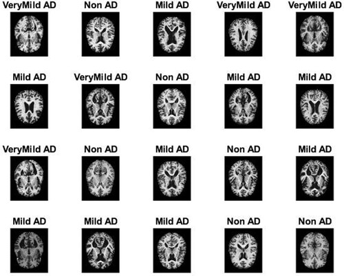
All techniques proposed in this work were evaluated on the MRI image data set of AD available on the open-source Kaggle. The data set contains 6380 MRI images divided into four classes, with three classes representing stages of the development of AD and the fourth class being “no dementia”; this is divided in the following manner: 890 images for mild dementia, 64 images for moderate dementia, 3193 images for no dementia, and 2233 images for very mild dementia. Figure 2 describes a set of images from the AD MRI data set (“Alzheimer’s Dataset (4 Class of Images) & Kaggle”, 2022).

Figure 2. Set of MRI image samples for AD.

3.2. Mri enhancement

There are numerous artifacts and noises in MRI images due to patient movement after taking MRI images. Noise also includes light reflections, different brightness of images, and other factors that affect the accuracy of diagnosis in the image processing stages. The resulting bias field is also due to the different intensity values of MRI images, ranging from black to white. Therefore, image optimisation is essential for the success of the subsequent stages and for obtaining a high-efficiency diagnostic accuracy (Budak et al., 2022). In this study, the average greyscale of all MRI images was calculated. First, the average filter was set to 6 × 6 pixels to improve the contrast of the images and reveal the soft neurons (Maqsood et al., 2019). The filter replaces each pixel in the MRI image with the average of the neighbouring 35 pixels, and the process continues until each pixel in the MRI image has been processed. Equation 1(1) $f(l)=\frac{1}{L}\sum _{i=0}^{L-1}x(l-1)$(1) describes the mechanism of action of the average filter (Ibrahim Abunadi & Senan, 2021). (1) $f(l)=\frac{1}{L}\sum _{i=0}^{L-1}x(l-1)$(1) where $f(l)$ represents the input, $x(l-1)$ represents the prior input, and L represents the number of pixels.

Second, a Laplacian filter was applied that detects the edges of soft neurons from MRI images with high accuracy. Equation 2 shows how the filter performs. (2) $\mathrm{\nabla }{}^{2}f=\frac{\mathrm{\partial }{}^{2}f}{{\mathrm{\partial }}^{2}x}+\frac{\mathrm{\partial }{}^{2}f}{{\mathrm{\partial }}^{2}y}$(2) where $\mathrm{\nabla }{}^{2}f$ refers to a differential equation of second order; and x, y refers to the locations of the matrix presented.

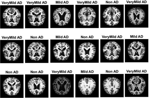
Finally, the output of the filters is combined to obtain improved high-resolution images, where the images obtained from the average filter are subtracted from the images obtained from the Laplacian filter, as indicated in Equation 3(3) $\text{output }=f(l)-\mathrm{\nabla }{}^{2}f$(3) . (3) $\text{output }=f(l)-\mathrm{\nabla }{}^{2}f$(3) Figure 3 presents a set of images for each class of the MRI data set obtained after the enhancement method.

Figure 3. Set of MRI samples after the enhancement method.

3.3. The first proposed system

3.3.1. The adoptive region growing algorithm

MRI images of AD include a large number of soft and healthy neurons. Thus, extracting features from complete MRI images will likely lead to incorrect taxonomic results. Therefore, it is necessary to separate the regions of interest from the remainder of the image for more analysis in the next stages (Ithapu et al., 2014; Yang et al., 2022). In this study, the adoptive region growing algorithm is applied; this algorithm works to group similar pixels into sub-regions. For the success of the partition process, the next conditions should be satisfied:

• ${\cup }_{i=1}^m{x}_i=x\text{where}m\text{is the regions number}$

• $x_i=1,2,\dots \dots ,M\text{ is connected}$

• $P(x_i)=\text{TRUE}\text{for }1,2,\dots \dots ,M$

• $P(x_i\cup x_j)\text{FALSE for}i\ne j\text{Where}{x}_i\text{ and }{x}_j\text{are neighboring regions}$

First, the partition process should be complete. Second, all equal pixels should be in the same sub-region, and the union of all sub-region should yield a complete image. Third, all equal pixels should be corrected, when applied to the entire image. Fourth, no two pixels are equal and belong to two various sub-regions. The algorithm works a bottom-up method, which begins with pixels to form sub-regions. The algorithm uses local information to begin creating regions. The key idea of this method is to begin with numerous different pixels as essential seeds to form regions; the number of regions begins to grow gradually to form a variety of regions; each region has similar pixels (Lazli et al., 2020). The process continues until all the pixels are completed, and each pixel is assigned to its sub-region.

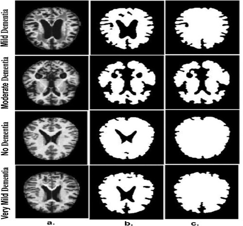
Figure 4(a) depicts a set of original images of the AD data set. Figure 4(b) depicts a set of samples of the AD data set after segmentation and identification of regions of interest (ROI). After the segmentation operations, there are holes remaining that do not belong to the ROI. Therefore, the morphological technique is applied, which receives a binary image and produces an improved binary image by filling in the holes produced after the segmentation process, as illustrated in Figure 4(c).

Figure 4. A few MRI samples for all classes of an Alzheimer’s data set a. Original image b. After the segmentation process c. After the morphology process.

It is worth noting that this technique creates the structure element, which contains a set of 3 * 3 pixels so that the structure element wraps on each location of the image and moves till to the end of the image. The method tests the template of the structure element whether it “fits” the adjacent pixels or not, while the intersection method is called “hits”. There are many operations of the morphological method such as closing, dilation, opening and erosion (Huang et al., 2022).

3.3.2. Hybrid technique to extract the features

In this section, the extraction of features is described using three algorithms – LBP, DWT, and GLCM. All the extracted features are integrated into a single feature vector (Too et al., 2021). First, the features were extracted using the LBP method in which the algorithm was set to 4 × 4 pixels. The algorithm extracted the texture of binary surfaces from MRI images by replacing each central pixel with adjacent pixels. The radius (R) parameter describes the number of pixels adjacent to each central pixel; in this study, R is 15 pixels (Karim et al., 2021). Equation 4(4) $LBP(x_c,y_c{)}_{R,P}=\sum _{p=0}^{P-1}s((g_p-g_c){.2}^p,$(4) expresses the arithmetic mechanism of the algorithm, which works to target a central pixel (g_c) and then replaces it with neighbouring pixels (g_p) in each iteration. In this method, 203 features were extracted (E. M. Senan & Jadhav, 2021). (4) $LBP(x_c,y_c{)}_{R,P}=\sum _{p=0}^{P-1}s((g_p-g_c){.2}^p,$(4) where P refers to the number of pixels and the threshold $x_c$, as in Equation (5). (5) $s(x)=\{\begin{array}{ll}0,& x<0\\ 1,& x\ge 0\end{array}$(5) Second, features were extracted using the DWT algorithm using square mirror filters; this leads to the division of input signals into two different signals based on low-pass filters and high-pass filters (Swain et al., 2020). DWT produced approximation parameters and three detailed parameters using low and high filters. The low filters produced approximate coefficients, while the high filters produced three detailed coefficients (vertical, horizontal, and diagonal). Each filter extracted three features: mean, standard deviation, and variance. Thus, the algorithm produced 12 statistical features (Sun et al., 2021).

Third, features were extracted using the GLCM method, which yields a combination of grey levels for the ROI region. The texture feature extraction by GLCM helps identify numerous areas of the ROI. The GLCM algorithm calculates texture features by distinguishing between coarse and smooth regions through pixel values. The rough region contains pixel values that are far apart, while the soft region contains pixel values that are close together. The algorithm relies on spatial information to extract features from an area of interest. It then calculates texture metrics from spatial data that specifies the connection between pixel pairs based on distance, d, and directions, θ. The distance, d, describes the distance between a pixel and its neighbour, and θ describes the directions between a pixel and its neighbouring pixels. Four values are obtained for θ – 0°, 45°, 90°, and 135°, and there is a relationship between distance d and θ. When d = 1, the angle θ between the pixel and its neighbour is vertical (θ = 0) and horizontal (θ = 90); Whereas when d = √2, the angle between the pixel and its neighbour = 45 or θ = 135 (E. M. Senan & Jadhav, 2022). This algorithm produces 13 statistical features for each image (Raghavaiah & Varadarajan, 2022).

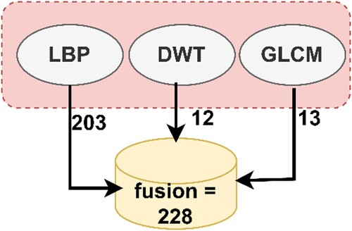
Finally, the fusion technique was used to combine the features extracted by the three algorithms to form highly efficient feature vectors. The LBP algorithm yielded 203 features, the DWT algorithm yielded 12 features, and the GLCM method yielded 13 features. Thus, the fusion method produced 228 features. Fusing the features yielded representative features for each image through which the system can distinguish each image and classify it into the appropriate class. Figure 5 presents the fusion process among the three algorithms (Liu et al., 2022).

Figure 5. Display of the fusion method among the LBP, DWT, and GLCM method.

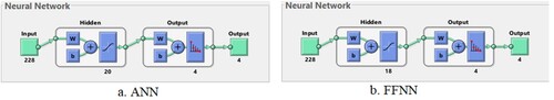
3.3.3. Ann and FFNN algorithms

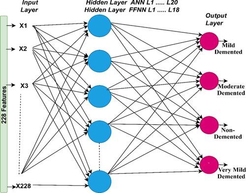
The ANN algorithm is a highly efficient neural network that comprises three layers, each containing a large number of neurons. The input layer is the first layer in the network that receives features from the feature extraction stage. The input layer consists of 228 input units in accordance with the number of features (E. Song & Li, 2021). ANN also contains numerous hidden layers; each layer has many interconnected neurons in each layer and in subsequent layers. Hidden layers solve complex problems in order to perform certain tasks (E. Senan et al., 2022). In this study, the ANN consists of 20 hidden layers while FFNN consists of 18 hidden layers to classify AD (Elhoseny et al., 2022). Several experiments were carried out for both ANN and FFNN networks with changing the number of hidden layers each time. The best performance of ANN was reached when the number of hidden layers was 20 hidden layers, while FFNN achieved the best performance when the number of hidden layers was 18 (Xu et al., 2022).

In this study, the output layer consists of four neurons – Mild Dementia, Moderate Dementia, No Dementia, and Very Mild Dementia (each neuron represents a class of the data set). The ANN algorithm analyzes and interprets complex data to perform specific tasks to recognise patterns (Z. Wang et al., 2022). Neurons are interconnected by weights, w, which represent the information transmitted from one cell to another and from one layer to another. in each iteration, the algorithm updates the weights and calculates the minimum square error (MSE) between the actual and predicted values (Munadhil et al., 2020). The algorithm continues the iterations until the lowest MSE is got between the actual y value and the predicted x value, as defined in Equation 6. (6) $\text{MSE}=\frac{1}{n}\sum _{i=1}^n(x_i-y_i{)}^2$(6) where x represents predicted values, y represents actual values, i represent a counter starting from the one, and n represents number of pixels.

The FFNN algorithm is a type of neural network that solves numerous complex tasks. Its structure is similar to ANN. In this study, the input layer contains 228 input units, and the network contains 18 hidden layers; each layer has numerous neurons interconnected by weights (w). The output layer produces four neurons same the number of classes in the AD data set. The algorithm works in the forward direction, where information is transmitted from the input layer to the output layer (El-Sappagh et al., 2020). This is called the frontal phase, which implies that the output of each neuron (weight with bias) is passed from one neuron to the other in the forward direction. The weights are updated on each iteration until an MSE is got between the actual and predicted values. The algorithm stops training when it reaches the minimum error, which is considered the best performance of the algorithm. Figure 6 describes the structures of the ANN and FFNN with all the layers and number of neurons per layer.

Figure 6. Structure of the ANN and FFNN for classifying the AD data set.

3.4. Deep learning models

Deep learning models have been used in numerous fields to perform specific tasks and solve complex problems, including the diagnosis of biomedical images. Deep learning involves a multilayered convolutional neural network (CNN) with millions of neurons interconnected by millions of connections (I Abunadi et al., 2022). Deep learning models analyze two-dimensional biomedical images and can be adapted to analyze one-dimensional and three-dimensional images (D’Angelo et al., 2021). A CNN consists of input layers for receiving inputs, output layers for displaying CNN performance, and hidden layers including convolutional layers, pooling layers, fully connected layers (FCL), and numerous auxiliary layers. The architecture of a CNN is a multilayer network in which information is forwarded and hidden layers are stacked sequentially, thereby enabling it to learn hierarchically. The essence of CNN’s work is that it obtains a multilevel representation that shifts from simple levels to more abstract and highly representative levels. The hidden layers amplify the most important representations and suppress irrelevant representations.

Convolutional layers are one of the most critical layers of CNN models that derive their name from Convolutional Neural Networks. Three parameters control how convolutional layers work: filter size, zero padding, and p-step (Qin, 2022). The filter size controls how much the filter wraps around the images at a time, and increasing the size of the filter implies more wrapping around the image. Each filter performs a specific task (Al-Khuzaie et al., 2021). One filter is concerned with the features of the colour, another with the features of the shape, another with geometric features, one that shows the edges, and so on. Each convolutional layer reveals the most complex features (J. Zhang & Tai, 2021). Zero padding is the process of lining images with zero edges to preserve the size of the original image when wrapped around the filter. The p-step is the amount of jump or the amount the filter moves around the image at a particular time. Equation 7(7) $y(t)=(x\ast f)(t)=\int x(a)f(t-a)da$(7) describes how convolution layers work and reveals that the filter f (t) is convoluted around the image x (t). (7) $y(t)=(x\ast f)(t)=\int x(a)f(t-a)da$(7) where x(t) represents the input, f(t) represents the filter, and y(t) is the output in the convolutional layer.

The ReLU layer is an auxiliary layer that follows a few convolutional layers. The ReLU layer performs a few tasks for further processing the data, as it passes the positive value and converts the negative value to zero, as described in Equation 8. (8) $\text{ReLU}(\text{x})=max(0,x)=\{\begin{array}{ll}x,& x\ge 0\\ 0,& x<0\end{array}$(8) Overfitting is one of the problems that CNN models encounter during the training phase, as convolutional layers create millions of parameters. Thus, the CNN dropout layer provides a solution to this challenge. The dropout layer passes a certain amount of information to the neurons in each iteration. In this work, the layer was set to 50%; thus, CNN models pass 50% of the information among neurons in each iteration, but this layer will double the training time (Wu et al., 2022).

Pooling layers are one of the layers of CNN models that help to reduce the massive dimensions produced by convolutional layers. Pooling layers reduce dimensions, with filters representing a group of pixels with a single pixel. There are two ways that Pooling layers work – Max and Average (S. H. Wang & Chen, 2018). The max-pooling method is a mechanism through which filters work by selecting groups of pixels and selecting max pixels from among the groups (Zhao et al., 2022). These pixel groups are represented by max pixels, as indicated in Equation 9. The average pooling method is a mechanism through which filters work by selecting certain groups of pixels. Then, the average value of the specified pixels is calculated and the number of pixels is represented by the average of the specified pixels, as indicated in Equation 10 (Dai & Wang, 2021). (9) $\begin{array}{rl}P(i;j)& =ma{x}_{m,n=1\dots .k}A[(i-1)s+m;(j-1)s+n]\end{array}$(9) (10) $\begin{array}{rl}P(i;j)& =\frac{1}{k^2}\sum _{m,n=1\dots .k}A[(i-1)s+m;(j-1)s+n]\end{array}$(10) where A refers to the number of pixels in the filter (matrix); m and n refer to the matrix dimensions, k is the matrix amplitude, and $s$ is the step (Hu et al., 2021).

The FCL is the last layer in a CNN model and is responsible for classification. This layer transforms feature maps into two dimensions (Dai & Wang, 2021). The FCL contains interconnected neurons to perform classification tasks with high accuracy. The SoftMax activation function is the last stage in CNN models that matches each image in the data set to its appropriate class, as indicated in equation 11 (B. Yang et al., 2022). In this study, SoftMax yields four classes – Mild Dementia, Moderate Dementia, No Dementia, and Very Mild Dementia. (11) $y(x_i)=\frac{\exp x_i}{{\sum }_{\text{j}=1}^{\text{n}}\exp x_j}$(11) $y(x_i)$ a value between 0 and 1.

This study focuses on two CNN models – ResNet-18 and AlexNet.

3.4.1. The resnet-18 model

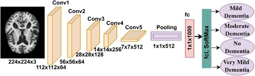
Many CNN models belong to the ResNet-xx family. In this study, the ResNet-18 model pre-trained was used, containing 18 layers distributed among five convolutional layers. Each layer has a different filter size and performs a specific task for extracting feature maps. Many ReLU layers suppress negative values in order to pass positive values and convert them to zero. The average pooling layer reduces the input dimensions (I. A. Ahmed et al., 2022). A FCL for classifying images. The SoftMax activation function produces four neurons and classifies each image of the AD data set into its appropriate class (Wenjin et al., 2022). Figure 7 describes the architecture of the ResNet-18 model, which contains a large number of layers that generate over 11.5 million parameters to classify the AD data set.

Figure 7. ResNet-18 architecture to classify the Alzheimer’s data set.

3.4.2. Alexnet model

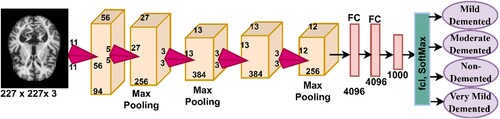
One type of CNN implemented in this study is AlexNet, which consists of 25 different layers that include convolutional, pooling, fully connected, and auxiliary layers. Moreover, five convolutional layers are included, where each layer performs a specific task for extracting feature maps. ReLU layers pass positive data and convert negative data to zero (Ying et al., 2021). Dimensionality is reduced by max pooling of three layers. In addition, two dropout layers overcome the problem of overfitting(Al-Mekhlafi & Senan, 2022 2022). To classify a data set, AlexNet has three FCLs. The SoftMax activation function produces four neurons, and each neuron represents a class for the AD data set. The network contains over 650,000 neurons interconnected by 630 million connections and produces 62 million parameters. Figure 8 describes the structure of the AlexNet network, which consists of the numerous layers that are illustrated in the figure.

Figure 8. AlexNet architecture for classifying the Alzheimer’s data set.

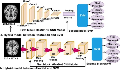
3.5. Hybrid between deep and machine learning

CNN models are among the best techniques for pattern recognition and image classification, but they require high-specification computer resources and take a long time to train the data set. This is one of the challenges facing CNN models. Therefore, techniques that are a hybrid of deep and machine learning solve these challenges (Zheng et al., 2021). These techniques consist of two parts: the first part is CNN models, and the second is the SVM algorithm (Cai et al., 2022). In the first part, CNN models extract the features. In the second part, the SVM algorithm classifies the feature extracted from the first part (Mohammed et al., 2021b). Hybrid techniques require medium-cost computer resources and do not take long to train the data set. Figure 9 describes the performance of hybrid techniques for classifying the AD data set. Figure 9(a). represents the ResNet-18 + SVM network, while Figure 9(b). represents the AlexNet + SVM network.

Figure 9. The hybrid method between deep learning and SVM algorithm a. ResNet-18 + SVM and b. AlexNet + SVM.

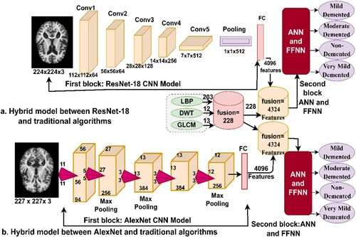
3.6. Hybrid features of deep learning and traditional algorithms

This section presents a hybrid technique for feature extraction using CNN models and traditional feature extraction algorithms, LBP, DWT, and GLCM, and then their classification by ANN and FFNN neural networks. In addition, this technique requires medium-cost computer resources and does not take long to train. The idea of this technique can be described in the following manner: First, feature maps were extracted from the two models, ResNet-18 and AlexNet, which produced 4096 features for each image in each model. Second, feature extraction was performed using the LBP, DWT, and GLCM methods; combining all three algorithms produced 228 features for each image. Third, all the features were unified into a unified data system. Fourth, all the features obtained from the CNN model and LBP, DWT, and GLCM algorithms were combined so that each feature vector stores 4324 features. Fifth, the features were fed into ANNs and FFNNs to classify them with high accuracy and efficiency. Figure 10 presents the hybrid technique, in which it is observed the features are extracted from the ResNet-18 and AlexNet models, combined with LBP, DWT, and GLCM algorithms, and then fed to the ANN and FFNN classifiers.

Figure 10. The architecture for merging the features between deep learning and traditional algorithms.

4. Experimental results

4.1. Dividing the data set

In this study, MRI images of the Alzheimer’s data set were evaluated using multimethod techniques – neural network algorithms, deep learning models, hybrid techniques between deep and machine learning, and, finally, the technique of combining features extracted by deep learning models with features extracted by the LBP, DWT, and GLCM algorithms. The data set contains 6380 MRI images distributed over four types of non-balanced classes, which are essentially three classes that represent the development stages of AD in addition to the normal fourth class. The MRI images of the data set are distributed in the following manner: 890 images of mild dementia, with a rate of 13.95%; 64 images of moderate dementia, with a rate of 1.05%; 2233 images of very mild dementia, with a rate of 35%; and the last class with 3193 images of no dementia with a rate of 50%. The AD dataset was divided for the training and validation phase with 80% and for the testing phase with 20%. Table 1 presents the division of the data set and the number of images in each stage.

Table 1. The division of the data set for AD diagnosis.

Phase	training and validation of 80%	testing of 20%
Classes	Training (80%)	validation (20%)
Mild dementia	570	142	178
Moderate dementia	41	10	13
Non-dementia	2043	511	639
Very mild dementia	1429	357	447

4.2. Metrics for evaluating the proposed systems

Four proposed methods were evaluated in this study – each method with more than one algorithm: neural networks, deep learning models, a hybrid technique between deep and machine learning, and a hybrid feature extraction technique between deep learning models and traditional algorithms (LBP, DWT, GLCM) for diagnosing AD through several metrics.

In this work, all the proposed systems were evaluated with the same measures: accuracy, precision, sensitivity, specificity, and AUC, as shown by the equations below. The information for the equations was obtained from the confusion matrix, which represents the evaluation output of systems performance. The confusion matrix includes all the perfectly classified images (TP and TN) and all the imperfectly classified images (FP and FN) (E. M. Senan et al., 2021). (12) $\begin{array}{rl}\text{Accuracy}& =\frac{\text{TN}+\text{TP}}{\text{TN}+\text{TP}+\text{FN}+\text{FP}}\ast 100\mathrm{\%}\end{array}$(12) (13) $\begin{array}{rl}\text{Precision}& =\frac{\text{TP}}{\text{TP}+\text{FP}}\ast 100\mathrm{\%}\end{array}$(13) (14) $\begin{array}{rl}\text{Sensitivity}& =\frac{\text{TP}}{\text{TP}+\text{FN}}\ast 100\mathrm{\%}\end{array}$(14) (15) $\begin{array}{rl}\text{Specificity}& =\frac{\text{TN}}{\text{TN}+\text{FP}}\ast 100\end{array}$(15) (16) $\begin{array}{rl}\text{AUC }& =\frac{\text{True Positive Rate}}{\text{False Positive Rate}}=\frac{\text{Sensitivity}}{\text{Specificity}}\end{array}$(16)

TP is the number of MRI images which classified perfectly as AD. TN is the number of MRI images which classified perfectly as healthy samples. FP is the number of MRI images of normal samples but classified as AD. FN is the number of MRI images of AD that are classified as normal.

4.3 Results of the neural networks

This section explains the performance of the ANN and FFNN neural networks for diagnosing the AD data set. ANN and FFNN depend on the accuracy and efficiency of the features extracted from the previous stage. In this study, the ANN and FFNN were fed with the features extracted in a hybrid method by LBP, DWT, and GLCM algorithms. Therefore, the classification stage depends on the accuracy of the previous stages in image processing. Figure 11 describes the training of the AD data set by ANN and FFNN. It indicates that the input layer contains 228 input units and 20 hidden layers of the ANN, while the FFNN achieved the best performance with 18 hidden layers. It is also evident that there is an output layer, which contains four neurons based on the number of classes of the data set, where each neuron represents one of the classes in the data set.

Figure 11. Training of neural networks to evaluate the AD data set.

There are many tools for evaluating the performance of ANN and FFNN, which are described here.

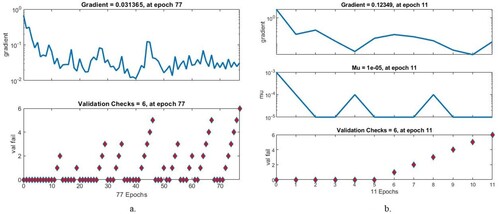
4.3.1. Gradient and validation checks.

In this study, the neural networks ANN and FFNN were evaluated using the gradient and validation checks on the AD dataset. Algorithms set both gradient and validation checks when networks attain minimum error. Figure 12 describes the performance of the ANN and FFNN when evaluating the AD data set. It must be noted that when ANN attains the minimum error, the ANN has a gradient value of 0.031365 and a validation check of 6 at epoch 77. When the FFNN attains the minimum error, the FFNN has a gradient value of 0.12349 and a validation check of 6 at epoch 11.

Figure 12. Display Gradient for evaluating neural network performance for the AD dataset a. ANN b. FFNN.

4.3.2. Best validation performance

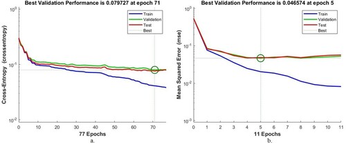
Cross-entropy or mean square error is an assessment tool for ANNs and FFNNs of the AD data set. Cross-entropy evaluates the performance of neural networks during all phases and passes through several epochs. The algorithms obtain the mean square error in each epoch, which measures the minimum error between the expected and actual values. The algorithm worked until it reached the best performance, when it obtained the least square error. Figure 13 describes the evaluation of the AD data set by ANNs and FFNNs during all stages. The blue colour represents the network performance during the training phase, the green colour during the validation phase, and the red colour during the testing phase. The ANN algorithm attained the minimum error at the best validation result, with a value of 0.079727 at epoch 71. The FFNN attained the minimum error at the best validation result, with a value of 0.046574 at epoch 5.

Figure 13. Display of the validation performance of neural networks on the AD data set a. ANN b. FFNN.

4.3.3. Error histogram

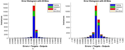
An error histogram is a benchmarking tool for evaluating the ANN and FFNN on the AD data set that measures the error between target and output values. The error histogram evaluates the performance of neural networks during all phases (training, validation, and testing). In each phase, the algorithm is evaluated with a histogram bin. The histogram bin represents the training phase in blue, the testing phase in red, and the validation phase in green colour. The orange colour represents the best network performance, which implies that the error between the target and output values is zero. Figure 14 indicates the performance of the ANN and FFNN in evaluating the AD data set by error histogram. It is noticed that the ANN algorithm achieved the best result when it passed through 20 bins between the values – 0.9486 and 0.9486. In contrast, FFNN achieved the best result when it passed through 20 bins of values between – 1.19 and 1.229.

Figure 14. Display error histogram for evaluating neural network performance for an AD data set a. ANN b. FFNN.

4.3.4. Receiver operating characteristic (ROC)

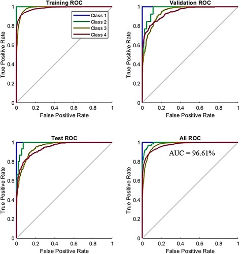
ROC is one of the essential tools for measuring the performance of an ANN algorithm for evaluating the AD data set; it measures both true positive and false negative samples and is called the AUC. True positive samples are represented on the y-axis, while false negative samples are on the x-axis. The ROC evaluates the performance of the ANN during all phases. At each phase, the ANN is evaluated by dividing the true-positive sampling rate by the false – positive sampling rate. ANN performs best when the curve approached from the left corner. Figure 15 describes the performance of ANN for evaluating the AD data set at all stages. The four colours used in the figure represent all classes in the data set. ANN reached a total AUC of 96.61% for all phases and classes in the data set.

Figure 15. Display ANN performance for evaluating neural network performance for an AD data set.

4.3.5. Confusion matrix

This section explains the results of the ANN and FFNN for evaluating the AD data set through the confusion matrix. A confusion matrix is a form that resembles a quadrilateral matrix. Each row and column represent one of the classes (disease) of the data set. In this study, the ANN and FFNN produced a confusion matrix of four rows and four columns, which contains all samples of a correctly classified AD data set, called TP, that is represented by the main diagonal of the matrix. The remainder of the confusion matrix cells represent incorrectly classified images called FP and FN. Figure 16 describes the confusion matrix for the ANN and FFNN. Class 1 represents the Mild Dementia stage, Class 2 represents the Moderate Dementia stage, Class 3 represents the No Dementia normal state, and Class 4 represents the Mild Dementia stage. It is evident that the ANN algorithm achieved an accuracy of 98.7%, while the FFNN achieved an accuracy of 98.9%. Therefore, the FFNN outperformed ANN in diagnosing the AD data set.

Figure 16. Confusion matrix for the Alzheimer’s data set evaluation using a. ANN b. FFNN.

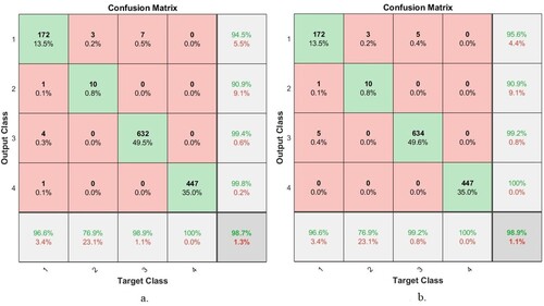
Thus, the FFNN and ANN algorithms based on the hybrid features contributed to diagnosing the stages of AD progression. Table 2 presents the evaluation results of the two algorithms. ANN obtained an accuracy of 98.7%, a precision of 98.5%, a sensitivity of 98%, a specificity of 99.56%, and an AUC of 96.61%. In comparison, FFNN achieved an accuracy of 98.9%, precision of 96.5%, sensitivity of 96.25%, specificity of 99.5%, and AUC of 97.69%.

Table 2. Evaluation of the AD Dataset by ANN and FFNN.

Measure	ANN	FFNN
Accuracy %	98.7	98.9
Precision %	98.5	96.5
Sensitivity %	98	96.25
Specificity %	99.56	99.5
AUC %	96.61	97.69

Figure 16 shows the number of correctly classified and incorrectly classified samples for Figure 16(a): Class 1 (Mild Dementia) 172 out of 178 images were correctly classified, while 6 images were incorrectly classified. Class 2 (Moderate Dementia) 10 of the 13 images are classified correctly, while 3 are classified incorrectly. For Class 3 (No Dementia), 632 of the 639 images were correctly classified, while 7 were incorrectly classified. For Class 4 (Mild Dementia), 447 of the 447 images are correctly classified, while there are no failed samples. Whereas for FFNN, Figure 16(b) is as follows: Class 1 (Mild Dementia) 172 out of 178 images are classified correctly while 6 images are incorrectly classified. Class 2 (Moderate Dementia) 10 of the 13 images are classified correctly, while 3 are classified incorrectly. For Class 3 (No Dementia), 634 of the 639 images were correctly classified, while 7 were incorrectly classified. For Class 4 (Mild Dementia), 447 of the 447 images are correctly classified, while there are no failed samples.

4.4. Experimental results of deep learning

This section presents the experimental results achieved by the ResNet-18 and AlexNet models to track the progression of AD. Pre-trained models have been trained more than a million times to create more than a thousand classes. Nevertheless, unfortunately, the huge data set does not contain images for most diseases. Therefore, it is possible to perform new tasks by transferring the experience of these pre-trained models to a new data set. In this study, the knowledge of these models was transferred and the parameters were set at the best performance level for evaluating and tracking the stages of AD progression.

Deep learning models face the following challenges: they require a huge data set to avoid overfitting during the training phase. This challenge can be addressed using the augmentation method of the data available in deep learning models. This method also balances the data set by artificially increasing the number of images during the training phase. The images of the minority classes are increased by a greater number than that of the majority classes. The data augmentation method also leads to an increase in the number of images on account of numerous operations, such as rotating in several angles, shifting, cropping, flipping, etc. Table 3 presents the number of images in the data set before and after the augmentation method, the images were artificially increased during the training phase.

Table 3. Image augmentation in the data set by the data augmentation method.

Phase	Training phase
Stages of disease progression	Mild dementia	Moderate dementia	Non-dementia	Very mild dementia
Before augmentation	570	41	2043	1429
After augmentation	2,280	1,230	2,043	2,858

It is evident from the table that the images increased differently from one class to another. There was an increase of four images for each image in the Mild Dementia stage; an increase of 30 images for each image in the Moderate Dementia class; and an increase of two images for each image in the Very Mild Dementia stage. The data augmentation method was not applied to the No Dementia category, as it contains a sufficient number of images.

The data set has undergone numerous experiments with the ResNet-18 and AlexNet models, and in each experiment, the training options were changed until a high-efficiency performance was obtained. The models were reset until the best performance was reached for the two models, as indicated in Table 4.

Table 4. Training options ResNet-18 and AlexNet.

Options	ResNet-18	AlexNet
Training Options	adam	adam
Mini Batch Size	15	130
Max Epochs	6	10
Initial Learn Rate	0.0003	0.0001
Validation Frequency	5	50
Training time (min)	166 min 45 sec	25 min 53 sec
Execution Environment	GPU	GPU

After adjusting the training options and parameters of the ResNet-18 and AlexNet models, superior results were obtained in detecting the stages of AD progression. Table 5 presents the results achieved by the deep learning models, where it is noted that the AlexNet model is superior to the ResNet-18 model. The ResNet-18 model yielded an accuracy of 93.9%, precision of 95.5%, sensitivity of 94.75%, specificity of 96%, and AUC of 99.48%. In comparison, the AlexNet model achieved an accuracy of 94.6%, precision of 94.25%, sensitivity of 89.75%, specificity of 98%, and AUC of 99.9%.

Table 5. Performance of deep learning models for identifying AD progression stages.

Measure	ResNet-18	AlexNet
Accuracy %	93.9	94.6
Precision %	95.5	94.25
Sensitivity %	94.75	89.75
Specificity %	96	98
AUC %	99.48	99.9

Figure 17 shows the number of correctly classified and incorrectly classified samples for Figure 17(a): In the Mild Dementia class, 167 out of 178 images were correctly classified, while 11 images were incorrectly classified. In the Moderate Dementia class, 13 of the 13 images are classified correctly, while there are no failed samples. For the No Dementia class, 633 of the 639 images were correctly classified, while 6 were incorrectly classified. For the Mild Dementia class, 386 of the 447 images are correctly classified, while 61 were incorrectly classified. Whereas for AlexNet, Figure 17(b) is as follows: In the Mild Dementia class, 164 out of 178 images were correctly classified, while 14 images were incorrectly classified. In the Moderate Dementia class, 10 of the 13 images are classified correctly, while 3 images were incorrectly classified. For the No Dementia class, 609 of the 639 images were correctly classified, while 30 were incorrectly classified. For the Mild Dementia class, 425 of the 447 images are correctly classified, while 22 were incorrectly classified.

Figure 17. Confusion matrix for performing deep learning models to detect AD progression a. ResNet-18 b. AlexNet.

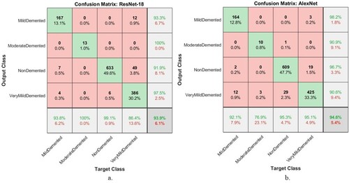
ResNet-18 and AlexNet models produced a confusion matrix, a tool for evaluating the progression of AD, as shown in Figure 17. It is evident that AlexNet is superior to ResNet-18. The ResNet-18 model achieved accuracy for diagnosing Mild Dementia of 93.8%, Moderate Dementia of 100%, No Dementia of 99.1%, and Very Mild Dementia of 86.4%. In comparison, the AlexNet model achieved accuracy for diagnosing Mild Dementia of 92.1%, Moderate Dementia of 76.9%, No Dementia of 95.3%, and Very Mild Dementia of 95.1%.

4.5. Experimental results of the hybrid model of the deep and machine learning models

This section reviews experimental results of the hybrid model of the deep and machine learning models for early detection of AD progression. This hybrid technique is based on extracting feature maps using ResNet-18 and AlexNet models and feeding deep feature maps to SVM. These techniques have achieved superior results in classifying the Alzheimer’s stage data set with high accuracy and efficiency. The hybrid technique has reached results that surpass deep learning models. Table 6 summarises the performance of the hybrid ResNet-18 + SVM and AlexNet + SVM techniques for early detection of AD stages. ResNet-18 + SVM achieved an accuracy of 97.9%, precision of 98.5%, sensitivity of 85.5%, specificity of 99%, and AUC of 97.89%. In comparison, the AlexNet + SVM technique achieved an accuracy of 98.5%, precision of 99%, sensitivity of 86.75%, specificity of 99.25%, and AUC of 98.51%. The ResNet-18 + SVM technique slightly outperforms the AlexNet + SVM hybrid technique.

Table 6. Performance of hybrid models for early detection of progression AD.

Measure	ResNet-18 + SVM	AlexNet + SVM
Accuracy %	97.9	98.5
Precision %	98.5	99
Sensitivity %	85.5	86.75
Specificity %	99	99.25
AUC %	97.89	98.51

Figure 18 shows the number of samples classified correctly and incorrectly by hybrid techniques. The Figure 18(a) shows all samples classified as follows: In the Mild Dementia class, 157 out of 178 images were correctly classified, while 21 images were incorrectly classified. In the Moderate Dementia class, 7 of the 13 images are classified correctly, while 6 were incorrectly classified. For the No Dementia class, 639 of the 639 images were correctly classified, while there are no failed samples. For the Mild Dementia class, 447 of the 447 images are correctly classified, while there are no failed samples.

Figure 18. Performance of hybrid techniques for evaluating a data set of AD during its development stages a. ResNet-18 + SVM b. AlexNet + SVM.

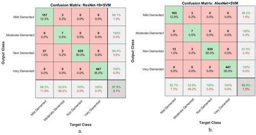
Whereas for AlexNet + SVM, Figure 18(b) shows all samples classified as follows: In the Mild Dementia class, 165 out of 178 images were correctly classified, while 13 images were incorrectly classified. In the Moderate Dementia class, 7 of the 13 images are classified correctly, while 6 images were incorrectly classified. For the No Dementia class, 639 of the 639 images were correctly classified, while there are no failed samples. For the Mild Dementia class, 447 of the 447 images are correctly classified, while there are no failed samples.

Hybrid techniques have achieved superior results in detecting the progression of AD. Figure 18 presents the confusion matrix produced by ResNet-18 + SVM and AlexNet + SVM hybrid models. The ResNet-18 + SVM model achieved accuracy for diagnosing Mild Dementia of 88.2%, Moderate Dementia of 53.8%, No Dementia of 100%, and Very Mild Dementia of 100%. On the other hand, the AlexNet + SVM model achieved accuracy for diagnosing Mild Dementia of 92.7%, Moderate Dementia of 53.8%, No Dementia of 100%, and Very Mild Dementia of 100%.

4.6. Experimental results of the hybrid features of CNN with traditional algorithms.

In this section, the performance of hybrid techniques is presented based on the hybrid features of deep learning models and LBP, DWT, and GLCM algorithms and their classification by ANN and FFNN neural networks. These techniques are characterised by their rapid training of data sets and their highly efficient performance in the early detection of AD progression stages.

Table 7 summarises the evaluation performance of ANN and FFNN for diagnosing the AD data set based on feature maps from ResNet-18 and AlexNet models and combining them with the hybrid features from LBP, DWT and GLCM algorithms. Both ANN and FFNN algorithms were fed with the same hybrid features; FFNN achieved better performance than ANN. Four experimental results are presented in this section, as shown in the table, two experiments with ANN and two experiments with FFNN: First, the ANN network, when fed with the hybrid features extracted by ResNet-18 with features of the LBP, DWT, and GLCM algorithms, it achieved an accuracy of 99.6%, precision of 99.61%, sensitivity of 99.89%, specificity of 99.61%, and AUC of 99.75%. In comparison, when ANN was fed with the hybrid features extracted by AlexNet with features of LBP, DWT, and GLCM algorithms, it achieved an accuracy of 99.7%, precision of 99.08%, sensitivity of 99.95%, specificity of 99.09%, and AUC of 99.51%. Second, when the FFNN was fed with the hybrid features extracted by ResNet-18 with features of the LBP, DWT, and GLCM algorithms, it yielded an accuracy of 99.8%, precision of 99.9%, sensitivity of 99.75%, specificity of 100%, and AUC of 99.94%. In comparison, when the FFNN was fed with the hybrid features extracted by AlexNet with features of LBP, DWT, and GLCM algorithms, it obtained an accuracy of 99.5%, precision of 98.55%, sensitivity of 99.85%, specificity of 98.57%, and AUC of 99.21%.

Table 7. Performance of neural networks with fusion features for early detection of AD progression.

Classifiers	ANN		FFNN
Hybrid Features	ResNet-18 map feature +  (LBP, DWT, and GLCM)	AlexNet map feature +  (LBP, DWT, and GLCM)	ResNet-18 map feature +  (LBP, DWT, and GLCM)	AlexNet map feature +  (LBP, DWT, and GLCM)
Accuracy %	99.6	99.7	99.8	99.5
Precision %	99.61	99.08	99.9	98.55
Sensitivity %	99.89	99.95	99.75	99.85
Specificity %	99.61	99.09	100	98.57
AUC %	99.75	99.51	99.94	99.21

ANN and FFNN achieved superior results in the early detection of AD progression. In Figure 19, the confusion matrix is produced by the ANN network based on the fusion of features between the ResNet-18 model and the LBP, DWT, and GLCM algorithms, as presented in Figure 19(a); and the hybrid features between the AlexNet model and the LBP, DWT, and GLCM algorithms, as presented in Figure 19(b). As depicted in Figure 19(a), the ANN achieved accuracy for diagnosing Mild Dementia of 98.9%, Moderate Dementia of 92.3%, No Dementia of 99.8%, and Very Mild Dementia of 99.8%. While the ANN presented in Figure 19(b) achieved accuracy for diagnosing Mild Dementia of 99.4%, Moderate Dementia of 92.3%, Non-Dementia of 100%, and Very Mild Dementia of 99.6%.

Figure 19. Confusion Matrix of ANN based on fusion features a. ResNet-18 with traditional methods and b. AlexNet with traditional algorithms.

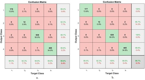
Figure 19 shows the number of correctly classified and incorrectly classified samples for Figure 19(a): Class 1 (Mild Dementia) 176 out of 178 images were correctly classified, while 2 images were incorrectly classified. Class 2 (Moderate Dementia) 12 of the 13 images are classified correctly, while one image was classified incorrectly. For Class 3 (No Dementia), 638 of the 639 images were correctly classified, while one image was incorrectly classified. For Class 4 (Mild Dementia), 446 of the 447 images are correctly classified, while one image was incorrectly classified. Whereas for Figure 19(b) is as follows: Class 1 (Mild Dementia) 177 out of 178 images are classified correctly while one image was incorrectly classified. Class 2 (Moderate Dementia) 12 of the 13 images are classified correctly, while one image was classified incorrectly. For Class 3 (No Dementia), 639 of the 639 images were correctly classified, while there are no failed samples. For Class 4 (Mild Dementia), 445 of the 447 images are correctly classified, while two images were classified incorrectly.

Figure 20 presents the performance of the FFNN classifier for detecting AD progression stages based on the combined features between the ResNet-18 model and the LBP, DWT, and GLCM algorithms, as depicted in Figure 20(a); and the combined features between the AlexNet model and the LBP, DWT, and GLCM algorithms, as illustrated in Figure 20(b). The FFNN classifier depicted in Figure 20(a). yielded accuracy for diagnosing Mild Dementia of 99.4%, Moderate Dementia of 100%, Non-Dementia of 99.7%, and Very Mild Dementia of 100%. While the FFNN presented in Figure 20(b). achieved accuracy for diagnosing Mild Dementia of 99.4%, Moderate Dementia of 84.6%, Non-Dementia of 100%, and Very Mild Dementia of 99.3%.

Figure 20. Confusion Matrix of FFNN based on combined features a. ResNet-18 with traditional methods and b. AlexNet with traditional algorithms.

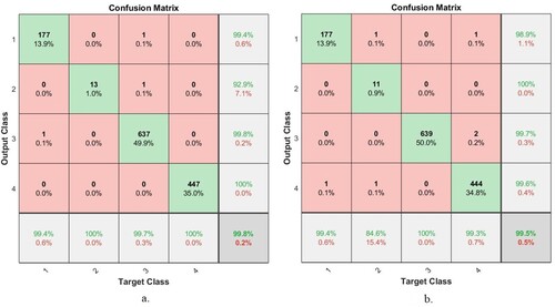
Figure 20 shows the number of correctly classified and incorrectly classified samples for Figure 20(a): Class 1 (Mild Dementia) 177 out of 178 images were correctly classified, while one image was incorrectly classified. Class 2 (Moderate Dementia) 13 of the 13 images are classified correctly, while there are no failed samples. For Class 3 (No Dementia), 637 of the 639 images were correctly classified, while two images were classified incorrectly. For Class 4 (Mild Dementia), 447 of the 447 images are correctly classified, while there are no failed samples. Whereas for Figure 20(b) is as follows: Class 1 (Mild Dementia) 177 out of 178 images are classified correctly while one image was incorrectly classified. Class 2 (Moderate Dementia) 11 of the 13 images are classified correctly, while two images were classified incorrectly. For Class 3 (No Dementia), 639 of the 639 images were correctly classified, while there are no failed samples. For Class 4 (Mild Dementia), 444 of the 447 images are correctly classified, while three images were classified incorrectly.

5. Discussion and comparison of the proposed systems with previous studies

This study presented four proposed systems; each proposed system has more than one system, and the methodology and materials used in each method were varied. This study aimed to diagnose MRI images for early detection of AD development stages. The images were enhanced with the same filters for all the proposed systems. Due to the lack of sufficient images to train the models, the data augmentation method was applied.

In this section, a discussion of all the proposed systems is presented: The first proposed system is neural networks (ANN and FFNN) based on the hybrid features extracted by the LBP, DWT, and GLCM methods. The second system is proposed by the ResNet-18 and AlexNet models based on adjusting the training options at the best performance. The third proposed system is to apply a hybrid method of deep learning to extract feature maps and then classify them using the SVM algorithm; these techniques are called ResNet-18 + SVM and AlexNet + SVM. The fourth proposed system uses ANN and FFNN based on features extracted by deep learning models and LBP, DWT, and GLCM algorithms.

The first proposed system classified the AD data set based on the features extracted from three algorithms combined together, thus feeding the ANN and FFNN with 228 representative features. The system reached an overall accuracy of 98.7% and 98.9% for ANN and FFNN, respectively. The second proposed system is ResNet-18 and AlexNet models based on feature map extraction. The system reached an overall accuracy of 93.9% and 94.6% for both ResNet-18 and AlexNet, respectively. The third proposed system, representing one of our main contributions in this study, is one where the last layers are removed from the ResNet-18 and AlexNet models and replaced by the SVM algorithm. Thus, this hybrid technique is made up of two parts: the first part is deep learning models for extracting feature maps, and the second part is SVM for classifying feature maps. This technique achieved an overall accuracy of 97.9% and 98.5% for both ResNet-18 + SVM and AlexNet + SVM, respectively. The fourth proposed system uses ANN and FFNN to classify the extracted AD data set in a hybrid of ResNet-18 and AlexNet models and LBP, DWT, and GLCM algorithms; this system represents one of our main contributions in this study. The ANN and FFNN were fed with 4324 features for each image. The system achieved superior results compared to the other proposed methods. When fed to the ANN with hybrid features by ResNet-18 and the LBP, DWT, and GLCM algorithms, it achieved an accuracy of 99.6%. When fed with hybrid features by AlexNet and LBP, DWT, and GLCM algorithms, it achieved an accuracy of 99.7%. Further, when FFNN is fed with hybrid features using ResNet-18 and LBP, DWT, and GLCM algorithms, it achieved an accuracy of 99.8%. On the other hand, when fed with hybrid features by AlexNet and LBP, DWT, and GLCM algorithms, it achieved an accuracy of 99.5%.

Table 8 shows the performance of all the systems proposed in this study for classifying MRI images for early detection of AD progression. The table summarises the performance of all systems for the diagnosis of each stage of AD. First, the ANN, and FFNN based on the features of ResNet-18+ (LBP, DWT and GLCM) achieved the best performance for Mild dementia diagnosis by 99.4%. Second, the ResNet-18 and FFNN based on the features of ResNet-18+ (LBP, DWT and GLCM) achieved the best moderate dementia performance of 100%. Third, both the proposed third (Hybrid method) and fourth (Hybrid features) systems achieved the best performance for non-dementia diagnosis by 100%. Fourth, both the proposed third (Hybrid method) and fourth (Hybrid features) systems achieved the best performance for diagnosing very mild dementia by 100%.

Table 8. Performance of all proposed systems for early detection of Alzheimer’s development stages.

Diseases	Mild dementia	Moderate dementia	No dementia	Very mild dementia	Accuracy %
Neural Networks	ANN	96.6	76.9	98.9	100	98.7
	FFNN	96.6	76.9	99.2	100	98.9
Deep learning	ResNet-18	93.8	100	99.1	86.4	93.9
	AlexNet	92.1	76.9	95.3	95.1	94.6
Hybrid	ResNet-18 + SVM	88.2	53.8	100	100	97.9
	AlexNet + SVM	92.7	53.8	100	100	98.5
Hybrid features	ANN	ResNet-18 +  (LPB, DWT, and GLCM)	98.9	92.3	99.8	99.8	99.6
		AlexNet +  (LPB, DWT, and GLCM)	99.4	92.3	100	99.6	99.7
	FFNN	ResNet-18 +  (LPB, DWT, and GLCM)	99.4	100	99.7	100	99.8
		AlexNet +  (LPB, DWT, and GLCM)	99.4	84.6	100	99.3	99.5

Figure 21 displays the performance of all proposed systems for classifying MRI images for early detection of AD progression in graphic form.

Figure 21. Proposed systems for classifying each stage of AD in graphic form.

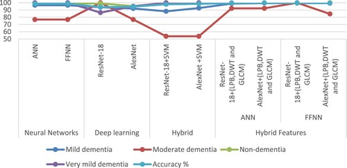
Table 9 and Figure 22 describes the evaluation results of a set of previous studies related to the diagnosis of AD and their comparison with the results of the proposed systems in this study. It is noted that our systems achieved promising results compared to previous studies. The previous systems achieved accuracy ranging from 67.7% and 93.18%, while our system achieved an accuracy of 99.8%. The previous systems achieved an allergy ranging from 68% and 93%, while our system achieved a sensitivity of 99.75%. The previous systems achieved a specificity ranging from 67.25% and 90.03%, while our system achieved a specificity of 100%.

Figure 22. Comparison of the performance of the systems with the previous systems.

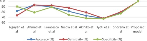
Table 9. Comparison of the performance of the systems with previous studies.

Previous research	Accuracy (%)	Sensitivity (%)	Specificity (%)
(Duc et al., 2020)	81.71	73.39	90.03
(Salehi et al., 2022)	93.18	93	79
(Morabito et al., 2017)	89	92	89
(Amoroso et al., 2022)	81	87.5	74.5
(Wada et al., 2022)	73	79	68
(Islam & Zhang, 2018 2022)	67.7	68	67.25
(Janelidze et al., 2022)	78.5	80	77
Proposed model	99.8	99.75	100

One of the most important limitations that we faced was the lack of images in the data set, especially since deep learning models need a huge data set to train the models. This limitation was overcome by applying the data augmentation method to artificially generate images from the same data set. Also, the unbalanced data set is one of the limitations that we faced because the accuracy tends to the majority classes. This challenge was addressed by a data augmentation method that increases the images of the minority classes more than the majority classes.

The novelty of this study is to extract the deep features by deep learning models and combine them with the features of texture, geometric, and shape extracted by LBP, DWT, and GLCM algorithms. The fusion method achieved promising results in the early detection of AD stages.

The reason we need to apply the fourth approach is that soft brain cells are difficult to distinguish from healthy brain cells, especially in the first stage. Handcrafted features that represent features of texture, geometry, and shape are important for the representation of MRI images, but they do not achieve satisfactory accuracy as shown in the first proposed approach. Also, the deep features extracted by CNN models do not achieve satisfactory accuracy as shown in the second proposed approach. Thus, hybrid feature extraction between CNN models and their combination with texture, geometric and shape features called handcrafted features extracted by LBP, DWT and GLCM methods result in a mixture of features stored in two feature matrices, which represents all MRI images of the Alzheimer’s dataset with high fidelity. The two feature matrices are fed into the ANN and FFNN networks for fast training and diagnosis high accuracy.

6. Conclusion and future research

Early and effective diagnosis of AD progression is essential to receive appropriate treatment to stop its progression and to care for patients. In this study, a systematic review of neural networks, deep learning, machine and hybrid techniques to diagnose MRI images for early detection of AD progression is presented. The four proposed methods are explained, each method with more than one model, in the following manner: First, MRI images of AD were classified using neural networks (ANN and FFNN) based on the features extracted in a hybrid manner using three algorithms: LBP, DWT, and GLCM. This method achieved superior results in tracking the progression of AD, achieving an overall accuracy of 98.7% and 98.9% for both ANN and FFNN, respectively. Second, deep learning models (ResNet-18 and AlexNet) were used based on extracting deep features and classifying them with high accuracy. The deep learning models found an overall accuracy of 93.9% and 94.6% for both ResNet-18 and AlexNet, respectively. Third, the hybrid technique was applied based on two blocks: The first block is the ResNet-18 and AlexNet models to extract deep feature maps. The second block is SVM to classify feature maps extracted from the first block. This hybrid technique achieved promising results in tracking the progression of AD, as it reached an overall accuracy of 97.9% and 98.5% for both ResNet-18 + SVM and AlexNet + SVM, respectively. Fourth, the AD data set was classified by two neural networks (ANN and FFNN) based on hybrid features extracted by deep learning models (ResNet-18 and AlexNet) and traditional algorithms (LBP, DWT, and GLCM). This method achieved superior results in the early diagnosis of AD. The ANN has an overall accuracy of 99.6% with the hybrid features between the ResNet-18 model with LBP, DWT, and GLCM algorithms, while the same network achieved an overall accuracy of 99.7% with the hybrid features between the AlexNet model with LBP, DWT, and GLCM algorithms. The FFNN reached an overall accuracy of 99.8% with the hybrid features between ResNet-18 model with the LBP, DWT, and GLCM algorithms; the same network reached an overall accuracy of 99.5% with the hybrid advantages of the AlexNet model with LBP, DWT, and GLCM algorithms.

Since deep learning models require a huge data set to avoid the overfitting problem, the limitations that were faced are the small number of images of AD, which was overcome by the data augmentation method that artificially increases the number of images from the same data set.

Future research could use several machine learning classifiers to classify the features extracted in a hybrid manner by CNN models and traditional algorithms.

Acknowledgments

The author would like to thank Prince Sultan University for the support provided to enable publishing this work.

Disclosure statement

No potential conflict of interest was reported by the author(s).

Data availability

The performance of the proposed systems in this study was supported by the publicly available AD data set via the following link: https://www.kaggle.com/tourist55/alzheimers-dataset-4-class-of-images.

References

- Abunadi, I, Albraikan, A. A., Alzahrani, J. S., & Eltahir, M. M., & Healthcare, and undefined 2022. (2022). An automated glowworm swarm optimization with an inception-based deep convolutional neural network for COVID-19 diagnosis and classification. Mdpi.Com. https://www.mdpi.com/1579912
- Abunadi, I., & Senan, E. M. (2021). Deep learning and machine learning techniques of diagnosis dermoscopy images for early detection of skin diseases. Electronics 2021, 10(24), 3158. Multidisciplinary Digital Publishing Institute: 3158. doi:10.3390/ELECTRONICS10243158
- Ahmed, I. A., Senan, E. M., Rassem, T. H., Ali, M. A. H., Ahmad Shatnawi, H. S., Alwazer, S. M., & Alshahrani, M. (2022). Eye tracking-based diagnosis and early detection of autism spectrum disorder using machine learning and deep learning techniques. Electronics 2022, 11(4), 530. Multidisciplinary Digital Publishing Institute: 530. doi:10.3390/ELECTRONICS11040530.
- Ahmed, O. b., Mizotin, M., Benois-Pineau, J., Allard, M., Catheline, G., Amar, B., & Allard, M. (2015). Alzheimer’s disease diagnosis on structural MR images using circular harmonic functions descriptors on hippocampus and posterior cingulate cortex. Computerized Medical Imaging and Graphics, 44, 13–25. doi:10.1016/j.compmedimag.2015.04.007
- Al-Khuzaie, F. E. K., Bayat, O., & Duru, A. D. (2021). Diagnosis of Alzheimer disease using 2D MRI slices by convolutional neural network. Applied Bionics and Biomechanics, 2021. Hindawi Limited. doi:10.1155/2021/6690539.
- Al-Mekhlafi, Z. G., Senan, E. M., & Computers, and undefined 2022. (2022). Deep learning and machine learning for early detection of stroke and haemorrhage. Eprints.Bournemouth.Ac.Uk. http://eprints.bournemouth.ac.uk/36721/
- Altinkaya, E., Polat, K., Barakli, B., & Journal of the Institute of Electronics, and undefined 2020. (2019). Detection of Alzheimer’s disease and dementia states based on deep learning from MRI images: A comprehensive review. Iecscience.Org, 1, 39–53. doi:10.33969/JIEC.2019.11005.
- “Alzheimer’s Dataset (4 Class of Images) | Kaggle”. 2022. https://www.kaggle.com/tourist55/alzheimers-dataset-4-class-of-images
- Amoroso, N., Diacono, D., Fanizzi, A., La Rocca, M., & Journal of neuroscience, and undefined 2018. (2022). Deep learning reveals alzheimer’s disease onset in MCI subjects: Results from an international challenge. Elsevier. https://www.sciencedirect.com/science/article/pii/S0165027017304296
- Ballarini, T., van Lent, D. M., Brunner, J., Schröder, A., Wolfsgruber, S., Altenstein, S., Brosseron, F., et al. (2021). Mediterranean diet, Alzheimer disease biomarkers, and brain atrophy in old age. Neurology, 96(24), e2920–e2932. Wolters Kluwer Health, Inc. on behalf of the American Academy of Neurology. doi:10.1212/WNL.0000000000012067
- Bernal-Rusiel, J. L., Reuter, M., Greve, D. N., Fischl, B., & Neuroimage, and undefined 2013. (2022). Spatiotemporal linear mixed effects modeling for the mass-univariate analysis of longitudinal neuroimage data. Elsevier. https://www.sciencedirect.com/science/article/pii/S1053811913005430
- Budak, Ü., Cömert, Z., Rashid, Z. N., Şengür, A., & Applied Soft Computing, and undefined 2019. (2022). Computer-aided diagnosis system combining FCN and Bi-LSTM model for efficient breast cancer detection from histopathological images. Elsevier. https://www.sciencedirect.com/science/article/pii/S1568494619305460
- Cai, S., Han, D., Yin, X., Li, D., & Chang, C. C. (2022). A hybrid parallel deep learning model for efficient intrusion detection based on metric learning. Taylor & Francis 34(1), 551–577. doi:10.1080/09540091.2021.2024509.
- Dai, Y., & Wang, T. (2021). Prediction of customer engagement behaviour response to marketing posts based on machine learning. Taylor & Francis 33(4), 891–910. doi:10.1080/09540091.2021.1912710.
- D’Angelo, G., Palmieri, F., Robustelli, A., & Castiglione, A. (2021). Effective classification of android malware families through dynamic features and neural networks. Taylor & Francis: 33(3), 786–801. doi:10.1080/09540091.2021.1889977.
- Duc, N. T., Ryu, S., Qureshi, M. N. I., Choi, M., Lee, K. H., & Lee, B. (2020). 3D-Deep learning based automatic diagnosis of Alzheimer’s disease with joint MMSE prediction using resting-state FMRI. Neuroinformatics, Springer: 18(1), 71–86. doi:10.1007/s12021-019-09419-w
- Ebrahimi-Ghahnavieh, A, Luo, S., & 2019 IEEE International, and undefined 2019. (2022). Transfer learning for Alzheimer’s disease detection on MRI images. Ieeexplore.Ieee.Org. https://ieeexplore.ieee.org/abstract/document/8784845/
- Elhoseny, M., Shankar, K., Uthayakumar, J., & Scientific reports, and undefined 2019. (2022). Intelligent diagnostic prediction and classification system for chronic kidney disease. Nature.Com. https://www.nature.com/articles/s41598-019-46074-2
- El-Sappagh, S., Abuhmed, T., Riazul Islam, S. M., & Kwak, K. S. (2020). Multimodal multitask deep learning model for Alzheimer’s disease progression detection based on time series data. Neurocomputing, 412(October) Elsevier, 197–215. doi:10.1016/j.neucom.2020.05.087
- Fan, Z., Xu, F., Qi, X., Li, C., & Yao, L. (2020). Classification of Alzheimer’s disease based on brain MRI and machine learning. Neural Computing and Applications, 32(7) Springer, 1927–1936. doi:10.1007/s00521-019-04495-0
- Fuse, H., Oishi, K., Maikusa, N., Fukami, T., & 2018 Joint 10th, and undefined 2018. (2022). Detection of Alzheimer’s disease with shape analysis of MRI images. Ieeexplore.Ieee.Org. https://ieeexplore.ieee.org/abstract/document/8716217/
- Hu, N., Zhang, D., Xie, K., Liang, W., & Hsieh, M. Y. (2021). Graph learning-based spatial-temporal graph convolutional neural networks for traffic forecasting. Taylor & Francis 34(1), 429–448. doi:10.1080/09540091.2021.2006607.
- Huang, H., Zheng, S., Yang, Z., Wu, Y., Li, Y., Qiu, J., Cheng, Y., Lin, P., Lin, Y., Guan, J., Mikulis, D. J., Zhou, T., & Wu, R. (2022). Voxel-based morphometry and a deep learning model for the diagnosis of early Alzheimer’s disease based on cerebral gray matter changes. Cerebral Cortex. doi:10.1093/CERCOR/BHAC099.
- International, Alzheimer’s Disease, and Christina Patterson. (2018). World Alzheimer report 2018: The state of the art of dementia research: New frontiers. https://www.alzint.org/resource/world-alzheimer-report-2018/
- Islam, J., Zhang, Y., & Proceedings of the IEEE conference on, and undefined 2018. (2022). Early diagnosis of Alzheimer’s disease: A neuroimaging study with deep learning architectures. Openaccess.Thecvf.Com. https://openaccess.thecvf.com/content_cvpr_2018_workshops/w36/html/Islam_Early_Diagnosis_of_CVPR_2018_paper.html
- Ithapu, V., Singh, V., Lindner, C., Austin, B. P., Hinrichs, C., Carlsson, C. M., Bendlin, B. B., & Johnson, S. C. (2014). Extracting and summarizing white matter hyperintensities using supervised segmentation methods in Alzheimer’s disease risk and aging studies. Human Brain Mapping, 35(8), John Wiley & Sons, Ltd 4219–4235. doi:10.1002/hbm.22472
- Janelidze, S., Mattsson, N., Palmqvist, S., Smith, R., & Nature medicine, and undefined 2020. (2022). Plasma P-Tau181 in Alzheimer’s disease: Relationship to other biomarkers, differential diagnosis, neuropathology and longitudinal progression to Alzheimer’s Dementia. Nature.Com. https://www.nature.com/articles/s41591-020-0755-1
- Johnson, K. A., Fox, N. C., Sperling, R. A., & Klunk, W. E. (2012). Brain imaging in Alzheimer disease. Cold Spring Harbor Perspectives in Medicine, 2(4), A006213. Cold Spring Harbor Laboratory Press. doi:10.1101/cshperspect.a006213
- Karim, R., Shahrior, A., & Rahman, M. M. (2021). Machine learning-based Tri-stage classification of Alzheimer’s progressive neurodegenerative disease using PCA and MRMR administered textural, orientational, and spatial features. International Journal of Imaging Systems and Technology, 31(4), John Wiley & Sons, Ltd: 2060–2074. doi:10.1002/ima.22622
- Lazli, L., Boukadoum, M., & Mohamed, O. A. (2020). A survey on computer-aided diagnosis of brain disorders through MRI based on machine learning and data mining methodologies with an emphasis on Alzheimer disease diagnosis and the contribution of the multimodal fusion. Applied Sciences 2020, 10(5), 1894. Multidisciplinary Digital Publishing Institute: 1894. doi:10.3390/APP10051894.
- Lella, E., Lombardi, A., Amoroso, N., Diacono, D., Maggipinto, T., Monaco, A., Bellotti, R., and Tangaro, S. (2022). Machine learning and DWI brain communicability networks for Alzheimer’s disease detection. Mdpi.Com doi:10.3390/app10030934.
- Liu, G., Ma, J., Hu, T., & Gao, X. (2022). A feature selection method with feature ranking using genetic programming. Taylor & Francis 34(1), 1146–1168. doi:10.1080/09540091.2022.2049702.
- Maqsood, M., Nazir, F., Khan, U., Aadil, F., Jamal, H., Mehmood, I., & Song, O. Y. (2019). Transfer learning assisted classification and detection of Alzheimer’s disease stages using 3D MRI scans. Sensors 2019, 19(11), 2645. Multidisciplinary Digital Publishing Institute: 2645. doi:10.3390/S19112645.
- Meghdadi, A. H., Karic, M. S., McConnell, M., Rupp, G., Richard, C., Hamilton, J., Salat, D., & Berka, C. (2021). Resting state EEG biomarkers of cognitive decline associated with Alzheimer’s disease and mild cognitive impairment. PLOS ONE, Public Library of Science 16(2), e0244180. doi:10.1371/journal.pone.0244180
- Mohammed, B. A., Senan, E. M., Rassem, T. H., Makbol, N. M., Alanazi, A. A., Al-Mekhlafi, Z. G., Almurayziq, T. S., & Ghaleb, F. A. (2021a). Multi-Method analysis of medical records and MRI images for early diagnosis of dementia and Alzheimer’s disease based on deep learning and hybrid methods. Electronics 2021, 10(22), 2860. Multidisciplinary Digital Publishing Institute: 2860. doi:10.3390/ELECTRONICS10222860.
- Mohammed, B. A., Senan, E. M., Rassem, T. H., Makbol, N. M., Alanazi, A. A., Al-Mekhlafi, Z. G., Almurayziq, T. S., & Ghaleb, F. A. (2021b). Multi-Method analysis of medical records and MRI images for early diagnosis of dementia and Alzheimer’s disease based on deep learning and hybrid methods. Electronics 2021, 10(22), 2860. Multidisciplinary Digital Publishing Institute: 2860. doi:10.3390/ELECTRONICS10222860.
- Morabito, F. C., Campolo, M., Mammone, N., Versaci, M., Franceschetti, S., Tagliavini, F., Sofia, V., Fatuzzo, D., Gambardella, A., Labate, A., Mumoli, L., Tripodi, G. G., Gasparini, S., Cianci, V., Sueri, C., Ferlazzo, E., & Aguglia, U. (2017). Deep learning representation from electroencephalography of early-stage Creutzfeldt-Jakob disease and features for differentiation from rapidly progressive dementia. International Journal of Neural Systems, 27(2), 1650039. World Scientific Publishing Co. Pte Ltd. doi:10.1142/S0129065716500398
- Munadhil, Z., Gharghan, S. K., Mutlag, A. H., Al-Naji, A., & Chahl, J. (2020). Neural network-based Alzheimer’s patient localization for wireless sensor network in an indoor environment. IEEE Access, 8, Institute of Electrical and Electronics Engineers Inc.: 150527–150538. doi:10.1109/ACCESS.2020.3016832
- Nadel, J., Mcnally, J. S., Digiorgio, A., Grandhi, R., & Gatto, G. (2021). Emerging utility of applied magnetic resonance imaging in the management of traumatic brain injury. Medical Sciences 2021, 9(1), 10. Multidisciplinary Digital Publishing Institute: 10. doi:10.3390/MEDSCI9010010.
- Pinaya, W. H. L., Scarpazza, C., Garcia-Dias, R., Vieira, S., & Scientific reports, and undefined 2021. (2022). Using normative modelling to detect disease progression in mild cognitive impairment and Alzheimer’s disease in a cross-sectional multi-cohort study. Nature.Com. https://www.nature.com/articles/s41598-021-95098-0
- Porsteinsson, A. P., Isaacson, R. S., Knox, S., Sabbagh, M. N., & Rubino, I. (2021). Diagnosis of early Alzheimer’s disease: Clinical practice in 2021. Journal of Prevention of Alzheimer’s Disease, 8(3), Serdi-Editions 371–386. doi:10.14283/JPAD.2021.23/TABLES/5
- Qin, M. (2022). Application of efficient recognition algorithm based on deep neural network in English teaching scene. Taylor & Francis, 34(1), 1913–1928. doi:10.1080/09540091.2022.2088699.
- Raghavaiah, P., & Varadarajan, S. (2022). A CAD system design for Alzheimer’s disease diagnosis using temporally consistent clustering and hybrid deep learning models. Biomedical Signal Processing and Control, 75(May), Elsevier: 103571. doi:10.1016/j.bspc.2022.103571
- Reuter, M., Schmansky, N. J., Rosas, H. D., Fischl, B., & Neuroimage, and undefined 2012. (2022). Within-subject template estimation for unbiased longitudinal image analysis. Elsevier. https://www.sciencedirect.com/science/article/pii/S1053811912002765
- Salehi, A. W., Baglat, P., Gupta, G., & Int. J. Eng. Adv. Technol, and undefined 2020. (2022). Alzheimer’s disease diagnosis using deep learning techniques. Researchgate.Net. https://www.researchgate.net/profile/Waleed-Salehi/publication/341152313_Alzheimer’s_Disease_Diagnosis_using_Deep_Learning_Techniques/links/5f44e2e3299bf13404f1c051/Alzheimers-Disease-Diagnosis-using-Deep-Learning-Techniques.pdf
- Senan, E. M., Abunadi, I., Jadhav, M. E., & Fati, S. M. (2021). Score and correlation coefficient-based feature selection for predicting heart failure diagnosis by using machine learning algorithms. Computational and Mathematical Methods in Medicine, 2021(December), Hindawi. doi:10.1155/2021/8500314.
- Senan, E. M., & Jadhav, M. E. (2021). Communications in computer and information science. Communications in Computer and Information Science, 1381, CCIS. Springer Science and Business Media Deutschland GmbH: 14–25. doi:10.1007/978-981-16-0493-5_2
- Senan, E. M., & Jadhav, M. E. (2022). Advances in intelligent systems and computing. 125–134. doi:10.1007/978-981-16-4538-9_13.
- Senan, E. M., Jadhav, M. E., Kadam, A., & 2021 6th International, and undefined 2021. (2022). Classification of PH2 images for early detection of skin diseases. Ieeexplore.Ieee.Org. https://ieeexplore.ieee.org/abstract/document/9417893/
- Shaikh, T. A., Ali, R., & Magnetic resonance imaging, and undefined 2019. (2022). Automated atrophy assessment for Alzheimer’s disease diagnosis from brain MRI images. Elsevier. https://www.sciencedirect.com/science/article/pii/S0730725X1930102X
- Soldan, A., Gazes, Y., & Stern, Y. (2017). Alzheimer’s disease. The Curated Reference Collection in Neuroscience and Biobehavioral Psychology, January. Elsevier, 108–115. doi:10.1016/B978-0-12-809324-5.06319-7.
- Song, E., & Li, H. (2021). A hybrid differential evolution for multi-objective optimisation problems. Taylor & Francis, 34(1), 224–253. doi:10.1080/09540091.2021.1984396.
- Song, M., Jung, H., Lee, S., Kim, D., & Ahn, M. (2021). Diagnostic classification and biomarker identification of Alzheimer’s disease with random forest algorithm. Brain Sciences, 11(4), 453. Multidisciplinary Digital Publishing Institute: 453. doi:10.3390/brainsci11040453
- Sun, X., Wang, Q., Zhang, X., Xu, C., & Zhang, W. (2021). Deep blur detection network with boundary-aware multi-scale features. Taylor & Francis, 34(1), 766–784. doi:10.1080/09540091.2021.1933906.
- Swain, B. K., Sahani, M., & Sharma, R. (2020). Lecture notes in electrical engineering. Lecture Notes in Electrical Engineering, 630, Springer, Singapore: 531–542. doi:10.1007/978-981-15-2305-2_43
- Tabatabaei-Jafari, H., Shaw, M. E., & Cherbuin, N. (2015). Cerebral atrophy in mild cognitive impairment: A systematic review with meta-analysis. Alzheimer’s & Dementia (Amsterdam, Netherlands), 1(4), 487–504. Alzheimers Dement (Amst). doi:10.1016/J.DADM.2015.11.002.
- Talo, M., Yildirim, O., Baloglu, U. B., Aydin, G., & Medical Imaging and, and undefined 2019. (2022). Convolutional neural networks for multi-class brain disease detection using MRI images. Elsevier. https://www.sciencedirect.com/science/article/pii/S0895611119300886
- Too, J., Sadiq, A. S., & Mirjalili, S. M. (2021). A conditional opposition-based particle swarm optimisation for feature selection. Taylor & Francis, 34(1), 339–361. doi:10.1080/09540091.2021.2002266.
- Ulep, M. G., Saraon, S. K., & McLea, S. (2018). Alzheimer disease. The Journal for Nurse Practitioners, 14(3), Elsevier: 129–135. doi:10.1016/j.nurpra.2017.10.014
- Venugopalan, J., Tong, L., Hassanzadeh, H. R., & Wang, M. D. (2021). Multimodal deep learning models for early detection of Alzheimer’s disease stage. Scientific Reports 2021, Nature Publishing Group 11(1), 1–13. doi:10.1038/s41598-020-74399-w.
- Viña, J., & Lloret, A. (2010). Why women have more Alzheimer’s disease than Men: Gender and mitochondrial toxicity of amyloid-beta peptide. Journal of Alzheimer’s Disease : Jad, 20(SUPPL.2), J Alzheimers Dis. doi:10.3233/JAD-2010-100501.
- Wada, A., Tsuruta, K., Irie, R., Kamagata, K., & in Medical Sciences, and undefined 2019. (2022). Differentiating Alzheimer’s disease from dementia with lewy bodies using a deep learning technique based on structural brain connectivity. Ncbi.Nlm.Nih.Gov. https://www.ncbi.nlm.nih.gov/pmc/articles/pmc6630050/
- Wang, S. H., & Chen, Y. (2020). Fruit category classification via an eight-layer convolutional neural network with parametric rectified linear unit and dropout technique. Multimedia Tools and Applications, 79(21), Springer 15117–15133. doi:10.1007/S11042-018-6661-6
- Wang, Z., Han, D., Li, M., Liu, H., & Cui, M. (2022). The abnormal traffic detection scheme based on PCA and SSH. Taylor & Francis 34(1), 1201–1220. doi:10.1080/09540091.2022.2051434.
- Wenjin, H., Panpan, X., Guoyuan, H., Huiyuan, T., Huafei, S., & Chaoyang, Y. (2022). Few shot object detection for headdresses and seats in thangka Yidam based on ResNet and deformable convolution. Taylor & Francis, 34(1), 732–748. doi:10.1080/09540091.2022.2041554.
- Wu, J., Zeng, P., Liu, P., & Lv, G. (2022). Automatic classification method of liver ultrasound standard plane images using Pre-trained convolutional neural network. Connection Science, 34(1), Taylor and Francis Ltd. 975–989. doi:10.1080/09540091.2021.2015748
- Xu, T., Liu, P., Li, P., Wang, X., Xue, H., Guo, J., Dong, B., & Sun, P. (2022). Racnet: Risk assessment Net of cervical lesions in colposcopic images. Taylor & Francis 34(1), 2139–2157. doi:10.1080/09540091.2022.2085665.
- Yagis, E., Citi, L., Diciotti, S., Marzi, C., Atnafu, S. W., & De Herrera, A. G. S. (2022). 3D convolutional neural networks for diagnosis of Alzheimer’s disease via structural MRI. Ieeexplore.Ieee.Org. https://ieeexplore.ieee.org/abstract/document/9183323/
- Yang, B., Cai, A., & Lin, W. (2022). Analysis of early fault vibration detection and analysis of offshore wind power transmission based on deep neural network. Connection Science, Taylor & Francis 34(1), 1005–1017. doi:10.1080/09540091.2021.2025340
- Yang, D., Du, Y., Yao, H., & Bao, L. (2022). Image semantic segmentation with hierarchical feature fusion based on deep neural network. Taylor & Francis: 34(1), 1772–1784. doi:10.1080/09540091.2022.2082384.
- Yildirim, M., Cinar, A. C., & Ingénierie des Systèmes d Inf., and undefined 2020. (2022). Classification of Alzheimer’s Disease MRI Images with CNN Based Hybrid Method. Researchgate.Net. doi:10.18280/isi.250402.
- Ying, L., Nan, Z. Q., Ping, W. F., Kiang, C. T., Pang, L. K., Chang, Z. H., Lu, C., Jun, L. G., & Nam, L. (2021). Adaptive weights learning in CNN feature fusion for crime scene investigation image classification. 33(3), Taylor & Francis, 719–734. doi:10.1080/09540091.2021.1875987.
- Zaretsky, D. V., & Zaretskaia, M. V. (2021). Mini-Review: Amyloid degradation toxicity hypothesis of Alzheimer’s disease. Neuroscience Letters, 756(June), Elsevier 135959. doi:10.1016/j.neulet.2021.135959
- Zhang, J., & Tai, Y. (2021). Secure medical digital twin via human-centric interaction and cyber vulnerability resilience. Taylor & Francis, 34(1), 895–910. doi:10.1080/09540091.2021.2013443.
- Zhang, X. X., Tian, Y., Wang, Z. T., Ma, Y. H., Tan, L., & Yu, J. T. (2021). The epidemiology of Alzheimer’s disease modifiable risk factors and prevention. Journal of Prevention of Alzheimer’s Disease, 8(3), Serdi-Editions 313–321. doi:10.14283/JPAD.2021.15/FIGURES/2.
- Zhao, C., Li, X., Shao, Z., Yang, H., & Wang, F. (2022). Multi-Featured spatial-temporal and dynamic multi-graph convolutional network for metro passenger flow prediction. 34(1), Taylor & Francis 1252–1272. doi:10.1080/09540091.2022.2061915.
- Zheng, Z., Zhou, Y., Sun, Y., Wang, Z., Liu, B., & Li, K. (2021). Applications of federated learning in smart cities: Recent advances, taxonomy, and open challenges. 34(1), Taylor & Francis 1–28. doi:10.1080/09540091.2021.1936455.