AMGNET: multi-scale graph neural networks for flow field prediction

Abstract

Solving partial differential equations of complex physical systems is a computationally expensive task, especially in Computational Fluid Dynamics(CFD). This drives the application of deep learning methods in solving physical systems. There exist a few deep learning models that are very successful in predicting flow fields of complex physical models, yet most of these still exhibit large errors compared to simulation. Here we introduce AMGNET, a multi-scale graph neural network model based on Encoder-Process-Decoder structure for flow field prediction. Our model employs message passing of graph neural networks at different mesh graph scales. Our method has significantly lower prediction errors than the GCN baseline on several complex fluid prediction tasks, such as airfoil flow and cylinder flow. Our results show that multi-scale representation learning at the graph level is more effective in improving the prediction accuracy of flow field.

Keywords:

• Flow field prediction
• algebraic multigrid
• multi-scale
• GNN

1. Introduction

In recent years, the successful application of deep learning in computer vision and natural language processing has prompted people to explore the application of artificial intelligence in the field of scientific computing, especially in computational fluid dynamics (CFD). Fluids are very complex physical systems, and the behaviour of fluids is governed by the Navier–Stokes equations. Mesh-based finite volume or finite element simulations are widely-used numerical methods in CFD. The physical problems of computational fluid dynamics are often very complex and a large amount of computational resources are often required to obtain a solution to the problem. Therefore it is necessary to strike a balance in the solution accuracy and the computational costs. To carry out the numerical simulation, the computational domain is often discretised by the mesh, which can be used as representations in deep learning models naturally, because of its good geometric and physical problem representation capabilities.

There are some papers that use convolutional neural networks (CNN) to predict the flow fluid, in which a structural grid is often used as the geometric representation in order to fit the CNN structure (Guo et al., 2016). However, most of the fluid simulation tasks are based on the unstructured mesh. In order to make the most of the unstructural mesh, graph neural networks become a natural choice considering the ability to extract and learn features from non-euclidean data. For example, de Avila Belbute-Peres et al. (2020) employs unstructured mesh as graph representations to predict the flow fluid using graph neural networks. Although, most of those deep learning models predict good results for the flow field, there are still large errors in the prediction results compared to the simulated solution.

To overcome this problem, we propose a new method of graph coarsening based on algebraic multigrid. In the same way as graph pooling layers, multi-scale graph representations can be obtained by graph coarsening layers. The essence of graph coarsening is graph pooling, which is called as graph coarsening in order to be consistent with the algebraic multigrid. Graph pooling operation reduces the size of the latent graph and increases the perceptual field of message passing, which yields better generalisation and performance (Yu & Koltun, 2016). The AMGNET model in this paper uses graph coarsening layers based on algebraic multigrid to coarsen the representation graph into different scales, and uses GN (Battaglia et al., 2018) for feature summarisation and extraction at different scale representation graphs. The coarse representation graph is then upgraded to a fine representation graph using spatial interpolation-based graph recovery layers (Qi et al., 2017). Similar to graph-U-net (Gao & Ji, 2019), the skip-connection is used between the algebraic multigrid-based coarsen layer and the graph recovery layer. The prediction accuracy of our model is improved by aggregating multi-scale context through skip-connection. We demonstrate that the prediction errors of our model is smaller than that of the graph convolution-based method in two different physical scenarios. This paper also compares AMGNET with the prolongation version of AMGNET that using the prolongation matrix P in the graph recovery layer to explore the impact of different graph recovery methods on the prediction results. Our model is able to obtain accurate flow fields quickly compared to traditional simulation solvers. This can greatly reduce the verification time of industrial designs and speed the industrial design cycles, especially those simulations that require large computational resources.

The contributions of this work are summarised as follows:

1. Inspired by algebraic multigrid, we combine traditional algebraic multigrid algorithms with graph neural networks to construct the graph coarsening layer. Through graph coarsening layers, graph representations of different scales can be obtained.

2. Based on above, we develop a novel multi-scale graph learning model, which is capable of learning graph features at multi scales and has enhanced feature extraction capabilities. This multi-scale graph learning model is validated under two classical scenarios of CFD. We demonstrate that our multi-scale graph learning model is effective in improving the accuracy of flow field prediction.

2. Related work

2.1. Algebraic multigrid

Algebraic multigrid is a very efficient numerical solution method that is often used to solve large scale linear system with sparse matrices (Stüben, 2001). AMG is often used in simulation solvers to speed up the process of solving linear systems in physics simulation, which is introduced in the 1980s (Brandt et al., 1984; Ruge, 1983; Ruge & Stüben, 1987). AMG is a multi-level iterative method for linear systems, (1) $Ax=b.$(1) The coefficient matrix A$\in R^{n\times n}$ is viewed as a graph and the graph is represented as a grid. AMG consists of two phases: Setup and Solve. In the Setup phase, a coarse grid is constructed by selecting a subset of the fine grid nodes. The prolongation matrix $P\in R^{n\times c}$ is constructed by selecting the fine grid nodes as the row and the coarse grid nodes as the column. The prolongation matrix P forms the mapping from the coarse grid to the fine grid (Taghibakhshi et al., 2021). Then, the coarsening operation is defined by using the Galerkin product, $A_c=P^{T}AP$. In the Solve phase, a few steps of the iterative method, such as the Jacobi iteration, are applied to relax the linear system and compute the residual. Then, the residual is restricted by the $P^T$ and the smaller linear system is constructed by the coarsening operation. The smaller linear system is processed recursively. The solution of the smaller linear system is interpolated by using the prolongation matrix P. Then, the interpolated solution is added to the fine level solution and the fine level solution is corrected. Algorithm 1 demonstrates the two-level AMG algorithm (Luz et al., 2020).

2.2. Graph neural networks

In recent years, there has been an increasing interest in applying graph neural networks to the task of processing graph-structured data. Graph neural networks (GNN) have been widely used in social networks, traffic speed prediction (Hu et al., 2022; Zhao et al., 2022), recommender systems and physics (Chang et al., 2021). Graph neural networks were first proposed by Gori et al. (2005) and Scarselli et al. (2009). Kipf and Welling (2016) proposed the graph convolutional operator and graph convolutional neural networks (GCN). Message passing neural networks unify various graph neural network and define the learning process of graph as Message Passing Phase and Readout Phase (Gilmer et al., 2017). Graph network (GN) proposed by Battaglia et al. (2018) is a flexible graph structure. Graph networks introduce inductive bias by constructing different aggregation and update functions.

2.3. Deep learning and CFD

High-resolution simulations are typically more computationally expensive, and learning models can provide faster predictions, thus helping to shorten engineering cycles. In recent years, deep learning methods have been employed in many applications in physical modelling, especially in flow field prediction. Guo et al. (2016) used CNN to predict steady-state flow fields for 2D and 3D scenes. They used a symbolic distance function for geometric representation for 2D and 3D domains. Um et al. (2018) constructed a regression model for fluid simulation by using neural networks to generate more realistic fluid flow details. Afshar et al. (2019) used a symbolic distance function for geometric information representation on a Cartesian grid to predict the attached flow field of a conventional airfoil. Wiewel et al. (2019) proposed an LSTM-based flow field time-series prediction model. The model encodes the multi-time step flow field and employs CNNs to downscale the Embedding. Finally, the LSTM is adopt to predict the non-constant flow field at the next time step. These models above are based on CNN, so they can only be applied to the structural mesh. Most of these CNN-based models output the flow field predictions at a uniform resolution. These models have the ability to make good predictions at large mesh scales in the computational domain, but cannot make good predictions at smaller mesh scale regions near the boundary (Pfaff et al., 2021). These CNN-based models represent the flow field as small images, instead of actual meshes. The low-resolution images do not provide a fine portrayal of the flow field, especially near the boundary regions. Increasing the resolution of the image would be computationally costly because it would mean that the same resolution would need to be used over the entire computational region.

In consideration of limitations of CNN, there are some papers interpreting mesh as graph and using graph nerual network to predict physical systems. More computations are demanded to obtain the flow field with the high resolution in the full computational domain, so meshes support adaptive representation. Assigning higher resolutions to the domain where gradients change dramatically or higher precision  are needed maximises the use of computational resources and yields more accurate results (Pfaff et al., 2021). It is the ability of graph neural networks to learn non-Euclidean data that allows it to take advantage of adaptive grid representations. de Avila Belbute-Peres et al. (2020) regarded mesh as a graph and employed graph convolutional networks (GCN) to learn the feature of flow fields of the wing under different physical parameters, such as velocity and pressure. Generalisation capability of their model is improved by incorporating a solver as a super-resolution component in the neural network to solve overfitting and poor generalisation of the GCN model. Seo and Liu (2019) proposed the DPGN model. They constructed equivalent forms of partial differential equations on graphs by introducing the definitions of gradient, divergence and laplacian operators of graphs in differential geometry. The equivalence forms are used as physical constraint modules to enhance the prediction of the model for the flow field. In the PA-DGN model from Seo et al. (2021), the authors proposed a SDL module that uses GNs to learn the gradient and the Laplacian operators of graphs to tackle a limitation of the sparsely discretised data. Sanchez-Gonzalez et al. (2020) generated graph representations of physical systems including fluids, solids, and other particles by constructing “edges” between the particles. Their work proposes an Encoder-Process-Decoder model to learn the system of physical systems with multiple time steps. Their model uses graph neural networks to model particle-based fluids. Xu et al. (2021) introduced the finite volume method(FVM) to the graph representation of the mesh. The finite volume method is adopted to construct a new graph representation on the original mesh and used graph learning model to learn the dynamic processes of the physical system. Pfaff et al. (2021) proposed MeshGraphNets, a mesh-based graph learning model, which is capable of predicting dynamic processes of different physical systems. Han (2022) proposed a transformer-based temporal attention model, which reduces the feature dimensionality by mesh reduction. Compared with the next-step models, transformer can capture the features of long time simulation, which can effectively reduce the error of flow field prediction. The edges of message passing are fixed and the nodes only aggregate information from the fixed neighbouring nodes in these graph learning models. The message passing is smooth and is not able to aggregate information in the hierarchical form (Ying et al., 2018). In contrast, our approach encodes graphs into different scales and aggregates information over coarsened graphs. This plays to the strength of GNNs learning locally generic rules and the multi-level approaches (Hartmann et al., 2020; Xu & Duraisamy, 2020).

3. Methodology

3.1. Problem definition and overview

Finite element or finite volume methods based on the discrete mesh in physical space are a very popular approach in solving physical systems governed by partial differential equations, such as the Navier–Stokes equations. The mesh representation is general employed to solve the partial differential equations of complex physical systems (Pfaff et al., 2021). By dividing the continuous geometric space into sub-regions, the partial differential equations are discretised into sub-regions to obtain linear systems. The approximate solution is obtained by solving the system of algebraic equations.

Mesh is composed of node coordinates as well as topological relations of the nodes. Therefore, it can be interpreted as a graph. We define a graph $G=(V,E)$ to represent a physical system. V is the set of mesh nodes and the set of edges E comes from connections of mesh nodes. Our goal is to predict the flow field of physical systems. Graph neural networks have the ability to summarise and extract features on non-Euclidean data. We employ graph neural networks to predict the physical fields on mesh under given physical parameters.

3.2. The AMGNET architecture

The overall architecture of AMGNET is shown in Figure 1. Our model is inspired by the V-Cycle algebraic multigrid (Braess & Hackbusch, 1983), which uses GNN to summarise and extract neighbourhood information, and then coarsens the fine graph to the coarse graph. Then we use graph recovery layers to upgrade the coarse graph to the fine graph. The input of the model is a graph generated from mesh, and node features of the graph are initialised with some physical parameters such as the Mach number, Angle of Attack (AOA) or the Reynolds number. Edge features are initialised to the Euclidean distance between two nodes on the edge. Our model is implemented as a Encoder-Process-Decoder structure (Sanchez-Gonzalez et al., 2020). Encoder encodes node features and edge features into high-dimensional features. In the Process module, the skip-connection is used between the algebraic multigrid-based coarsen layer and the graph recovery layer, with the same number of layers. In the algebraic multigrid-based graph coarsening layer, the features of the graph are firstly summarised and extracted using GN, and then the graph is coarsened to a smaller scale. Then GN blocks perform message passing on the coarse graph. The graph recovery layer employs a reverse operation compared with the algebraic multigrid-based graph coarsening layer, adopting spatial interpolation method to restore the coarse graph to the fine graph. The Decoder module decodes node features of the graph from high-dimensional features into predicted physical quantities (Figure 2). The code that implements the approach we propose in this paper is available at https://github.com/baoshiaijhin/amgnet.

Figure 1. The diagram of AMGNET. The mesh is first represented as a graph and encode node features and edge features. In process block, it contains algebraic multigrid-based graph coarsing layers and graph revcovery layers. The skip-connection is used between the algebraic multigrid-based coarsen layers and the graph recovery layers. Our model uses an algebraic multigrid-based coarsening layer that coarsens the graph to smaller scales and summarises and extracts features through message passing at smaller graph scales. Finally, we use the graph recovery layer to recover the coarse graph to a fine graph to get flow fields prediction results on the initial mesh scale.

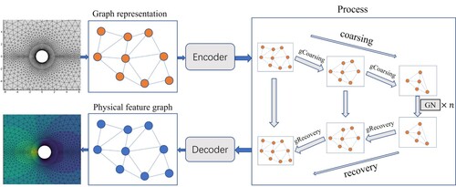
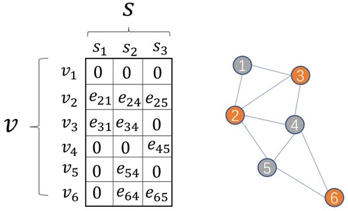
Figure 2. An example of a graph containing six nodes forming the prolongation matrix P. The coarsened node set S contains $(1,4,5)$ and the fine node set V includes $(1,2,3,4,5,6)$.

3.3. Encoder

The input of our model is a graph $G=(V,E)$, $V\in R^{n\times l}$, $E\in R^{r\times m}$. We initialise node features using the same method as de Avila Belbute-Peres et al. (2020) and the edge features are initialised with the distance between two nodes of the edge. Encoder embeds the graph features into a high-dimensional latent vector using Multi-Layer Perceptrons (MLPs). (2) $\begin{array}{rl}& V_i=[po{s}_i,PhysicalParameters],E_{ij}=\left[u\right(po{s}_i,po{s}_j\left)\right]\end{array}$(2) (3) $\begin{array}{rl}& v_i=ML{P}_v\left(V_i\right),e_{ij}=ML{P}_e\left(E_{ij}\right)\end{array}$(3) $po{s}_i$ is the coordinate of the node i and PhysicalParameters are some scalars, such as Mach number and AOA in the airfoil scenario or Reynolds number in the cylinder flow scenario. $u(po{s}_i,po{s}_j)$ represents the distance between node i and node j.

3.4. Algebraic multigrid-based graph coarsing layer

The algebraic multigrid-based graph coarsing layer firstly uses a GN block (Sanchez-Gonzalez et al., 2018) to summarise and extract features of the graph through message passing. In the GN block, nodes aggregate information from all their neighbouring nodes and uses the aggregated information to update features. The message passing of each block is exhibited in Equation (4(4) $e_{ij}=ML{P}_e(e_{ij}^{\mathrm{\prime }},v_i,v_j),v_i=ML{P}_v(v_i^{\mathrm{\prime }},\sum _{j\in N_i}{e}_{ij})$(4) ). $e_{ij}^{\mathrm{\prime }}$ and $v_i^{\mathrm{\prime }}$ are the outputs of the previous block. $N_i$ is the set of neighbouring nodes of i. (4) $e_{ij}=ML{P}_e(e_{ij}^{\mathrm{\prime }},v_i,v_j),v_i=ML{P}_v(v_i^{\mathrm{\prime }},\sum _{j\in N_i}{e}_{ij})$(4) For coarsening of the graph, we firstly use the traditional algebraic multigrid algorithm Ruge–Stuben method (RS) (Ruge & Stüben, 1987) as implemented in Olson and Schroder (2018) to classify all nodes into a coarsened node set S and a fine node set V, where coarsened nodes are a subset of fine nodes. The nodes of the coarse graph are the set of coarsened node S. The most critical step of the algebraic multigrid algorithm is to obtain the prolongation matrix P. The method mentioned from Luz et al. (2020) is adopted to get the prolongation matrix P. Then a GN block is employed to update features of the edges and the updated features are used as the weights of the edges in the prolongation matrix P. (5) $\begin{array}{rl}e& =GN(v^{\mathrm{\prime }},e^{\mathrm{\prime }})\end{array}$(5) (6) $\begin{array}{rl}{P}_{ij}& =\{\begin{array}{ll}{e}_{ij}& \mathrm{i}\mathrm{f}{E}_{ij}\in E_G\\ 0& \mathrm{i}\mathrm{f}{E}_{ij}\notin E_G\end{array}\end{array}$(6) The coarsened node set S corresponds to the columns of the prolongation matrix P, while the fine node set V corresponds to the rows. If an edge of the prolongation matrix P exists in the set of edges of the graph, then $p_{ij}=e_{ij}$, otherwise $p_{ij}=0$. When the fine graph is coarsen, the new adjacency matrix $A^c$ is constructed to maintain the connectivity of the coarser graph (Ranjan et al., 2020; Ying et al., 2018). We use the prolongation matrix P and the adjacency matrix of the graph to obtain the connectivity relations of the coarsened graph. (7) $A^c=P^{T}AP,\mathrm{w}\mathrm{h}\mathrm{e}\mathrm{r}\mathrm{e}P\in R^{n\times c},A\in R^{n\times n},A^c\in R^{c\times c}$(7) A is the adjacency matrix of the fine graph. $A^c$ is the adjacency matrix of the coarsened graph. If $A_{ij}^c$ in $A^c$ is not 0, then there exists an edge $E_{ij}$ in the coarsened graph and the features $e_{ij}$ of the edge is $A_{ij}^c$. The linkage relation of the coarsened graph, the edge set $E^c$ and edge features $e^c$ are obtained. The algebraic multigrid-based graph coarsening algorithm is shown in Algorithm 2.

3.5. Graph recovery layer

In algebraic multigrid-based graph coarsening layers, we coarsen the graph to different scales and then use GN blocks to summarise and extract features of the graph through message passing. The graph recovery layer employs a reverse operation compared with the algebraic multigrid-based graph coarsening layer. In the graph recovery layer, we upsample the graph using spatial interpolation method (Qi et al., 2017). $F\in R^{n\times r}$ is the node features of the graph we want to recover and the node set of the graph is $X_f$. $C\in R^{m\times r}$ is the node features of coarsened graph and the node set of coarsened graph is $X_c$. $r_j=h_j,j\in X_c,h_j$ is features of node j appearing in $X_c$ and $r_j$ is features of node j appearing in $X_f$. Node i, which appears in $X_f$ but not in $X_c$, can locate k closest nodes in $X_c$. Then the features $r_i$ of node i is calculated by the following equation: (8) $r_i=\sum _{j\in k}\frac{w_{ij}{h}_j}{\sum _{j\in k}{w}_{ij}},\mathrm{w}\mathrm{h}\mathrm{e}\mathrm{r}\mathrm{e}{w}_{ij}=\frac{1}{d(X_f^i,X_c^j)}$(8) Here $d(X_f^i,X_c^j)$ is the spatial distance between nodes i and j. Each node $i\in X_f$ has a representation $r_i$ so that we recover C to F. After each upsampling, we then use fully connected layers to extract features similar to the post-smooth step in the algebraic multigrid algorithm. (9) $h_i=MLP\left(r_i\right),h_i\in F$(9)

3.6. The prolongation version of AMGNET

The prolongation version of AMGNET is to explore the effect of using the constructed P-based method and the spatial interpolation method in the graph recovery layer on the prediction accuracy of the model. In the algebraic multigrid algorithm, after reducing the solution matrix using the constructed P, the coarse-level solutions are prolonged using the constructed P, and then the prolonged solutions are added to the fine-level solution. According to Equation (7(7) $A^c=P^{T}AP,\mathrm{w}\mathrm{h}\mathrm{e}\mathrm{r}\mathrm{e}P\in R^{n\times c},A\in R^{n\times n},A^c\in R^{c\times c}$(7) ), we use the constructed P to coarsen the fine graph to the coarser graph. In contrast, the prolongation version of AMGNET uses the constructed P-based method to recover the node features of the graph in the graph recovery Layer. (10) $V_{\mathrm{f}\mathrm{i}\mathrm{n}\mathrm{e}}=P{V}_{\mathrm{c}\mathrm{o}\mathrm{a}\mathrm{r}\mathrm{s}\mathrm{e}\mathrm{n}},\mathrm{w}\mathrm{h}\mathrm{e}\mathrm{r}\mathrm{e}{V}_{\mathrm{c}\mathrm{o}\mathrm{r}\mathrm{s}\mathrm{e}\mathrm{n}}\in R^{n_2\times c},V_{\mathrm{f}\mathrm{i}\mathrm{n}\mathrm{e}}\in R^{n_1\times c},P\in R^{n_1\times n_2}$(10) The constructed P-based method directly use the prolongation matrix P to recover the node features of fine graph from that of the coarse graph. $V_{\mathrm{c}\mathrm{o}\mathrm{a}\mathrm{r}\mathrm{s}\mathrm{e}\mathrm{n}}$ is node features of the coarse graph and $V_{\mathrm{f}\mathrm{i}\mathrm{n}\mathrm{e}}$ is node features of the fine graph.

3.7. Model training

The flow fields $Z\in R^{N\times 3}$ that AMGNET predicts, which contains the pressure as well as the velocity in the x and y directions at all nodes in the fine mesh. We employ the mean squared error (MSE) loss ℓ between the predicted flow field $\hat{Z}$ and the ground truth and minimise this loss ℓ. (11) ${\ell }_{graph}=\Vert Z-\hat{Z}{\Vert }^2$(11) The ground truth Z in airfoil and cylinder is obtained by running the simulation solver for iterative computation until convergence. The Adam optimiser (Kingma & Ba, 2014) is employed to minimise the loss with a learning rate $\alpha =5\cdot {10}^{-4}$ for the airfoil and a learning rate $\alpha =1\cdot {10}^{-4}$ in the cylinder flow.

4. Experiments

Our model is evaluated in two different physical scenarios, as is shown in Figure 3, including the flow over airfoil and cylinder. Airfoil dataset comes from de Avila Belbute-Peres et al. (2020). The airfoil dataset employs the NACA0012 airfoil and the mesh representing the airfoil contains 6648 nodes. The mesh of cylinder contains 3887 nodes. All meshes are composed of triangular and quadrilateral elements. Airfoil cases are governed by the Navier–Stokes equations (Euler equations) under steady-state, compressible, and inviscid conditions. Cylinder cases are governed by the Navier–Stokes equations (Euler equations) under steady-state, incompressible, and inviscid conditions. All cases are run to convergence, and Table 1 shows the details for both datasets.

Figure 3. (a) flow over a cylinder with varying Reynolds number; (b) high-speed flow over a airfoil with different initial Mach Number and AoA.

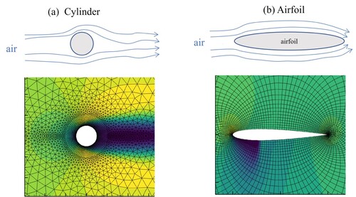
Figure 4. Training curves for the both tasks. The vertical axis represents the root mean squared error (RMSE). AMGNET and AMGNET(prolongation) converges faster than the GCN baseline model in the cylinder task. AMGNET converges faster than the GCN baseline model in the airfoil task.

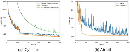
Table 1. Below the details of the datasets are shown. “PDEs” describes the underlying PDE. Airfoil employs compressible Navier-Stokes flow and cylinder employs incompressible Navier-Stokes flow. “Type” describes the type of Navier-Stokes equations.

Dataset	PDEs	Type	Meshing	Node Number
Airfoil	compressible NS	Eulerian	unstructual	6684
Cylinder	incompressible NS	Eulerian	unstructual	3887

In the datasets, the training set is defined by $\begin{array}{rl}& Ao{A}_{\mathrm{t}\mathrm{r}\mathrm{a}\mathrm{i}\mathrm{n}}=\{-10,-9,\dots ,9,10\},\\ & Mac{h}_{\mathrm{t}\mathrm{r}\mathrm{a}\mathrm{i}\mathrm{n}}=\{0.2,0.3,0.35,0.4,0.5,0.55,0.6,0.7\},\\ & Reynoldsnumbe{r}_{\mathrm{t}\mathrm{r}\mathrm{a}\mathrm{i}\mathrm{n}}=\{1.0,1.5,2,\dots ,37.5,38,38.5\}.\end{array}$Similarly, the testing set is defined by $\begin{array}{rl}& Ao{A}_{\mathrm{t}\mathrm{e}\mathrm{s}\mathrm{t}}=\{-10,-9,\dots ,9,10\},\\ & Mac{h}_{\mathrm{t}\mathrm{e}\mathrm{s}\mathrm{t}}=\{0.25,0.45,0.65\},\\ & Reynoldsnumbe{r}_{\mathrm{t}\mathrm{e}\mathrm{s}\mathrm{t}}=\{3.5,10,\dots ,33,39\}.\end{array}$In airfoil scenario, training pairs are then sampled uniformly from $Ao{A}_{\mathrm{t}\mathrm{r}\mathrm{a}\mathrm{i}\mathrm{n}}\times Mac{h}_{\mathrm{t}\mathrm{r}\mathrm{a}\mathrm{i}\mathrm{n}}$, and test pairs from $Ao{A}_{\mathrm{t}\mathrm{e}\mathrm{s}\mathrm{t}}\times Mac{h}_{\mathrm{t}\mathrm{e}\mathrm{s}\mathrm{t}}$ (de Avila Belbute-Peres et al., 2020). In cylinder flow scenario, training datas come from $Reynoldsnumbe{r}_{\mathrm{t}\mathrm{r}\mathrm{a}\mathrm{i}\mathrm{n}}$ and test datas from $Reynoldsnumbe{r}_{\mathrm{t}\mathrm{e}\mathrm{s}\mathrm{t}}$.

For the AMGNET, we use 2 layers of graph coarsening layer and 4 GN blocks, besides 2 layers of graph recovery layer. In GN block, the node and edge functions ($ml{p}_v,ml{p}_e$) are MLPs with two hidden layers of size 128, and ReLU activation. In the graph recovery layer, we use MLPs with four hidden layers of size 128. The batch size for all experiments is set to 4. The k of the spatial interpolation method is set to 3 in the graph recovery layer.

In our experiments, two benchmarks, the GCN and the prolongation versions of AMGNE are compared with our model. The GCN baseline consists of 6 GCN layers with 512 channels (de Avila Belbute-Peres et al., 2020). The prolongation version of AMGNET uses the constructed P-based method in the graph recovery layer instead of the spatial interpolation method.

Computational costs. Table 2 shows the computational efficiency of our model with benchmarks as well as simulation solver for both datasets. Even though our approach is less computationally efficient than the GCN baseline, the simulation solver is still slower than our model by one order of magnitude on bath datasets. The efficiency advantage of our model means that it can be used for more complex physical scenarios that require more computational costs.

Table 2. Runtime. Runtimes for a batch of 4 predictions of our model and GCN baseline as well as AMGNET(prolongation) compared to ground truth simulations, where time units are in seconds.

Model	AMGNET	GCN	AMGNET(prolongation)	Ground truth simulation
Airfoil	16	0.02	10.5	137
Cylinder	10	0.04	10.7	800

Notes: Deep learning models significantly faster than ground truth simulation. Our model runs on a 48-core, 2.0 GHz machine with an NVidia Ampere A100 GPU.

4.1. Comparison with GCN in different physical scenarios

Our model requires as input some physical parameters, which controll the behaviour of the fluid. The physical parameter scalars used in the airfoil are the AOA and Mach number, and the physical parameter scalar is the Reynolds number in the cylinder flow. We use the same inputs as in the GCN baseline, and we initialise the node features using the coordinates of the mesh nodes and the physical parameter scalars. Our learning model predicts the flow fields under the given physical parameters. To quantitatively evaluate our model and the GCN baseline, we calculate the root mean square error (RMSE) of the predictions for whole domain flow field region. Table 3 exhibits the prediction errors of AMGNET and GCN on the two datasets. Our model predicts better than the GCN model. Scales of the mesh range from a few meters to a few millimeters, enabling the flow field to have ultra-high resolution. By presenting the results of flow field prediction on a small-scale mesh, the prediction accuracy of models can be evaluated more effectively. Figure 5 exhibts the prediction of the velocity field in the x direction around the airfoil for both models with AOA = 8.0 and Mach Number equals to 0.65. Figure 6 exhibts the prediction of the velocity field in the x direction over the cylinder for both models with Reynolds number equals to 78. The pressure distribution near the boundary and the contour figures can be found in Appendix (Figures A1 and A2). The flow field prediction errors of our model are significantly less than that of the GCN model from the experimental results of the both tasks.

GCN aggregates information from neighbouring nodes and computes messages on nodes. In the GCN baseline model, the connectivity of the graph is kept constant and the message passing of nodes takes place at the fixed neighbouring nodes in each GCN layer. The over-smooth of message passing of GCN and the lack of message passing information make the GCN more prone to overfitting and thus do not learn the local general rules well (Pfaff et al., 2021). GN is able to extract more complex graph features due to computing message on edges and nodes. In AMGNET, the graph is coarsened using the coarsening layer and the nodes of the coarser graph aggregate the features of the neighbouring nodes that have been coarsened. When computing messages in the next layer, each node passes more features, because each node also contains the features of those nodes that are coarsened. In AMGNET, the connection relation of the graph in each layer is changed by coarsening, and the neighbouring nodes of nodes are not fixed. The message passing of node features has larger receptive fields. Therefore, our model has better generalisation capability and can effectively improve the accuracy of flow field prediction.

Figure 5. AMGNET model prediction, ground truth and GCN model prediction for airfoil with AOA $=8.0$ and Mach Number $=0.65$. The x direction velocity field is presented here.

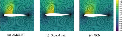
Figure 6. AMGNET model prediction, ground truth and GCN model prediction for the cylinder flow with Reynolds number = 78. The y direction velocity field is presented here.

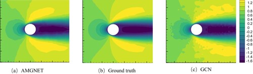
Table 3. RMSE on the testing set for the airfoil and cylinderflow tasks.

Model	Airfoil	Cylinder
GCN	$2.0\cdot {10}^{-2}$	$5.2\cdot {10}^{-2}$
AMGNET	$1.4\cdot {10}^{-2}$	$2.7\cdot {10}^{-2}$

Notes: The AMGNET is compared to GCN baseline. In the cylinder task, the two models run for 500 epochs. The GCN baseline run for 500 epochs and AMGNET run for 120 epochs in airfoil task. The prediction error of our model is less than that of the GCN baseline in both physical cases in both physical scenarios.

4.2. Comparison with the prolongation version of AMGNET in different physical scenarios

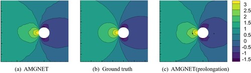
With the purpose of exploring the impact of different mesh recovery methods on the prediction results, we compare AMGNET with the prolongation version of AMGNET. Table 4 shows the average prediction errors of AMGNET and the prolongation version of AMGNET on the two datasets. Figure 7 exhibits the predicted results of pressure field of the airfoil for both models with AOA = 8.0 and Mach Number equals to 0.65. Near the upper boundary of the airfoil, the prediction error of AMGNET is smaller than that of AMG (prolongation) when compared with Ground truth. Figure 8 exhibits the pressure field of the cylinder flow for both models with Reynolds number equals to 78. The predicted results of AMGNET (prolongation) appear noisy, while AMGNET does not. The prediction results of AMGNET are better than AMGNET (prolongation). The results show that the graph recovery using the spatial interpolation method has smaller prediction errors.

Figure 7. AMGNET model prediction, ground truth and AMGNET(prolongation) model prediction for airfoil with AOA = 8.0 and Mach Number = 0.65. Shown in the above figure is the pressure field.

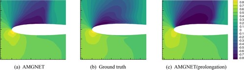
Figure 8. AMGNET model prediction, ground truth and AMGNET(prolongation) model prediction for the cylinder flow with Reynolds number = 78. Shown in the above figure is the pressure field.

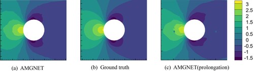
Table 4. RMSE on the testing set for the airfoil and cylinderflow tasks.

Model	Airfoil	Cylinder
AMGNET(prolongation)	$2.0\cdot {10}^{-1}$	$4.6\cdot {10}^{-2}$
AMGNET	$1.4\cdot {10}^{-2}$	$2.7\cdot {10}^{-2}$

Note: The AMGNET is compared to AMGNET(prolongation). In the cylinder task, the two models run for 500 epochs and the two models run for 120 epochs in airfoil task.

The results as described above are due to the following. Node features of the graph are recovered directly using the prolongation matrix P multiplied with the node feature matrix in the constructied P-based recovery method. This method causes the features to fluctuate and is difficult to converge in the MLPs of the graph recovery layer. In the spatial interpolation method, features of the nodes originally belonging to the coarsen graph come directly from the coarse graph and the features of the nodes that need to be recovered are recovered using interpolation to make the feature smooth. It is easier to converge in the MLPs of the graph recovery layer.

In addition, the effectiveness of our method is evaluated by exploring the prediction results for different numbers of graph neural network layers. GN-only contains only the GN block and does not contain any graph coarsening and graph recovery layers. AMGNET(1-1) employs one graph coarsing Layer and one graph recovery layer as well as 7 GN blocks. Table 5 shows the average prediction errors of AMGNET and other models on the two datasets. From the experimental results, comparing GCN models with GN-only models, our model has smaller prediction errors. The experimental results demonstrate that our multi-scale graph learning method enables GNNs to learn local general rules to improve the accuracy of flow field prediction and reduce the prediction error of physical problems. The multi-scale graph representation allows nodes to have higher-order features, since the nodes of the graph contain those node features that are coarsened. The message passing of graph neural networks is able to deliver more messages, increasing the perceptual field of the nodes, which is consistent with the idea of the pooling. It makes the message passing more efficient. As shown in the training curves Figure 4, our model has faster convergence.

Table 5. RMSE on the testing set for the airfoil and cylinderflow tasks.

Model	Airfoil	Cylinder
GN-only(9 layers)	$2.1\cdot {10}^{-2}$	$3.1\cdot {10}^{-2}$
GCN(9 layers)	$1.6\cdot {10}^{-2}$	$5.3\cdot {10}^{-2}$
AMGNET(1-1)	$2.8\cdot {10}^{-2}$	$4.4\cdot {10}^{-2}$
AMGNET	$1.4\cdot {10}^{-2}$	$2.7\cdot {10}^{-2}$

Notes: The AMGNET is compared to other models with different numbers of network layers. All models run for 500 epochs in both tasks.

5. Computational complexity

The implementation of our model consists of the encoder, the decoder, the algebraic multigrid-based graph coarsing layers and the graph recovery layers. $|V|$ represents the number of vertices of the graph and $|E|$ represents the number of edges of the graph. The time complexity of the encoder and decoder is $O(L\times (|V|+|E|)\times F\times F^{\mathrm{\prime }})$, where F represents the original feature dimension and $F^{\mathrm{\prime }}$ represents the latent feature dimension, while L is the number of layers of MLPs.

The algebraic multigrid-based graph coarsing layer contains two GN layers and the graph coarsening operation as well as the graph connectivity maintenance operation. The time complexity of the GNs is $O\left(\right(|V^{\mathrm{\prime }}|+|E^{\mathrm{\prime }}|)\times F^{\mathrm{\prime }}\times F^{\mathrm{\prime }})$, where $N^{\mathrm{\prime }}$ is the number of nodes and $E^{\mathrm{\prime }}$ is the number of edges in this layer. The graph coarsening operation RS method takes time $O\left(|V{|}^2\right)$ and the new graph connectivity generated by galerkin product takes time $O(F^{\mathrm{\prime }}\times |V{|}^3)$. In the graph recovery layer, the MLPs have conputation time $O(N^{\mathrm{\prime }}\times F^{\mathrm{\prime }}\times F^{\mathrm{\prime }})$ and the time complexity of spatial interpolation method is $O\left(N^{\mathrm{\prime }}\right)$. The spatial overhead of our model is linearly related to the number of nodes and edges of the mesh. The memory usage of our model is 6G in the airfoil dataset and is 4G in the cylinder dataset. From the above analysis, it can be seen that the sparse matrix multiplication in the operation of maintaining graph connectivity relations is the most time-consuming part of the computational overhead.

6. Conclusion

In this paper, we propose a multi-scale graph neural networks model, called AMGNET, which learns graph features from different mesh scales by using the algebraic multigrid-based approach. Based on the idea of pooling, the coarsening method of algebraic multigrid is used to coarsen the mesh graph. The coarsening enables to obtain graph representations of different scales. Multi-scale graph representations learning can improve the learning ability of the model for graph features, thus upgrading the prediction accuracy of the flow field. For our experiments, it is demonstrated that the multi-scale graph learning model enhances feature learning capability and effectively improves the accuracy of flow field prediction.

Although it is shown from experiments that our model improves the accuracy of flow field prediction, it introduces some performance overhead because our model needs to acquire multi-scale graph representations. It is necessary to use sparse matrix multiplication in order to maintain the connectivity of the graphs at different scales, which causes some computational costs of our model. As can be seen from Table 2, the computational efficiency of our AMGNET is lower than that of the GCN model. Also the multiplication of sparse matrices greatly increases the training time of our model. The training time is about 5 hours to reach the loss convergence in the cylinder task, while it takes 10 hours in the airfoil task. In the future, our work will optimise the graph coarsening method to reduce the computational complexity of our model in predicting flow fields and apply multi-scale graph learning models to the dynamical state prediction of physical systems.

Disclosure statement

No potential conflict of interest was reported by the author(s).

Additional information

Funding

This work is supported by National Key Project of China [grant number GJXM92579].

Appendix. The pressure coefficients figures and the contour figures

Figures A1 and A2 show the pressure coefficients on the boundary of the airfoil and the cylinder. To better show the comparison between the predicted flow field of our AMGNET model and the GCN baseline model and the ground truth, contour figures are presented below (Figures A3 –A6).

Figure A1. AMGNET model, ground truth and GCN model for airfoil with AOA = 8.0 and Mach Number = 0.65. The pressure coefficients of x-axis direction is presented here.

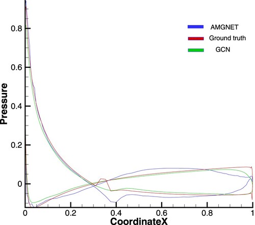
Figure A2. AMGNET model, ground truth and GCN model for cylinder with Reynolds number = 78. The pressure coefficients of x-axis direction is presented here.

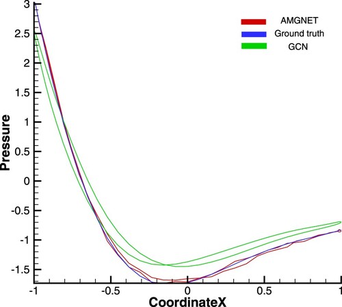
Figure A3. AMGNET model prediction, ground truth and GCN model prediction for airfoil with AOA = 8.0 and Mach Number = 0.65. The above figure shows the velocity field in the x direction.

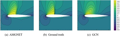
Figure A4. AMGNET model prediction, ground truth and GCN model prediction for the cylinder flow with Reynolds number = 78. The above figure shows the velocity field in the y direction.

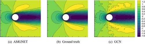
Figure A5. AMGNET model prediction, ground truth and AMGNET(prolongation) model prediction for airfoil with AOA = 8.0 and Mach Number = 0.65. Shown in the above figure is the pressure field.

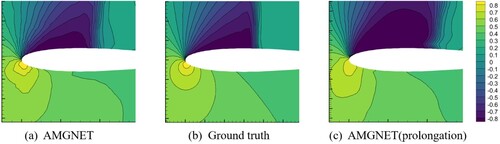
Figure A6. AMGNET model prediction, ground truth and AMGNET(prolongation) model prediction for the cylinder flow with Reynolds number = 78. Shown in the above figure is the pressure field.

References

- Afshar, Y., Bhatnagar, S., Pan, S., Duraisamy, K., & Kaushik, S. (2019, August). Prediction of aerodynamic flow fields using convolutional neural networks. Computational Mechanics, 64(2), 525–545. https://doi.org/10.1007/s00466-019-01740-0
- Battaglia, P. W., Hamrick, J. B., Bapst, V., Sanchez-Gonzalez, A., Zambaldi, V., Malinowski, M., & Faulkner, R. (2018). Relational inductive biases, deep learning, and graph networks. arXiv preprint arXiv:1806.01261
- Braess, D., & Hackbusch, W. (1983). A new convergence proof for the multigrid method including the v−cycle. SIAM Journal on Numerical Analysis, 20(5), 967–975. https://doi.org/10.1137/0720066
- Brandt, A., McCormick, S. F., & Ruge, J. (1984). Algebraic multigrid (AMG) for sparse matrix equations. In D. J. Evans (Ed.), Sparsity and its applications (pp. 257–284). Cambridge University Press.
- Chang, F., Ge, L., Li, S., Wu, K., & Wang, Y. (2021). Self-adaptive spatial-temporal network based on heterogeneous data for air quality prediction. Connection Science, 33(3), 427–446. https://doi.org/10.1080/09540091.2020.1841095
- de Avila Belbute-Peres, F., Economon, T. D., & Kolter, J. Z. (2020). Combining differentiable PDE solvers and graph neural networks for fluid flow prediction. In Proceedings of the 37th international conference on machine learning (icml 2020) (pp. 2402–2411). PMLR.
- Gao, H., & Ji, S. (2019). Graph u-nets. In International conference on machine learning (pp. 2083–2092). PMLR.
- Gilmer, J., Schoenholz, S. S., Riley, P. F., Vinyals, O., & Dahl, G. E. (2017). Neural message passing for quantum chemistry. In Proceedings of the 34th international conference on machine learning(Vol. 70, pp. 1263–1272). JMLR.
- Gori, M., Monfardini, G., & Scarselli, F. (2005). A new model for learning in graph domains. In Proceedings of the 2005 IEEE international joint conference on neural networks, 2005 (Vol. 2, pp. 729–734). IEEE.
- Guo, X., Li, W., & Iorio, F. (2016). Convolutional neural networks for steady flow approximation. In Proceedings of the 22nd ACM SIGKDD international conference on knowledge discovery and data mining (pp. 481–490). ACM.
- Han, X. (2022). Predicting physics in mesh-reduced space with temporal attention. In International conference on learning representations. OpenReview.net.
- Hartmann, D., Lessig, C., Margenberg, N., & Richter, T. (2020). A neural network multigrid solver for the navier-stokes equations. arXiv preprint arXiv:2008.11520
- Hu, N., Zhang, D., Xie, K., Liang, W., & M. Y. Hsieh (2022). Graph learning-based spatial-temporal graph convolutional neural networks for traffic forecasting. Connection Science, 34(1), 429–448. https://doi.org/10.1080/09540091.2021.2006607
- Kingma, D. P., & Ba, J. (2014). Adam: a method for stochastic optimization. arXiv preprint arXiv:1412.6980
- Kipf, T. N., & Welling, M. (2016). Semi-supervised classification with graph convolutional networks. arXiv preprint arXiv:1609.02907
- Luz, I., Galun, M., Maron, H., Basri, R., & Yavneh, I. (2020). Learning algebraic multigrid using graph neural networks. In Proceedings of the 37th international conference on machine learning (p. 119). PMLR.
- Olson, L. N., & Schroder, J. B. (2018). PyAMG: algebraic multigrid solvers in Python v4.0. URL https://github.com/pyamg/pyamg. Release 4.0.
- Pfaff, T., Fortunato, M., Sanchez-Gonzalez, A., & Battaglia, P. W. (2021). Learning mesh-based simulation with graph networks. In International conference on learning representations. OpenReview.net.
- Qi, C. R., Yi, L., Su, H., & Guibas, L. J. (2017). Pointnet++: deep hierarchical feature learning on point sets in a metric space. In Advances in neural information processing systems (pp. 5099–5108). MIT Press.
- Ranjan, E., Sanyal, S., & Talukdar, P. (2020, April). Asap: adaptive structure aware pooling for learning hierarchical graph representations. In Proceedings of the AAAI Conference on Artificial Intelligence (Vol. 34, No. 4, pp. 5470–5477). AAAI.
- Ruge, J. (1983). Algebraic multigrid (AMG) for geodetic survey problems. In Proceedings of the international multigrid conference.
- Ruge, J., & Stüben, K. (1987). Algebraic multigrid (AMG). In S. F. McCormick (Ed.), Multigrid methods, frontiers in applied mathematics (pp. 73–130). SIAM.
- Sanchez-Gonzalez, A., Godwin, J., Pfaff, T., Ying, R., Leskovec, J., & Battaglia, P. (2020). Learning to simulate complex physics with graph networks. In International conference on machine learning (pp. 8459-8468). PMLR.
- Sanchez-Gonzalez, A., Heess, N., Springenberg, J. T., Merel, J., Riedmiller, M., Hadsell, R., & Battaglia, P. (2018). Graph networks as learnable physics engines for inference and control. In International conference on machine learning (pp. 4470–4479). PMLR.
- Scarselli, F., Gori, M., Tsoi, A. C., Hagenbuchner, M., & Monfardini, G. (2009). The graph neural network model. IEEE Transactions on Neural Networks, 20(1), 61–80. https://doi.org/10.1109/TNN.2008.2005605
- Seo, S., & Liu, Y. (2019). Differentiable physics-informed graph networks. arXiv preprint arXiv:1902.02950
- Seo, S., Meng, C., & Liu, Y. (2021). Physics-aware difference graph networks for sparsely-observed dynamics. In International conference on learning representations. OpenReview.net.
- Stüben, K. (2001). Algebraic multigrid (AMG): an introduction with applications. In U. Trottenberg, C. Oosterlee, and A. Schüller (Eds.), Multigrid. Academic Press.
- Taghibakhshi, A., MacLachlan, S., Olson, L., & West, M. (2021). Optimization-based algebraic multigrid coarsening using reinforcement learning. In Advances in neural information processing systems. MIT Press.
- Um, K., Hu, X., & Thuerey, N. (2018). Liquid splash modeling with neural networks. Computer Graphics Forum, 37(8), 171–182. https://doi.org/10.1111/cgf.2018.37.issue-8
- Wiewel, S., Becher, M., & Thuerey, N. (2019). Latent space physics: towards learning the temporal evolution of fluid flow. Computer Graphics Forum, 38(2), 71–82. https://doi.org/10.1111/cgf.2019.38.issue-2
- Xu, J., & Duraisamy, K. (2020). Multi-level convolutional autoencoder networks for parametric prediction of spatio-temporal dynamics. Computer Methods in Applied Mechanics and Engineering, 372(4), 113379. https://doi.org/10.1016/j.cma.2020.113379
- Xu, J., Pradhan, A., & Duraisamy, K. (2021). Conditionally parameterized, discretization-aware neural networks for mesh-based modeling of physical systems. arXiv preprint arXiv:2109.09510
- Ying, R., You, J., Morris, C., Ren, X., Hamilton, W. L., & Leskovec, J. (2018). Hierarchical graph representation learning with differentiable pooling. arXiv preprint arXiv:1806.08804
- Ying, Z., You, J., Morris, C., Ren, X., Hamilton, W., & Leskovec, J. (2018). Hierarchical graph representation learning with differentiable pooling. In Proceedings of the 32th international conference on neural information processing systems. MIT Press.
- Yu, F., & Koltun, V. (2016). Multi-scale context aggregation by dilated convolutions. In Proceedings of the international conference on learning representations. OpenReview.net.
- Zhao, C., Li, X., Shao, Z., Yang, H., & Wang, F. (2022). Multi-featured spatial-temporal and dynamic multi-graph convolutional network for metro passenger flow prediction. Connection Science, 34(1), 1252–1272. https://doi.org/10.1080/09540091.2022.2061915