NNNPE: non-neighbourhood and neighbourhood preserving embedding

ABSTRACT

Manifold learning is an important class of methods for nonlinear dimensionality reduction. Among them, the LLE optimisation goal is to maintain the relationship between local neighbourhoods in the original embedding manifold to reduce dimensionality, and NPE is a linear approximation to LLE. However, these two algorithms only consider maintaining the neighbour relationship of samples in low-dimensional space and ignore the global features between non-neighbour samples, such as the face shooting angle. Therefore, in order to simultaneously consider the nearest neighbour structure and global features of samples in nonlinear dimensionality reduction, it can be linearly calculated. This work provides a novel linear dimensionality reduction approach named non-neighbour and neighbour preserving embedding (NNNPE). First, we rewrite the objective function of the algorithm LLE based on the principle of our novel algorithm. Second, we introduce the linear mapping to the objective function. Finally, the mapping matrix is calculated by the method of the fast learning Mahalanobis metric. The experimental results show that the method proposed in this paper is effective.

KEYWORDS:

• Machine learning
• manifold learning
• dimensionality reduction
• neighborhood preserving embedding

1. Introduction

Data dimensionality reduction is an important basic task of pattern recognition, and it is divided into traditional machine learning dimensionality reduction and deep learning-based dimensionality reduction methods. At present, the most commonly used and effective data dimensionality reduction method is automatic feature extraction based on deep learning. For example, high-dimensional raw image data are directly input into the convolutional neural network (CNN), such as ResNet (He et al., 2016), and then a large amount of labelled data are used to drive supervised learning. Subsequently, output effective features are obtained after dimensionality reduction, and the fully connected network is entered for classification. Alternatively, the image is input into the auto-encoder (Baldi, 2012), and unsupervised learning is performed to compress the feature dimension with as little loss of information as possible. The advantage of this type of method is that it does not need to manually design features and can automatically extract features according to the data-driven target. However, the method is also limited by the large amount of training data and lack of interpretability. For fields that focus on interpretability, such as medical data analysis, traditional data dimensionality reduction methods with sound theoretical support are still valuable.

Traditionally, dimensionality reduction is a type of projection method that performs linear projection on incoming data and reduces its dimension from high to low, such as principal component analysis (PCA) (Turk & Pentland, 1991) and linear discriminant analysis (LDA) (Belhumeur et al., 1997). LDA enhances the ratio of between-class to within-class variance to identify an explicit projection, whereas PCA maximises the variance of data in low dimension to train a linear projection. The projection method uses projections to reduce data dimensionality. New linear dimensionality reduction methods have performed well in recent years. Among them, SWRLDA (Yan et al., 2020) can automatically avoid the optimal mean calculation and learn the adaptive weights of class pairs to achieve fast convergence. Chang et al. (2015) proposed a composite rank-k projection algorithm to directly process matrices without converting them to vectors for bilinear analysis. However, these linear dimensionality reduction methods are usually inadequate for dealing with complex nonlinear data.

Another type of traditional data dimensionality reduction method is nonlinear dimensionality reduction. Nonlinear dimensionality reduction methods include methods based on kernel functions (Sumithra & Surendran, 2015; Zhu et al., 2012), early neural networks (Pehlevan & Chklovskii, 2015; Wang et al., 2012), and manifold learning (Cai et al., 2007; Yang et al., 2016). An important problem in various kernel function dimensionality reduction methods is knowing how to choose the kernel function, and the objective function used for dimensionality reduction does not consider maintaining the integrity of its data structure. The methods based on early neural networks, such as multilayer fully connected networks, BP network (Schmidhuber, 2015), etc., have high training complexity and lack interpretability. The goal of manifold learning is to recover the low-dimensional manifold structure from high-dimensional sampling data and obtain the corresponding embedding map to realise data dimensionality reduction or data visualisation, which has good interpretability. Brahma et al. (2015) explained from the perspective of manifold structure that deep learning requires a learning of the hidden manifold structure from high-dimensional data.

Local linear embedding (LLE) and neighbourhood preserving embedding (NPE) (He et al., 2005) strive to preserve each neighbourhood’s local configuration in low-dimensional space as it is in high-dimensional space. Thus, these methods simply preserve each data point’s local relationship during the dimensionality reduction process. However, they ignore the relationship of data points that are far from each other, especially the supervised ones. Dimensionality reduction mainly preserves the intrinsic dimensionality, which is characterised by discrimination. For example, LDA ensures that inter – and intra-class distances are maximised and minimized, respectively. It seeks to preserve the local neighbourhood structure (inside the class) while also maintaining the global non-neighbourhood structure (between-class). Meanwhile, Mahalanobis metric learning (MML) (Zheng et al., 2012) aims to maximise the distance between dissimilar points while decreasing the distance between similar points.

1.1. Main contributions

In this study, motivated by LDA, MML, and NPE, we present a novel linear projection approach, which is a version of supervised NPE. First, we create an adjacency graph per category and compute the weights on the graph’s edges for LLE and NPE. Then, we construct a dissimilar pairwise sample set and a pseudo similar pairwise sample set. By using techniques from MML and ensuring that the mapping function is linear, we can obtain the objective function of this study’s algorithm, particularly the non-neighbourhood and neighbourhood preserving embedding (NNNPE). Finally, binary search and eigenvalue optimisation is employed to efficiently solve the optimisation issue (Bellet et al., 2013). The main contributions and innovations of this work are as follows:

1. Similar to the NPE, the method in this study can provide an ideal linear approximation to the true LLE’s embedding of the underlying data manifold. It does not have to be defined only by the training data points.

2. The difference between this study’s algorithm and NPE is that this work considers the relationship of non-neighbour points, whereas NPE ignores them. Thus, our algorithm can provide a more meaningful representation of the data than NPE.

3. We establish the connection between manifold learning and MML. By using techniques from MML and ensuring that the mapping function is linear, we can obtain an objective function that is similar to that presented in a previous study (Xiang et al., 2008).

4. This method belongs to the traditional nonlinear dimensionality reduction method. It comprehensively considers maintaining local neighbourhood features and global features with good interpretability. It has certain application value in many application fields with strict interpretability requirements, such as the medical field.

The paper is organised as follows. The associated dimension reduction approaches are briefly introduced in Section 2. Section 3 introduces other algorithms and our algorithm, and Section 4 discusses the theoretical justification. Section 5 offers a time-saving approach for resolving the goal function from Section 3. Section 6 presents the experimental outcomes. Section 7 summarises this study.

2. Related works

2.1. Manifold learning

Nonlinear dimensionality reduction approaches, in contrast to linear dimensionality reduction techniques, deal with complex nonlinear data, thus attracting widespread attention. Many nonlinear dimensionality reduction algorithms have been proposed in recent decades, such as isomaps (Tenenbaum et al., 2000), LLE (Roweis & Saul, 2000), Laplacian eigenmaps (LE) (Belkin & Niyogi, 2001), Hessian LLE (Donoho & Grimes, 2003), and LTSA (Zhang & Zha, 2004). These algorithms utilise nonlinear low-dimensional manifolds from sample datasets that are inherent in high-dimensional space. Isomap is a global approach in low-dimensional space that seeks to retain pairwise geodesic distances among data points. By contrast, other techniques are local methods. LLE and LE endeavour to keep the local geometry of data, and neighbour points on the high-dimensional are regarded as neighbouring on the low-dimensional manifold. Hessian LLE is similar to LE in that it replaces the manifold Laplacian with the manifold Hessian. Meanwhile, LTSA is a technique that uses the local tangent space of each sample to characterise the local features of high-dimensional data (Van Der Maaten et al., 2009). These nonlinear dimensionality reduction methods have the advantage of finding manifold embedding owing to the highly nonlinear manifold of real-world data. However, they cannot be defined everywhere.

Most manifold learning techniques, in contrast to linear dimension reduction approaches, do not provide explicit projections for data points. Recently, advancements in effective and efficient algorithms have been achieved for the linearisation of nonlinear manifold learning (LML) techniques. IsoProjection (Cai et al., 2007) is the process of linearising an isomap by first constructing a weighted data graph. The weights are approximate to the geodesic distances on the data manifold, and then the pairwise distances are preserved to determine the linear subspace. OIP is a variation of IsoProjection and considers an explicit orthogonal linear projection. LPP (He & Niyogi, 2003) and NPE (He et al., 2005) are linear approximations of LE and LLE that attempt to keep the local geometry of data. In addition, Yang et al. (2016) proposed a supervised Isomap method called the multimanifold discriminant isomap. On this basis, Zhang et al. (2018) proposed a semi-supervised local multimanifold isomap learning framework.

2.2. NPE

He et al. (2005) extended the LLE algorithm to learn linear projection with eigenvalue optimisation. Suppose that $X=(x_1,\dots x_m)$ is a sample set. The first step is to use K nearest neighbours or $\epsilon$-neighbourhood to create an adjacency graph.

The weights are calculated in the second phase. The weight of the edge is calculated by minimising the objective function as follows: (1) $\begin{array}{r}\begin{array}{l}min\sum _i||x_i-\sum _j{W}_{ij}{x}_j|{|}^2,\\ st.\sum _j{W}_{ij}=1,j=1,2,\dots m\end{array}\end{array}$(1) where $W$ represents the weight matrix, and $W_{ij}$ represents the edge weight from node $i$ to node $j$.

The third step is to compute the projections by minimising the objective function as follows: (2) $\begin{array}{r}{A}^{\ast }=\underset{a^{T}X{X}^{T}a=1}{\text{argmin}}{a}^{T}XMXa.\end{array}$(2)

The transformation vector $a$ is computed according to the minimum eigenvalue solution from the following generalised eigenvector problem: (3) $\begin{array}{r}\begin{array}{c}XM{X}^{T}a=\lambda X{X}^{T}a\end{array}\end{array}$(3) where $\begin{array}{l}\begin{array}{c}X=(x_1,\dots x_m),\end{array}\\ \begin{array}{c}M={(I-W)}^T(I-W),\end{array}\\ \begin{array}{c}I=diag(1,\dots 1).\end{array}\end{array}$

Thus, $AϵR^{n\times d}$ can be composed of $a$, such as $A=(a_1,a_2\dots a_d)$.

3. Method

This section introduces NNNPE, the new linear dimensionality reduction approach proposed in this study. NNNPE is an improved NPE algorithm that retains all the properties of NPE. Therefore, NNNPE is also a linear approximation to the nonlinear dimensionality reduction algorithm LLE. According to a previous study (He et al., 2005), NPE is particularly useful when data points $x_1,\dots x_mϵM$ and $M$ are nonlinear manifolds embedded in $R^n$. We study the supervised situation and suppose that the data points belong to $c$ classes. Let $C=(l_1,\dots l_m)$ denote the data’s category in which $l_i=(1,\dots c)$. The following steps describes the formal algorithmic procedure:

1. Building an adjacency graph: Define $G$ as a graph with $m$ nodes corresponding to data points in the proper order. Add an edge between $x_i$ and $x_j$ of the same category $(l_i=l_j)$.

2. Computing the weights: Each data point is rebuilt using other data points from the same category as the linear coefficients in this stage. Let $W$ be the weight matrix. Thus, the weights $W_{ij}$ can be used to summarise the contribution of the $j$th data points to the $i$th reconstruction. Then, enforce $W_{ij}=0$ if $l_i\ne l_j$ (without an edge between nodes $i$ and $j$). Compute other weights that can best linearly reconstruct $x_i$ from its neighbours, thereby solving the following cost objective function: (4) $\begin{array}{r}\begin{array}{c}min\sum _i||x_i-\sum _j{W}_{ij}{x}_j|{|}^2,\\ st.\sum _j{W}_{ij}=1,j=1,2,\dots m\end{array}\end{array}$(4)

3. Computing the covariance matrix: Compute the covariance matrix of the following pseudo congeneric and heterogeneous point pairs: $\begin{array}{rl}{S}_b& =\underset{}{\sum _{W_{ij}=0}(x_i-x_j){(x_i-x_j)}^T},\mathrm{\#}(5)\end{array}$ $\begin{array}{rl}{S}_w& =\underset{}{\sum _i(x_i-x_j^i){(x_i-x_j^i)}^T},\mathrm{\#}(6)\end{array}$where $x_j^i$ is the linear reconstruction of $x_i$, and $x_j^i=\sum _j{W}_{ij}{x}_j$.

4. Computing the projections: Compute the linear mapping matrix $A\in R^{n\times d}$, and then compute the embedding, i.e. $y_i=A^T{x}_i$. The following objective function can be used to obtain the best projections: (7) $\begin{array}{r}\begin{array}{c}{A}^{\ast }=\underset{A^{T}A=I}{\text{argmax}}\left(\frac{tr(A^T{S}_{b}A)}{tr(A^T{S}_{w}A)}\right).\end{array}\end{array}$(7)

The formulation can be regarded as an MML problem and can be efficiently solved, as shown in Section 5.

The above algorithm procedure is supervised. The first step is to construct the adjacency graph with category information, with the resulting graph being an undirected graph. However, this algorithm is also suitable for unsupervised situations. We can use the K-NN algorithm to build the adjacency graph and then add a directed edge from node $i$ to node $j$ if $x_j$ is among the K nearest neighbours of $x_i$. This graph is a directed graph. The rest of the steps are the same.

4. Theoretical justification

The theoretical derivation of our algorithm, which is essentially based on LLE and NPE, is presented in this section.

4.1 Optimal linear embedding

LLE is a local dimensionality reduction approach, and it attempts to maintain only the local attributes of the data. The local attributes of the data manifold are produced in LLE by writing the data points as a linear combination of their nearest neighbours. Although many real-world data have nonlinear manifold distributions, we can assume that the manifold is locally linear. Linear coefficients $W\in R^{m\times m}$ (reconstruction weights) that reconstruct each data point from its neighbours can characterise the local geometry of these patches. The following cost formula is used to calculate the reconstruction errors: (8) $\begin{array}{r}\epsilon (W)=\sum _i||x_i-\sum _j{W}_{ij}{x}_j|{|}^2,\end{array}$(8)

To compute the weights, we subject the minimisation of the cost function to two constraints: $W_{ij}=0$ if $x_j$ is not the neighbourhood of $x_i$, and the rows of the weight matrix sum to one is $\sum _j{W}_{ij}=1$.

In the lower-dimensional space, the reconstruction weights are preserved by the LLE algorithm. In other words, in low-dimensional data representation, the weight matrix may reconstruct data point $y_i$ from its neighbours. Let the sub-manifold $Y$ denote the following d-dimensional data representation $Y=(y_1,\dots ,y_m)\in R^{d\times m}$. This scheme can be obtained by minimising the cost function as follows: (9) $\begin{array}{r}\mathrm{\Phi }(Y)=\sum _i||y_i-\sum _j{W}_{ij}{y}_j|{|}^2.\end{array}$(9)

In this case, the NPE algorithm transforms the cost function by introducing a linear transformation matrix $A\in R^{n\times d}$ as follows: (10) $\begin{array}{r}\mathrm{\Phi }(A)=\sum _i||A{x}_i-\sum _j{W}_{ij}A{x}_j|{|}^2.\end{array}$(10)

The low-dimensional embedding can be obtained by $Y=A^{T}X$. Here, we describe a new cost function. The LLE and NPE both preserve the local manifold structure but ignore its global counterpart. Each data point can be represented as a linear combination of its neighbours; furthermore, through the relationships between non-neighbouring data points, the data point can also be represented by the “local structure” and “global structure.” The essence of dimensionality reduction is to preserve the intrinsic characteristics of data. The intrinsic dimensionality of data refers to the smallest number of parameters required to account for their observed qualities. Each intrinsic dimensionality has a powerful ability to establish the distinctions, even in low-dimensional space. After dimensionality reduction, these data points in the same or different regions take either the same form or different types. LDA may maximise the ratio of between-class to within-class variance. Then, we introduce the global property ignored by the LLE algorithm. We expect the non-neighbouring data points to be separated as far as possible in the low-dimensional space while preserving the neighbourhood relationships. Thus, we propose a new cost function as follows: (11) $\begin{array}{r}min\mathrm{\Phi }(Y)=\frac{{\sum }_i||y_i-{\sum }_j{W}_{ij}{y}_j|{|}^2}{{\sum }_{W_{ij}=0}||y_i-y_j|{|}^2}.\end{array}$(11)

We introduce the linear matrix $A=(a_1,a_2,\dots ,a_d)$ to linearise the cost function similar to that in the NPE algorithm. (12) $\begin{array}{rl}min\underset{}{\mathrm{\Phi }(A)}& =\frac{{\sum }_i||A^T{x}_i-A^T{\sum }_j{W}_{ij}{x}_j|{|}^2}{{\sum }_{W_{ij}=0}||A^T{x}_i-A^T{x}_j|{|}^2},\\ & =\frac{{\sum }_i{(A^T{x}_i-A^T{x}_j^i)}^T(A^T{x}_i-A^T{x}_j^i)}{{\sum }_{W_{ij}=0}{(A^T{x}_i-A^T{x}_j)}^T(A^T{x}_i-A^T{x}_j)},\\ & =\frac{tr(A^T{S}_{w}A)}{tr(A^T{S}_{b}A)},\end{array}$(12) where $x_j^i=\sum _j{W}_{ij}{x}_j$ denotes the reconstructed data point of $x_i$ from its neighbours. We define two sets of pairwise constraints, including pseudo congeneric point pairs [$S=\{x_i,x_j^i{\}}_{i=1}^m$] and heterogeneous point pairs [$D=\{x_i,x_j|W_{ij}=0\}$]. Here, $S_w$ and $S_b$ are the respective covariance matrices of the point pairs in $S$ and $D$. (13) $\begin{array}{rl}{S}_w& =\sum _{(x_i,x_j^i)\in S}(x_i-x_j^i)(x_i-x_j^i{)}^T\end{array}$(13) (14) $\begin{array}{rl}{S}_b& =\sum _{(x_i,x_j)\in D}(x_i-x_j)(x_i-x_j{)}^T\end{array}$(14)

To avoid degenerate solutions, we use the LLE algorithm to constrain the solution vectors $y_i^r$ ($i$th row vector of $Y$) as $y{}_i^{rT}\times y_i^r=1$. We also impose the constraint on matrix $A$ to satisfy $A^{T}A=I$. Finally, we obtain the optimal projections by solving the following objective function: (15) $\begin{array}{r}{A}^{\ast }=\underset{A^{T}A=I}{\text{argmin}}\frac{tr(A^T{S}_{w}A)}{tr(A^T{S}_{b}A)}.\end{array}$(15)

The problem is similar to the MML problem. In the next section, we will introduce the connection between linear manifold learning and MML.

4.2. Connection between LML and MML

The Mahalanobis distance between points $x$ and $y$ in $n$-dimensional space is given by: (16) $\begin{array}{r}{d}_M^2(x,y)=(x-y{)}^{T}M(x-y).\end{array}$(16)

The learning of $M\in R^{n\times n}$ is a classic MML problem consisting of some symmetric positive semidefinite matrices. According to the property of $M$, it can be decomposed into $M=A^{T}A$, where $A\in R^{d\times n}$ and $d$ is the rank of $M$. Then, we rewrite $d_M(x,y)$ as follows: (17) $\begin{array}{r}{d}_M(x,y)=(x-y{)}^T{A}^{T}A(x-y)=(Ax-Ay{)}^T(Ax-Ay)\end{array}$(17)

Clearly, the learning of $M$ is equivalent to the learning of linear projective mapping $A$ in the sample space. In general, most methods learn the metric $M$ in a weak supervised manner from pair-based constraints of the following forms: $\begin{array}{l}S=\{(x,y):x\text{ and }y\text{ should be similar}\},\\ D=\{(x,y):x\text{ and }y\text{ should be dissimilar}\}.\end{array}$

The purpose of MML is to reduce the distance between similar sites while increasing the distance between dissimilar points. (18) $\begin{array}{rl}min{d}_w& =\sum _{(x,y)\in S}d(x,y)=\sum _{(x,y)\in S}(Ax-Ay{)}^T(Ax-Ay)\end{array}$(18) (19) $\begin{array}{rl}max{d}_b& =\sum _{(x,y)\in D}d(x,y)=\sum _{(x,y)\in D}(Ax-Ay{)}^T(Ax-Ay)\end{array}$(19)

Formulas (18) and (19) are similar to the numerator and denominator of Formula (11), respectively. Formula (18) is the same as objective function (9) of the LLE algorithm. Furthermore, formula (18) minimises the sum of the distance between similar points in Mahalanobis space. Meanwhile, formula (9) minimises the sum of the distance between each sample $y_i$ and its respective reconstructed sample $y_j^i$ in low-dimensional space ($y_j^i=\sum _j{W}_{ij}{y}_j$). (20) $\begin{array}{r}{A}^{\ast }=\arg min\sum _{i}A{x}_i-Ax{{}_j^i}^2=\sum _i{y}_i-y{{}_j^i}^2\end{array}$(20)

The following formula can achieve the goal of MML: (21) $\begin{array}{r}{A}^{\ast }=\underset{A^{T}A=I}{\text{argmax}}\frac{(d_b)}{(d_w)}=\underset{A^{T}A=I}{\text{argmax}}\frac{tr(A^T{S}_{b}A)}{tr(A^T{S}_{w}A)},\end{array}$(21) where $S_b$ and $S_w$ are the covariance matrices of the point pairs in $S$ and $D$, respectively. This representation is the same as that in formula (15). As LML approaches, it learns a linear transformation; this configuration can be regarded as the learning projective $A$ matrix as described above, followed by the solving of the exact problem as a distance metric learning. As a result, each LML algorithm, which is capable of learning an explicit projective mapping, also has the goal of learning a distance measure. In the next section, we will introduce an efficient solution method to solve the objective function (21).

5. An efficient algorithm for learning projections

In the previous section, we have identified the objective function. A previous work (Xiang et al., 2008) proposed an efficient algorithm to obtain the optimal projections by solving formula (20). Then, we introduce an algorithm whose theories have been proven in the work.

A previous study (Xiang et al., 2008) also considered the rank r of $S_w$ in two cases: if $d>n-r$, then $tr(W^T{S}_{w}W)>0$; if $d\le n-r$, then $tr(W^T{S}_{w}W)=0$.

In the first case ($d>n-r$), formula (22) is the transformation of formula (21), which is achieved by introducing the parameter $\lambda$. (22) $\begin{array}{r}g(\lambda )=\underset{W^{T}W=I}{max}tr(W^T(S_b-\lambda S_w)W)\end{array}$(22)

Thereafter, the task of finding the optimal solution does not depend on matrix $W^{\ast }$ but on parameter ${\lambda }^{\ast }$, which satisfies $g({\lambda }^{\ast })=0$. On this basis, we can prove that parameter ${\lambda }^{\ast }$ has lower and upper limits, namely, ${\lambda }_{min}=\frac{tr(S_b)}{tr(S_w)}$ and ${\lambda }_{max}=\frac{{\sum }_{i=1}^d{\alpha }_i}{{\sum }_{i=1}^d{\beta }_i}$, respectively, where ${\alpha }_1\dots {\alpha }_d$ represents the first $d$ largest eigenvalues of $S_b$, and ${\beta }_1\dots {\beta }_d$ represents the first d smallest eigenvalues of $S_w$. Two propositions of the function $g(\lambda )$ hold naturally: if $g(\lambda )>0$, then $\lambda <{\lambda }^{\ast }$; if $g(\lambda )<0$, then $\lambda >{\lambda }^{\ast }$. This formulation indicates that we can iteratively find ${\lambda }^{\ast }$ according to the sign of $g(\lambda )$.

In the second case ($d\le n-r$), $W$ is in the null space of $S_w$, and $tr(W^T{S}_{w}W)=0$. Thus, the objective function can be transformed into formula (23) after performing a null-space transformation of $y=Z^{T}x$ as follows: (23) $\begin{array}{r}{V}^{\ast }=\underset{V^{T}V=I}{\text{argmax}}tr(V^T{\hat{S}}_{b}V),\end{array}$(23) where ${\hat{S}}_b=\sum _{(x_i,x_j)\in D}(y_i-y_j)(y_i-y_j{)}^T$, $V\in R^{(n-r)\times d}$, and $Z\in R^{n\times (n-r)}$ are matrices whose column vectors are the eigenvectors corresponding to $(n-r)$ zero eigenvalues of S_w. Once the optimal matrix $V^{\ast }$ is obtained, the optimal matrix $W^{\ast }=Z\times V^{\ast }$ can also be determined.

The specific algorithm process is shown below.

Table

Input: $S_w$, $S_b$, the dimensionality $d$, an error constant $\epsilon$Output: projective matrix $W$

1. Calculate the rank $r$ of $S_w$;

2. if $d>n-r$, then:

3.  ${\lambda }_{min}=\frac{tr(S_b)}{tr(S_w)}$; ${\lambda }_{max}=\frac{{\sum }_{i=1}^d{\alpha }_i}{{\sum }_{i=1}^d{\beta }_i}$; $\lambda =({\lambda }_{min}+{\lambda }_{max})/2$;

4.  While ${\lambda }_{max}-{\lambda }_{min}>\epsilon$:

5.   Calculate the value of $g(\lambda )$ through the formula (7);

3.   If $g(\lambda )>0$, then ${\lambda }_{min}=\lambda$; else ${\lambda }_{max}=\lambda$; end if

4.   $\lambda =({\lambda }_{min}+{\lambda }_{max})/2$

5.  End while

6. $W=[{\mu }_1,{\mu }_2,\dots {\mu }_d]$, where ${\mu }_1,{\mu }_2,\dots {\mu }_d$ are the eigenvectors corresponding to d largest eigenvalues of $(S_b-\lambda S_w)$.

7. else:

8. $W=Z\ast V$, where the column vectors of $Z\in R^{n\times (n-r)}$ are the eigenvectors corresponding to $(n-r)$ zero eigenvalues of $S_w$, and the column vectors of $V\in R^{(n-r)\times d}$, where the column vectors of $Z\in R^{n\times (n-r)}$ are the eigenvectors corresponding to $d$ largest eigenvalues of $Z^T{S}_{b}Z$.

9. end if

6. Experimental

6.1. Experiment setup

An experiment was conducted to observe the manifold of facial images extracted from Brendan Frey by using our novel algorithm. This experiment was unsupervised. For the face recognition task, we evaluated our algorithm on the ORL face database and compared it with Eigenface and Fisherface, which are two of the most popular linear techniques for face representation and recognition. We also compared our proposed algorithm with NPE. Our algorithm and NPE were both supervised in this experiment. The code was implemented on the MATLAB platform on a Win7 system.

6.2. Manifold of Frey’s facial image

The Frey face set used in this research was the same as that used in the LLE. The set comprised approximately 2000 photos of Brendan’s face culled from a tiny video’s sequential frames. The width of each image was 20 × 28 pixels. We applied the NNNPE algorithm to the Frey Face set to demonstrate that the linear NNNPE algorithm could also detect the manifold structure detected by the nonlinear techniques. In this experiment, we set the parameter k to 10. The mapping results are shown in Figure 1. The first two coordinates of the NNNPE were used to map the facial images into 2D embedding space. The first two coordinates, as shown in the diagram, indicate the facial expression and the viewing position of the faces, respectively. To a certain extent, the linear algorithm could detect the nonlinear manifold structure of the facial images. In various sections of the space, several representative faces were depicted next to the data points. Overall, the result shown in Figure 1 is similar to the result of the LLE algorithm in the past work, although the distribution of points in our figure are more dispersed. This property will be covered in detail in the next section.

Figure 1. 2D representation of the set of all images of Frey’s faces by using NNNPE. In various sections of the space, representative faces are depicted adjacent to data points. The bottom images correspond to places along the top path (connected by a solid line), demonstrating a way of pose variability.

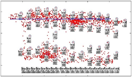
As shown in the figure, the facial photos are clearly separated into two portions. The upper section depicts a face with a closed mouth, whereas the lower part depicts a face with an open mouth. This difference can be explained by the novel technique that implicitly favours natural clusters in the data while attempting to retain the neighbourhood and non-neighbourhood features in the embedding. In the reduced representation space, it brings adjacent and non-neighbouring points in ambient space closer and farther, respectively. The bottom images correspond to locations along the top path (connected by a blue solid line), exhibiting stance variability with a particular facial expression.

6.3. Experiment on the ORL face database

ORL consists of a total of 400 facial images of 40 people (10 samples per person). The people in the set vary in terms of age, gender, and race. The photos were taken at various periods and feature a variety of expressions (open or closed eyes, smiling or non-smiling) and facial characteristics (with glasses or without glasses). For certain tilting and rotation of the faces, the photos were obtained with a tolerance of up to 20 degrees. This database is a widely used standard database.

Before conducting the experiment, we performed data processing similar to that in NPE. The original images were scaled and oriented in such a way that the two eyes would be aligned in the same place. Then, the final image was cropped to match the facial areas. In all of the experiments, the size of each cropped image was 32 × 32 pixels, with 256 grey levels per pixel.

6.3.1. Embedding structure in the low-dimensional space

The aim of our algorithm is to separate non-neighbouring data points as far as possible while preserving the neighbourhood relationship between neighbouring data points in low-dimensional space. Figure 2 presents the distribution of the data points in 2D embedding space described by the first two coordinates of NPE and our novel algorithm. The two figures have the same coordinate scale. Clearly, the degree of dispersion of the data points in the left figure is greater than those in the right figure. This finding proves the ability of the NNNPE to separate the non-neighbouring data points in contrast to the NPE. Moreover, as shown in the figure, each point (individual) represents an overlap of ten data points (facial images) because the location is extremely close to one another, such as the point marked by a circle in the figure. The local property is both preserved by the NPE and the NNNPE, which means that any data point can be represented as a linear combination of its neighbours. Then, the distribution of the 10 neighbouring data points is displayed in a coordinate figure with the same scale. Clearly, the distribution of the 10 neighbouring data points in the left figure is closer than that of the right figure. Thus, the NNNPE can preserve the neighbourhood structure better than the NPE. The results also have a similar manifold structure. Figure 3 presents an order of facial images according to abscissa sorting of 10 data points included in the circle in Figure 2. This scenario represents a particular mode of variability in an individual pose.

Figure 2. Distribution of data points in 2D spaces mapped using NPE and NNNPE. Right figure: NPE; left figure: NNNPE.

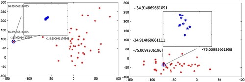
Figure 3. Manifold structure of points marked by a circle according to the order of abscissa. Top: NNNPE; bottom; NPE.

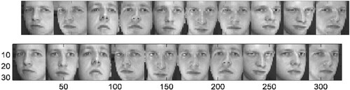
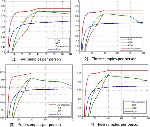
Figure 4. Recognition rate with different dimensionalities and varied numbers of training samples on the ORL dataset.

6.3.2. Face recognition by using NNNPE

 Table 1 shows the best outcomes in the ideal subspace and the appropriate dimensions for each approach. Our innovative method outperforms the competition in all situations. LDA outperforms NPE, but both methods are superior to PCA. Moreover, the optimal dimensionalities obtained by our novel algorithm, along with those of NPE and LDA, are much lower than those obtained by PCA. The average detection time of NNNPE is 1 ms, and the training time is less than 60 s.

Table 1. Performance comparison on the ORL dataset.

Method	2 Train	3 Train	4 Train	5 Train
Baseline	66.2% (1024)	75.4% (1024)	82.0% (1024)	85.9% (1024)
Eigenface	70.44% (80)	78.58% (100)	83.91% (100)	87.54% (100)
Fisherface	79.92% (39)	87.11% (39)	91.13% (39)	93.31% (39)
NPE	80.05% (39)	87.14% (40)	91.23% (39)	93.73% (40)
Our algorithm	82.83% (39)	90.76% (39)	94.40% (39)	96.52% (39)

Table 2. Performance of AlexNet on the ORL dataset.

Epoch method	3000	8000	13,000	20,000
CNN	20.1%	73.7%	92.2%	98.75%

6.3.3. Face recognition based on CNN

A deep learning algorithm is used to train the face recognition model. Even with the use of the earliest image classification model, AlexNet (Krizhevsky et al., 2017), the recognition accuracy is higher than our proposed NNNPE method. Furthermore, in the face recognition task in more complex scenes, the ability of deep learning algorithms is much higher than manifold learning. However, the algorithm proposed in this research is still valuable because manifold learning has good interpretability and offers a reference value in scenarios with strict interpretability requirements. Many scholars are currently attempting to study the interpretability of deep learning algorithms from the perspective of manifold structures.

7. Conclusion

This study introduced a new linear dimensionality reduction approach named NNPE. This algorithm is inspired by the principles of the NPE, LLE, and LDA algorithms and by the MML metric learning method.

This research also explored the connection between LML and MML, both of which have similar locality-preserving properties. In contrast to the nonlinear LLE method, which is defined solely by the training samples, LML and MML can be defined anywhere (and thus on novel test data points). Despite being a linear algorithm, our method can identify the nonlinear structure of the data manifold. Furthermore, the novel algorithm has globalist-preserving properties, which allows non-neighbouring data points to be separated as far as possible in low-dimensional space. The improved performance of our algorithm over other linear dimensionality reduction methods was demonstrated through experiments.

The main idea behind the current work may also be applied to other algorithms (e.g. LPP), which represents the linearisation of nonlinear algorithms. We aim to propose a general framework with this idea in the future. In addition, the NNNPE algorithm proposed in this paper preserves the non-nearest neighbour relationship between samples. When the sample size is larger than a certain level, it becomes difficult to preserve the non-neighbour relationship between all samples, and these problems need to be further explored.

Disclosure statement

No potential conflict of interest was reported by the author(s).

Additional information

Funding

This work is supported by the National Natural Science Foundation of China (NSFC) [grant number 61972187], Natural Science Foundation of Fujian Province, China [grant number 2022J01119], and Fujian Province Young and Middle-aged Teacher Education Research Project [grant number JAT200004]. Open Project of Fujian Provincial Key Laboratory of Information Processing and Intelligent Control (Minjiang University) [grant number MJUKF-IPIC202202].

References

- Baldi, P. (2012). Autoencoders, unsupervised learning, and deep architectures. Proceedings of ICML workshop on unsupervised and transfer learning, pp. 37–49. https://proceedings.mlr.press/v27/baldi12a/baldi12a.pdf.
- Belhumeur, P., Hespanha, J., & Kriegman, D. (1997). Eigenfaces vs. fisherfaces: Recognition using class specific linear projection. IEEE Transactions on Pattern Analysis and Machine Intelligence, 19(7), 711–720. https://doi.org/10.1109/34.598228
- Belkin, M., & Niyogi, P. (2001). Laplacian eigenmaps and spectral techniques for embedding and clustering. Proceedings of the 14th International Conference on Neural Information Processing Systems (NIPS 2001). https://doi.org/10.7551/mitpress/1120.003.0080.
- Bellet, A., Habrar, A., & Sebban, M. (2013). A survey on metric learning for feature vectors and structured data. arXiv Preprint ArXiv:1306.6709. https://arxiv.53yu.com/pdf/1306.6709.pdf
- Brahma, P. P., Wu, D., & She, Y. (2015). Why deep learning works: A manifold disentanglement perspective. IEEE Transactions on Neural Networks and Learning Systems, 27(10), 1997–2008. https://doi.org/10.1109/TNNLS.2015.2496947
- Cai, D., He, X., & Han, J. (2007). Isometric projection. Proceedings of the 22nd AAAI Conference on Artificial Intelligence, pp. 528–533. https://www.aaai.org/Papers/AAAI/2007/AAAI07-083.pdf.
- Chang, X., Nie, F., Wang, S., Yang, Y., Zhou, X., & Zhang, C. (2015). Compound rank-k projections for bilinear analysis. IEEE Transactions on Neural Networks and Learning Systems, 27(7), 1502–1513. https://doi.org/10.1109/TNNLS.2015.2441735
- Donoho, D. L., & Grimes, C. (2003). Hessian eigenmaps: Locally linear embedding techniques for high-dimensional data. Proceedings of the National Academy of Sciences, 100(10), 5591–5596. https://doi.org/10.1073/pnas.1031596100
- He, K., Zhang, X., Ren, S., & Sun, J. (2016). Deep residual learning for image recognition. Proceedings of the IEEE Conference on Computer Vision and Pattern Recognition, pp. 770–778. https://openaccess.thecvf.com/content_cvpr_2016/papers/He_Deep_Residual_Learning_CVPR_2016_paper.pdf.
- He, X., Cai, D., Yan, S., & Zhang, H.-J. (2005). Neighborhood preserving embedding. Tenth IEEE International Conference on Computer Vision (ICCV’05), 2, 1208–1213. https://doi.org/10.1109/iccv.2005.167
- He, X., & Niyogi, P. (2003). Locality preserving projections. Proceedings of the 16th International Conference on Neural Information Processing Systems (NIPS 2003), pp. 153–160. https://proceedings.neurips.cc/paper/2003/file/d69116f8b0140cdeb1f99a4d5096ffe4-Paper.pdf.
- Krizhevsky, A., Sutskever, I., & Hinton, G. E. (2017). Imagenet classification with deep convolutional neural networks. Communications of the ACM, 60(6), 84–90. https://doi.org/10.1145/3065386
- Pehlevan, C., & Chklovskii, D. (2015). A normative theory of adaptive dimensionality reduction in neural networks. Proceedings of the 28th International Conference on Neural Information Processing Systems (NIPS 2015). https://doi.org/10.48550/arXiv.1511.09426.
- Roweis, S. T., & Saul, L. K. (2000). Nonlinear dimensionality reduction by locally linear embedding. Science, 290(5500), 2323–2326. https://doi.org/10.1126/science.290.5500.2323
- Schmidhuber, J. (2015). Deep learning in neural networks: An overview. Neural Networks, 61, 85–117. https://doi.org/10.1016/j.neunet.2014.09.003
- Sumithra, V., & Surendran, S. (2015). A review of various linear and non linear dimensionality reduction techniques. International Journal of Computer Science and Information Technology, 6, 2354–2360. https://citeseerx.ist.psu.edu/viewdoc/download?doi=10.1.1.735.8417&rep=rep1&type=pdf
- Tenenbaum, J. B., Silva, V. d., & Langford, J. C. (2000). A global geometric framework for nonlinear dimensionality reduction. Science, 290(5500), 2319–2323. https://doi.org/10.1126/science.290.5500.2319.
- Turk, M., & Pentland, A. (1991). Eigenfaces for recognition. Journal of Cognitive Neuroscience, 3(1), 71–86. https://doi.org/10.1162/jocn.1991.3.1.71
- Van Der Maaten, L., Postma, E., & Van den Herik, J. (2009). Dimensionality reduction: A comparative. Journal of Machine Learning Research, (10), 66–71. https://members.loria.fr/moberger/Enseignement/AVR/Exposes/TR_Dimensiereductie.pdf.
- Wang, J., He, H., & Prokhorov, D. V. (2012). A folded neural network autoencoder for dimensionality reduction. Procedia Computer Science, 13, 120–127. https://doi.org/10.1016/j.procs.2012.09.120
- Xiang, S., Nie, F., & Zhang, C. (2008). Learning a mahalanobis distance metric for data clustering and classification. Pattern Recognition, 41(12), 3600–3612. https://doi.org/10.1016/j.patcog.2008.05.018
- Yan, C., Chang, X., Luo, M., Zheng, Q., Zhang, X., Li, Z., & Nie, F. (2020). Self-weighted robust LDA for multiclass classification with edge classes. ACM Transactions on Intelligent Systems and Technology, 12(1), 1–19. https://doi.org/10.1145/3418284
- Yang, B., Xiang, M., & Zhang, Y. (2016). Multi-manifold discriminant Isomap for visualization and classification. Pattern Recognition, 55, 215–230. https://doi.org/10.1016/j.patcog.2016.02.001
- Zhang, Y., Zhang, Z., Qin, J., Zhang, L., Li, B., & Li, F. (2018). Semi-supervised local multi-manifold isomap by linear embedding for feature extraction. Pattern Recognition, 76, 662–678. https://doi.org/10.1016/j.patcog.2017.09.043
- Zhang, Z., & Zha, H. (2004). Principal manifolds and nonlinear dimensionality reduction via tangent space alignment. SIAM Journal on Scientific Computing, 26(1), 313–338. https://doi.org/10.1137/s1064827502419154
- Zheng, Y., Tang, Y., Fang, B., & Zhang, T. (2012). Orthogonal isometric projection. Proceedings of the 21st International Conference on Pattern Recognition (ICPR2012), pp. 405–408. https://projet.liris.cnrs.fr/imagine/pub/proceedings/ICPR-2012/media/files/0480.pdf.
- Zhu, X., Huang, Z., Shen, H. T., Cheng, J., & Xu, C. (2012). Dimensionality reduction by mixed kernel canonical correlation analysis. Pattern Recognition, 45(8), 3003–3016. https://doi.org/10.1016/j.patcog.2012.02.007