Business process recommendation method based on cost constraints

ABSTRACT

Business process recommendation can be used to simplify the working procedures of enterprises, avoid unnecessary expenses, and promote the development of enterprises. In the process of process recommendation, there are a lot of activities that are similar in structure and difficult to choose. Here, a process recommendation method based on cost constraints is proposed to solve the problem of difficult to distinguish similar processes. First, the business process is transformed into a labelled Petri net, and the execution probability of each transition is calculated according to the business process log. Then, the matrix used to represent Petri nets is constructed according to the adjacent relationship between transitions, and the matrix is made into the same dimension, and the similarity between matrices is calculated by biggest–smallest approach degree, and the set of Petri nets with similar structure is established. Finally, a cost constraint-based process recommendation method is proposed to find lower service cost items in similar process sets. In the experimental part, the feasibility of the method is compared and verified.

KEYWORDS:

• Cost constraint
• similarity
• business process

1. Introduction

In the past decades, the application fields of business processes have been expanding, such as intelligent financial management (Shao et al., 2021), underwater sensor networks (Wu et al., 2021), intelligent manufacturing systems (Fu et al., 2021), and robotic mission planning. Enterprises are also constantly innovating, and the scale of business processes of enterprises is constantly expanding, especially large enterprises may generate hundreds of business processes. This makes enterprises face a series of new challenges in process analysis, process management, process retrieval, and process recommendation. For example, in the aspect of process management, a series of process model libraries are established to better manage the process. In terms of process retrieval and process recommendation, in order to retrieve effective process models from the process model library for process recommendation, a corresponding model retrieval mechanism is established. The implementation of these aspects requires the similarity calculation of the process model. Therefore, similarity calculation is an important solution to efficiently solve business process problems.

At present, due to the different needs of users, the calculation basis of similarity is also different, which can be roughly divided into three categories (Dijkman et al., 2011): node matching similarity, structural similarity, and behavioural similarity.

Node matching is usually to map the node labels in two process models to calculate similarity. Dijkman et al. (2011) analysed process model similarity from five perspectives, namely, syntax, semantics, attributes of node labels, and node types and node contexts. Ehrig et al. (2007) measured similarity by transforming Petri nets into Semantic Business Process Models (SBPMs). This method does not consider the structure and behaviour of the process, resulting in inaccurate similarity results. Bergmann and Gil (2014) proposed a graph-based semantic workflow similarity measure and combined with cases to improve the traditional graph similarity algorithm, but the retrieval performance is not very high as the number of cases increases.

Most of the structural similarity measurement methods convert business processes into graphs or trees to calculate edit distance and measure the similarity between processes. Dijkman et al. (2009) used graph edit distance to measure the similarity between two processes, i.e. the minimum cost required to transform one graph into another, but cannot distinguish parallel relationships. Zhou et al. (2019) first constructed weighted business process graph, and then used the weighted graph edit distance to measure business process similarity, which can distinguish parallel relationships. Jia et al. (2012) measured the similarity by the tree edit distance between the two trees. Automata can be represented as directed graphs, and Wombacher and Rozie (2006) analysed the structural similarity of workflows from the perspective of automata. Bae et al. (2007) gave the concept of a process dependency graph and transformed this graph into a process matrix to measure the distance between processes.

For behavioural similarity, many methods are currently proposed to calculatebehavioural similarity. Wang et al. (2010) studied the process similarity problem based on PTS, but divided the sequence into cyclic and acyclic structures to calculate the similarity, which destroyed the semantics of the complete sequence. Dong et al. (2014) proposed to use the complete firing sequences to calculate the process similarity for the loop structure problem in Wang et al. (2010), which can effectively deal with the loop structure, but the concurrent structure needs to be listed one by one. Wang et al. (2013) constructed an SSDT matrix according to the shortest succession distance between task in the process, and calculated the similarity by dividing the number of the same elements in the matrix by the total number, which can deal with various structures, but cannot be used for processes index. Zha et al. (2010) measure process similarity according to adjacent relations between activities and can deal with loop structures, but are insensitive to non-free choice structures and ignore the importance of adjacent relations. Yin et al. (2015) added important coefficients to measure similarity based on Zha et al. (2010). Weidlich et al. (2010) extended the adjacent relations of activities, proposed the concept of behaviour profile, and calculated the process similarity according to the behaviour relationship, but it has limitations in the processing of hidden transition, and it is difficult to distinguish between similar structures, that is, it is not easy to retrieve. Facing the problem of process retrieval with similar structures, people hope to find a business process that meets the requirements and conditions, rather than re-develop the process by themselves. At present, most of the process retrieval is to retrieve multiple processes with similar structure, and does not consider variable constraints, such as service cost, and different service quality corresponds to different service cost. For processes that are structurally similar and indistinguishable, people prefer to choose business processes with lower costs. Therefore, this paper analyses and recommends business processes from the perspective of cost constraints.

As the premise of process recommendation, process similarity calculation either only considers process behaviour, or only considers the control flow structure of the process, and does not consider the data flow of the process, that is, the occurrence of actual activities. Based on this, this paper proposes a process similarity calculation method by synthesising the structure, behaviour and activities of the process, and adds cost constraints to recommend the process.

The main contributions of this paper are as follows:

1. Establish a process matrix with execution probability based on Petri net, and co-dimensionalise the matrix, describe the similarity between two processes through the maximum and minimum closeness, and establish a process set with similar structure;

2. Propose a process recommendation method based on cost constraints, and find out the business process with lower service cost in the process set for recommendation.

The structure of the paper is as follows: Section 2 introduces a motivation example, Section 3 gives the basic concepts, and Section 4 introduces the method of calculating similarity between processes. Section 5 describes the cost-based process recommendation algorithm, Section 6 experimental analysis, Section 7 conclusions and future directions.

2. Motivation

Taking the three bank loan processes $N_1$, $N_2$ and $N_3$ in Figure 1 as an example, analyse the similarity of $N_1$, $N_2$ and $N_3$ from the perspective of process behaviour.

Figure 1. Bank loan process.

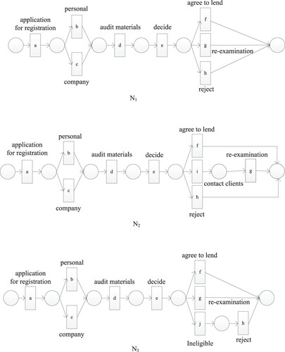
The similarity between two processes is calculated according to the transition adjacency relation proposed by Zha et al. (2010). The transition adjacency sets of $N_1$, $N_2$ and $N_3$ are respectively $\begin{array}{rl}TA{R}_1& =\left\{ab,ac,bd,cd,de,ef,eg,eh\right\},\end{array}$ $\begin{array}{rl}TA{R}_2& =\left\{ab,ac,bd,cd,de,ef,ei,eh,ig\right\},\end{array}$ $\begin{array}{rl}TA{R}_3& =\left\{ab,ac,bd,cd,de,ef,eg,ej,jh\right\},\end{array}$

According to the similarity formula $sim\left(N_1,N_2\right)=\frac{|TA{R}_1\cap TA{R}_2|}{|TA{R}_1\cup TA{R}_2|}$, we can get $sim\left(N_1,N_2\right)=sim\left(N_1,N_3\right)=\mathrm{0.7.}$ At this time, the structure of the process is similar, and the similarity between $N_1$ and $N_2$ and the similarity between $N_1$ and $N_3$ cannot be distinguished according to the transition adjacency relationship, that is, further process recommendation cannot be performed. We improve the calculation method of process similarity, first analyse the activity execution probability, and establish a process matrix, use the concept of closeness in fuzzy mathematics to measure the similarity of two processes, and construct a process set with similar structure, and then a cost constraint-based process recommendation method is proposed to find out the business process with lower service cost in the process set, that is, the business process we want to recommend.

3. Basic concept

The establishment of business process model is crucial to the realisation of process recommendation. There are many modelling notations such as Event-Driven Process Chaining (EPC) (Van der Aalst, 1999), UML Activity Diagram (Eshuis & Wieringa, 2004), Business Process Modeling Notations (BPMN) (Weske, 2019) and Petri Nets (Cheng et al., 2014), by comparing, this paper uses Petri net to represent the business process model. At present, Petri nets have been widely used in intelligent manufacturing systems, communication and artificial intelligence, etc. Different forms of model expansion are carried out on the basis of retaining the basic Petri net model structure and representation method. The process modelling results are easier to understand, such as the extension of the transition connotation in the Petri net to obtain a Petri net with labels, which is defined as follows:

Definition 3.1

((Labelled Petri Net) (Wang et al., 2021)): A 5-tuple $N=\left(P,T,F,\mathrm{\Phi },\lambda \right)$ that satisfies the following conditions is called a labelled Petri net:

1. $P\cup T\ne \mathrm{\varnothing }$;

2. $P\cap T=\mathrm{\varnothing }$;

3. $F\subseteq \left(P\times T\right)\cup \left(T\times P\right)$;

4. $\mathrm{\Phi }$ is the set of active labels for transitions;

5. $\lambda :T\to \mathrm{\Phi }$ is a function of assigning labels to transitions;

where, P is the place set, T is the transition set, and F is the flow relation.

Definition 3.2

((Trace, Event Log) (Fang et al., 2020)): Let $\sum$ be the active transition set of transitions, then the active label sequence is called trace$\sigma \in \sum ^{\ast }$; $L\in B\left(\sum ^{\ast }\right)$ is the multi-set of traces, called the event log, in short, the active labels in the trace only the name, while the active label in the log contain timestamps, resources, etc.

During the actual execution of the business process, some activities may be easy to perform, and others may not occur. The actual implementation of the net $N_1$ of Figure 1 is shown in Table 1.

Table 1. Activity performance.

trace	frequency
abdef	240
abdeg	135
abdeh	45
acdef	120
acdeg	45
acdeh	15
acdgf	3

Definition 3.3

(Activity execution probability): Let N be a labelled Petri net, L is the trace set of the event log, which contains $\mathrm{K}$ traces in total, and the execution probability $\rho$ of each activity t in N is the participation rate of each activity in the event log, that is $\rho \left(t\right)=\frac{|t|}{\mathrm{K}}$, where $|t|$ is the number of occurrences of t in the trace.

Definition 3.4

(Low Frequency Sequence): Let L be the event log, which contains K traces in total. For any trace$l\in L$, the frequency of occurrence in the event log is $\kappa$, then the occurrence frequency of this trace is $\frac{\kappa }{\mathrm{K}}$, If the frequency of occurrence is lower than a given threshold $\xi$, the trace is a low frequency sequence.

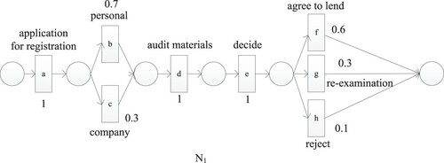
Let $\xi \text{ = }0.01$, and the occurrence frequency of trace acdgf is $\frac{3}{600}<0.01$, which is a low-frequency sequence. At this time, preprocessing is performed to delete it. Then combine Figure1 and Table 1 to get the execution probability of each activity in the net $N_1$, such as $\rho \left(a\right)=\frac{600}{600}=1$. The execution probability graph of net $N_1$ is shown in Figure 2.

Figure 2. Petri net with execution probability.

Definition 3.5

(Adjacent Activity): In the process model, $x,y\in T$, $x,y$ is the adjacent activity if and only if there is an occurrence sequence $\theta =t_1,t_2,\dots ,t_n$, such that $t_i=x$, $t_{i+1}=y$, where $i\in \left\{1,2,\dots ,n-1\right\}$.

For example, the adjacent activities in $N_1$ are ab, ac, bd, cd, etc.

Definition 3.6 (Process Matrix): Let N be a labelled Petri net, and the process matrix NM of N is as follows: (1) $NM\left(i,j\right)=\{\begin{array}{c}\rho \left(t_j\right),t_i\text{and}\begin{array}{c}{t}_j\text{are adjacent activities}\end{array}\\ 0,\text{otherwise}\end{array}$(1) For example, $NM\left(a,b\right)=\rho \left(b\right)=0.7$, $NM\left(b,d\right)=\rho \left(d\right)=1$ in $N_1$, the process matrix of $N_1$ is shown in Table 2. According to the actual situation, the process matrix of $N_2$ and $N_3$ can be obtained in the same way, as shown in Tables 3 and 4.

Table 2. Process matrix for N₁.

	a	b	c	d	e	f	g	h
A	0	0.7	0.3	0	0	0	0	0
B	0	0	0	1	0	0	0	0
c	0	0	0	1	0	0	0	0
d	0	0	0	0	1	0	0	0
e	0	0	0	0	0	0.6	0.3	0.1
f	0	0	0	0	0	0	0	0
g	0	0	0	0	0	0	0	0
h	0	0	0	0	0	0	0	0

Table 3. Process matrix for N₂.

	a	b	c	d	e	f	g	h	i
a	0	0.5	0.5	0	0	0	0	0	0
b	0	0	0	1	0	0	0	0	0
c	0	0	0	1	0	0	0	0	0
d	0	0	0	0	1	0	0	0	0
e	0	0	0	0	0	0.4	0	0.1	0.5
f	0	0	0	0	0	0	0	0	0
g	0	0	0	0	0	0	0	0	0
h	0	0	0	0	0	0	0	0	0
i	0	0	0	0	0	0	1	0	0

Table 4. Process matrix for N₃.

	a	b	c	d	e	f	g	h	j
a	0	0.6	0.4	0	0	0	0	0	0
b	0	0	0	1	0	0	0	0	0
c	0	0	0	1	0	0	0	0	0
d	0	0	0	0	1	0	0	0	0
e	0	0	0	0	0	0.3	0.1	0	0.6
f	0	0	0	0	0	0	0	0	0
g	0	0	0	0	0	0	0	0	0
h	0	0	0	0	0	0	0	0	0
j	0	0	0	0	0	0	0	1	0

Observing the three process matrices, it is found that the dimensions of the matrices are different, so to compare the similarity of the two processes through the process matrix, the process matrix needs to be co-dimensionalised.

Definition 3.7 (Homodimensionalisation of Process Matrix): Let $N_1$ and $N_2$ be two labelled Petri net processes, $N{M}_1$ and $N{M}_2$ are corresponding process matrices, $DN{M}_1$ and $DN{M}_2$ are homodimensional process matrices, defined as follows:

1. $DN{M}_1$ and $DN{M}_2$ are $n\times n$ matrices, where $n=|T_1\cup T_2|$;

2. The matrix $DN{M}_1$ has the same row and column activity names as $DN{M}_2$, which is the union of the $N_1$ and $N_2$ activity names, $T_1\cup T_2=\left\{a_1,a_2,\dots ,a_n\right\}$;

3. $DN{M}_1\left(i,j\right)$ and $DN{M}_2\left(i,j\right)$ are the elements of the i-th row and the j-th column of the matrices $DN{M}_1$ and $DN{M}_2$, respectively. The calculation formula is as follows: (2) $\begin{array}{rl}\text{DN}{\text{M}}_1\left(i,j\right)& =\{\begin{array}{c}N{M}_1\left(i,j\right),a_i,a_j\in T_1\\ \text{0,otherwise}\end{array}\end{array}$(2) (3) $\begin{array}{rl}\text{DN}{\text{M}}_2\left(i,j\right)& =\{\begin{array}{c}N{M}_2\left(i,j\right),a_i,a_j\in T_2\\ 0,\text{otherwise}\end{array}\end{array}$(3)

For example, the process matrices of $N_1$, $N_2$ and $N_3$ are co-dimensionalised to obtain Tables 5–7.

Table 5. Homogeneous matrix of N₁.

	a	b	c	d	e	f	g	h	i	j
A	0	0.7	0.3	0	0	0	0	0	0	0
b	0	0	0	1	0	0	0	0	0	0
c	0	0	0	1	0	0	0	0	0	0
d	0	0	0	0	1	0	0	0	0	0
e	0	0	0	0	0	0.6	0.3	0.1	0	0
f	0	0	0	0	0	0	0	0	0	0
g	0	0	0	0	0	0	0	0	0	0
h	0	0	0	0	0	0	0	0	0	0
i	0	0	0	0	0	0	0	0	0	0
j	0	0	0	0	0	0	0	0	0	0

Table 6. Homogeneous matrix of N_2.

	a	b	c	d	e	f	g	h	i	j
a	0	0.5	0.5	0	0	0	0	0	0	0
b	0	0	0	1	0	0	0	0	0	0
c	0	0	0	1	0	0	0	0	0	0
d	0	0	0	0	1	0	0	0	0	0
e	0	0	0	0	0	0.4	0	0.1	0.5	0
f	0	0	0	0	0	0	0	0	0	0
g	0	0	0	0	0	0	0	0	0	0
h	0	0	0	0	0	0	0	0	0	0
i	0	0	0	0	0	0	1	0	0	0
j	0	0	0	0	0	0	0	0	0	0

Table 7. Homogeneous matrix of N_3.

	a	b	c	d	e	f	g	h	i	j
a	0	0.6	0.4	0	0	0	0	0	0	0
b	0	0	0	1	0	0	0	0	0	0
c	0	0	0	1	0	0	0	0	0	0
d	0	0	0	0	1	0	0	0	0	0
e	0	0	0	0	0	0.3	0.1	0	0	0.6
f	0	0	0	0	0	0	0	0	0	0
g	0	0	0	0	0	0	0	0	0	0
h	0	0	0	0	0	0	0	0	0	0
i	0	0	0	0	0	0	0	0	0	0
j	0	0	0	0	0	0	0	1	0	0

4. Similarity between business processes

Nearness degree is the degree of similarity between fuzzy sets described in fuzzy mathematics (Xie & Liu, 2013). This paper adopts the concept of nearness degree to measure the degree of similarity between business processes.

Definition 4.1

(Nearness Degree): $\sigma \left(A,B\right)$is the nearness degree of A and B, iff

1. $\sigma \left(A,A\right)=1$;

2. $\sigma \left(A,B\right)=\sigma \left(B,A\right)$;

3. if $A\le B\le C$, then $\sigma \left(A,C\right)\le \sigma \left(A,B\right)\wedge \sigma \left(B,C\right)$.

Definition 4.2

(Proximity Principle): It is assumed that there are m fuzzy subsets $A_1,A_2,\dots ,A_m$ on the universe X to form a standard model library, B is the model to be identified, if there is $k\in \left\{1,2,\dots ,m\right\}$ such that $\sigma \left(A_k,B\right)=\vee \left\{\sigma \left(A_i,B\right)|1\le i\le m\right\}$, then B is said to be the closest to $A_k$, or B into the AK category, this is the proximity principle.

Definition 4.3

(Biggest–Smallest Approach Degree): Let $N_1$ and $N_2$ be two labelled Petri net, the biggest–smallest approach degree of $N_1$ and $N_2$ is defined as (4) ${\sigma }_B\left(N_1,N_2\right)=\frac{2\sum _{i=1}^n\sum _{j=1}^n\left(DN{M}_1\left(i,j\right)\wedge DN{M}_2\left(i,j\right)\right)}{\sum _{i=1}^n\sum _{j=1}^n\left(DN{M}_1\left(i,j\right)+DN{M}_2\left(i,j\right)\right)}$(4) where $DN{M}_1\left(i,j\right)\wedge DN{M}_2\left(i,j\right)=inf\left\{DN{M}_1\left(i,j\right),DN{M}_2\left(i,j\right)\right\}$.

For example, calculate the biggest–smallest approach degree between $N_1$ and $N_2$ and between $N_1$ and $N_3$. $\begin{array}{rl}DN{M}_1\left(i,j\right)\wedge DN{M}_2\left(i,j\right)& =0.5+0.3+1+1+1+0.4+0.1=4.3,\end{array}$ $\begin{array}{rl}DN{M}_1\left(i,j\right)\wedge DN{M}_3\left(i,j\right)& =0.6+0.3+1+1+1+0.3+0.1=4.3,\end{array}$ $\begin{array}{rl}DN{M}_1\left(i,j\right)+DN{M}_2\left(i,j\right)& =0.7+0.3+1+1+1+0.6+0.3+0.1+0.5+0.5+1\\ & +1+1+0.4+0.1+0.5+1=11,\end{array}$ $\begin{array}{rl}DN{M}_1\left(i,j\right)+DN{M}_3\left(i,j\right)& =0.7+0.3+1+1+1+0.6+0.3+0.1+0.6+0.4+1\\ & +1+1+0.3+0.1+0.6+1=11,\end{array}$ $\begin{array}{rl}{\sigma }_{BS}\left(N_1,N_2\right)& ={\sigma }_{BS}\left(N_1,N_3\right)=\frac{2\times 4.3}{11}\approx \mathrm{0.78.}\end{array}$ In addition to the biggest–smallest approach degree, the approach degree includes lattice approach degree, distance approach degree, and minimum approach degree, etc. The calculation methods are as follows (Table 8):

Table 8. Comparison of calculation methods for approach degree.

$\sigma$	${\sigma }_{La}$	${\sigma }_{Da}$	${\sigma }_{Min}$	${\sigma }_{BS}$
N1 N2	0.95	0.73	0.64	0.78
N1 N3	0.95	0.73	0.64	0.78

Lattice approach degree: (5) ${\sigma }_{La}\left(N_1,N_2\right)=\frac{1}{2}\left[N_1\circ N_2+\left(1-N_1\odot N_2\right)\right]$(5) Distance approach degree: (6) ${\sigma }_{Da}\left(N_1,N_2\right)=1-\frac{1}{n}\sum _{i=1}^n\sum _{j=1}^n|DN{M}_1\left(i,j\right)-DN{M}_2\left(i,j\right)|$(6) Minimum approach degree: (7) ${\sigma }_{Min}\left(N_1,N_2\right)=\frac{\sum _{i=1}^n\sum _{j=1}^n\left(DN{M}_1\left(i,j\right)\wedge DN{M}_2\left(i,j\right)\right)}{\sum _{i=1}^n\sum _{j=1}^n\left(DN{M}_1\left(i,j\right)\vee DN{M}_2\left(i,j\right)\right)}$(7) Comparing the four approach degree, $\sigma \left(N_1,N_2\right)=\sigma \left(N_1,N_3\right)$. In order to select the appropriate approach degree to calculate the similarity, we calculate the average value of the four methods to be 0.775. At this time, the biggest–smallest approach degrees are the closest to the average value, so the biggest–smallest approach degrees are selected as the method to calculate the similarity, namely $sim\left(N_1,N_2\right)={\sigma }_{BS}\left(N_1,N_2\right)=\frac{2\sum _{i=1}^n\sum _{j=1}^n\left(DN{M}_1\left(i,j\right)\wedge DN{M}_2\left(i,j\right)\right)}{\sum _{i=1}^n\sum _{j=1}^n\left(DN{M}_1\left(i,j\right)+DN{M}_2\left(i,j\right)\right)}$

Table

Algorithm 1: Process Similarity Algorithm
Input: Two Petri net processes with labels $N_1$ and $N_2$, event logs $L_1$ and $L_2$
Output: Similarity sim of $N_1$ and $N_2$
1.For each $a_i\in T_1$ do
2. $\rho \left(a_i\right)\leftarrow ComputerA\text{ctivity Execution Probability}\left(N_1,L_1,a_i\right)$
3. $N{M}_1\leftarrow Computer\text{ProcessMatrix}\left(N_1\right)$
4. end for
5. $n=\left|T_1\cup T_2\right|$
6. $c_q\in T_1\cup T_2$
7. if $c_i,c_j\in T_1$
8. $DN{M}_1\left(i,j\right)=N{M}_1\left(i,j\right)$
9. else $DN{M}_1\left(i,j\right)=0$
10. end if
11. same as above, calculate Homogenised matrix $DN{M}_2\left(i,j\right)$ of $N_2$
12. $DN{M}_1\left(i,j\right)\wedge DN{M}_2\left(i,j\right)=inf\left\{DN{M}_1\left(i,j\right),DN{M}_2\left(i,j\right)\right\}$
13. $sim\left(N_1,N_2\right)={\displaystyle \frac{2\sum _{i=1}^n\sum _{j=1}^n\left(DN{M}_1\left(i,j\right)\wedge DN{M}_2\left(i,j\right)\right)}{\sum _{i=1}^n\sum _{j=1}^n\left(DN{M}_1\left(i,j\right)+DN{M}_2\left(i,j\right)\right)}}$
14. return $sim\left(N_1,N_2\right)$
15. end

Algorithm 1 calculates the similarity between processes, constructs the process matrix in lines 1–4, co-dimensionalises the process matrix in lines 5–s10, and calculates process similarity in lines 12–13.

For $N_1$, $sim\left(N_1,N_2\right)=sim\left(N_1,N_3\right)$, the optimal process cannot be selected. In order to select the business process with the lowest cost service, this paper proposes a process recommendation method based on cost constraints.

5. Process recommendation method based on cost constraints

In the actual execution process of the process, there may be certain preferences, which make some activities have a high probability of execution, and some activities have a low probability of execution, correspondingly, some paths are frequent sequences, and some paths are infrequent sequences. Since $N_1$ is similar in structure to $N_2$ and $N_3$, and the similarity is the same, in order to distinguish, add a double constraint, that is, the cost constraint, and choose the process with less cost of the two, which is the process we finally choose. Therefore, a process recommendation method based on cost constraints is proposed.

Definition 5.1

(Cost Constraint): The cost constraint is denoted by the interval $[p,q]$, where $p$ and $q$ are non-negative real numbers, and $p\le q$, the length of the cost constraint $[p,q]$ is denoted by $l\left([p,q]\right)=p-q+1$.

Definition 5.2

(Occurring Sequence Set): Let N be a labelled Petri net, the set of all possible occurring sequences from the start node to the target node, denoted as SN.

Definition 5.3

(Frequent Sequence, Sequence Cost): Any occurrence sequence $\theta \in SN$, $w=|\theta |$ represents the length of the occurrence sequence, then the occurrence probability of $\theta$ is $\rho \left(\theta \right)=\prod _{i=1}^w\rho \left[\theta \left(i\right)\right]$, if $\rho \left(\theta \right)\ge \delta$ (threshold), then $\theta$ is called a frequent sequence. Call $\cos t\left(\theta \right)=\sum _{i=1}^w\cos t\left[\theta \left(i\right)\right]$ the cost of the sequence occurrence, where the cost of $\theta \left(i\right)$ is determined by the length of the cost constraint.

Table

Algorithm 2: Process recommendation method based on cost constraints
Input: Process Models N1 and N2
Output: probabilistic cost C
1. $r_1\leftarrow ComputerAll\text{OccurrenceSequence}\left(N_1\right)$
2. $r_2\leftarrow ComputerAll\text{OccurrenceSequence}\left(N_2\right)$
3. $S_1=\mathrm{\varnothing }$
4. for each Occurrence sequence ${\theta }_i\in r_1$ do
5. computer$\rho \left({\theta }_i\right)$
6. if $\rho \left({\theta }_i\right)\ge \delta$
7. add ${\theta }_i$ to $S_1$
8. end if
9. end for
10. for each Occurrence sequence ${\theta }_j\in r_2$ do
11. computer $\cos t\left({\theta }_j\right)$
12. end for
13. for each Occurrence sequence ${\theta }_i\in S_1$ do
14. for each Occurrence sequence ${\theta }_j\in r_2$ do
15.  $dis\tan ce=sed\left({\theta }_i,{\theta }_j\right)$
16.  if $dis\tan ce\le mindis\tan ce$
17.   $mindis\tan ce=dis\tan ce$
18.   Occurrence sequence = ${\theta }_j$
19.  end if
20. end for
21. end for
22. C = $\cos t\left({\theta }_j\right)$*$\rho \left({\theta }_i\right)$

Analysis of Algorithm 2: calculate the probability of occurrence of each occurrence sequence of $N_1$, and determine which sequences are frequent sequences, and the consumption cost of each occurrence sequence of $N_2$ (Algorithm 2: 1–12); Then find the occurrence sequence in $N_2$ that is most similar to the frequent sequence in $N_1$, refer to the calculation method of editing distance in reference (Levenshtein, 1966) and calculate the corresponding consumption cost (Algorithm 2: 13–22).

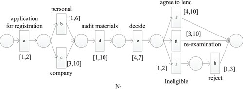
Example: calculate the probabilistic cost of $N_1$ and $N_2$, and the probabilistic cost of $N_1$ and $N_3$ (Figures 3 and 4).

Figure 3. Cost constraint of N_2.

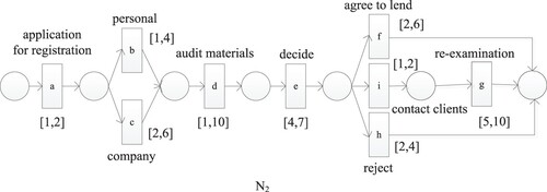
Figure 4. Cost constraint of N_3.

Let $\delta \text{ = }0.15$, the frequent sequence of process$N_1$ is $SN=\left\{abdef,ab\mathrm{deg},acdef\right\}$, and the occurrence sequence of process $N_2$ is most similar to the frequent sequence of process $N_1$, which are $abdef$, $abdeh$, and $acdef$. The consumption costs of these three sequences are 24, 23, and 26, respectively, and the probabilistic cost is $24\times 0.42+23\times 0.21+26\times 0.18=19.59$; The occurrence sequence of process $N_3$ is most similar to the frequent sequence of process N1, which are $abdef$, $ab\mathrm{deg}$, and $acdef$. The consumption costs of these three sequences are 29, 30 and 31, respectively, and the probabilistic cost is $29\times 0.42+30\times 0.21+31\times 0.18=24.06$. Therefore, process $N_2$ is selected as the optimal process of process $N_1$ (Tables 9 and 11).

Table 9. Occurrence sequence and occurrence probability of N_1.

Occurrence sequence	abdef	abdeg	abdeh	acdef	acdeg	acdeh
Occurrence probability	0.42	0.21	0.07	0.18	0.09	0.03

Table 10. Occurrence sequence and consumption cost of N_3.

Occurrence sequence	abdef	abdeig	Abdeh	acdef	acdeig	acdeh
Consumption cost	24	27	23	26	29	24

Table 11. Occurrence sequence and consumption cost of N_3.

Occurrence sequence	abdef	abdeg	Abdejh	acdef	acdeg	acdejh
Consumption cost	29	30	27	31	32	29

6. Experiment and evaluation

6.1. Feasibility analysis of similarity calculation method

The similarity between the processes is calculated by using the current mainstream similarity algorithm, and compared with the calculation method in this paper. The results are shown in Table 12. The result of algorithm 1 is 0.78, and the result of the mainstream algorithm is in the range of 0.7∼0.94, so it is feasible.

Table 12. Algorithm comparison.

The algorithm name	Similarity between N1 and N2
TAR	0.7
TAR++	0.94
WF	0.94
BP	0.75
GED	0.89
SSDT	0.80
Algorithm 1	0.78

6.2 .Time complexity analysis

Algorithm 1 mainly consists of two parts: calculating the homodimension matrix and calculating the similarity. For the homodimension matrix, if the order is n, the complexity of the homodimension matrix is $O\left(n^2\right)$. Similarity calculation involves the calculation of $DN{M}_1\left(i,j\right)\wedge DN{M}_2\left(i,j\right)$. At this time, the time complexity is $O\left(n^2\right)$, so the total time complexity is $O\left(n^2\right)$.

Algorithm 2: The number of occurrence sequences of $N_1$ and $N_2$ is $n_1$ and $m_1$ respectively, and the time required to traverse each occurrence sequence of $N_1$ and $N_2$, and calculate the similarity, and the required time is $O\left(n_1+m_1+n_1\times m_1\right)$.

6.3. Performance evaluation

To evaluate the performance of the algorithm, this paper manually created 200 process models and randomly assigned them into 3 datasets, where dataset 1, dataset 2 and dataset 3 contained 38, 62 and 100 process models, respectively.

We know that the greater the distance between the two processes, the smaller the similarity, and conversely, the smaller the distance, the greater the similarity. The similarity can be converted into distance to check the related properties. The distance between the two processes is $d\left(N_1,N_2\right)=1-sim\left(N_1,N_2\right)$.

1. Non-negativity: the distance between two processes $\begin{array}{rl}& d\left(N_1,N_2\right)=1-sim\left(N_1,N_2\right)=1-\frac{2\sum _{i=1}^n\sum _{j=1}^n\left(DN{M}_1\left(i,j\right)\wedge DN{M}_2\left(i,j\right)\right)}{\sum _{i=1}^n\sum _{j=1}^n\left(DN{M}_1\left(i,j\right)+DN{M}_2\left(i,j\right)\right)},\end{array}$ $\begin{array}{rl}& \because 2\sum _{i=1}^n\sum _{j=1}^n\left(DN{M}_1\left(i,j\right)\wedge DN{M}_2\left(i,j\right)\right)\le \sum _{i=1}^n\sum _{j=1}^n\left(DN{M}_1\left(i,j\right)+DN{M}_2\left(i,j\right)\right),\end{array}$

$\therefore 0\le sim\left(N_1,N_2\right)\le 1$, So it is non-negative.

1. Symmetry: The distance between any two processes is unique, $d\left(N_1,N_2\right)=d\left(N_2,N_1\right)$, that is, the similarity of the two processes is the same, and it has symmetry.

2. Identity: If the two processes are the same, the distance between them is 0, that is, $sim\left(N_1,N_2\right)=1$, which means they are identical.

3. Triangular inequality: Given any three processes N1, N2 and N3 and the distances $d\left(N_1,N_2\right)$, $d\left(N_1,N_3\right)$and $d\left(N_2,N_3\right)$between them, the sum of any two distances is greater than or equal to the third distance, i.e $\begin{array}{rl}& d\left(N_1,N_2\right)+d\left(N_1,N_3\right)\ge d\left(N_2,N_3\right)\end{array}$ $\begin{array}{rl}& d\left(N_1,N_2\right)+d\left(N_2,N_3\right)\ge d\left(N_1,N_3\right)\end{array}$ $\begin{array}{rl}& d\left(N_1,N_3\right)+d\left(N_2,N_3\right)\ge d\left(N_1,N_2\right)\end{array}$

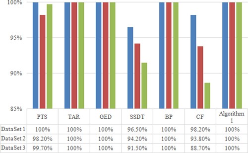
For the verification of the triangle inequality, it is converted into the triangle inequality satisfaction rate for verification. Assuming that there are a total of n process models, three are randomly selected from them, and there are $C_n^3$ways of taking them. If m of them satisfy the triangle inequality, the satisfaction rate of the triangle inequality is $m/C_n^3$.

Comparing the triangular inequality satisfaction rate of mainstream algorithms (Figure 5), it is found that SSDT algorithm and CF algorithm are poor in triangular inequality satisfaction rate, PTS only has some data satisfying triangular inequality, TAR, GED, BP, Algorithm 1 has a better satisfaction rate than PTS, SSDT and CF algorithms.

Figure 5. Comparison of Triangular Inequality Satisfaction Rates.

In addition to satisfying the above four properties, the similarity algorithm in this paper is also related to data and cost (Table 13).

Table 13. Performance comparison of different algorithms.

		Non-			Triangle	Data	Cost
Reference	Classification	negativity	Symmetry	Identity	inequality	correlation	correlation
Ma et al. (2014)	Structure	√	√	√	√	×	×
Ehrig et al. (2007)	Structure	√	√	√	×	×	×
Wombacher and Rozie (2006)	Structure	√	√	√	√	×	×
Yan et al. (2010)	Structure	√	√	√	×	×	×
Liu et al. (2019)	Structure	√	√	√	√	×	×
Weidlich et al. (2010)	Behaviour	√	√	√	√	×	×
Dong et al. (2014)	Behaviour	√	√	√	×	×	×
Chen et al. (2014)	Behaviour	√	√	√	×	×	×
Van der Aalst et al. (2006)	Behaviour	√	×	√	×	×	×
Zha et al. (2010)	Behaviour	√	√	√	√	×	×
Yin et al. (2015)	Behaviour	√	√	√	√	×	×
Dongen et al. (2013)	Behaviour	√	√	√	×	×	×
This article	Structure and	√	√	√	√	√	√
	behaviour

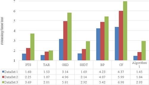
In terms of running time, the running times of different algorithms under several sets of data sets are compared, as shown in Figure 6. It is found that the CF algorithm is time-consuming and has poor running efficiency. The time consumption of algorithm 1 is lower than that of the other algorithms except that of the TAR algorithm.

Figure 6. Comparison of running time.

7. Conclusion and future

In order to simplify the working procedure of enterprises and avoid unnecessary expenses, a process recommendation method based on cost constraint is proposed to solve the existing problems in process retrieval. First, the concept of activity execution probability is given, the execution probability of each activity is calculated, and a process matrix is constructed based on this, and then the similarity between processes is calculated by the biggest–smallest approach degree, and the process set with similar structure is found. Finally, in order to distinguish processes with similar structures, a cost constraint-based process recommendation method is proposed to find out the business processes with lower service cost in the process set. The experimental results show that the similarity calculation is feasible, and the business process with lower cost is recommended. Although the data and cost are considered, the operation efficiency is not worse than other algorithms.

However, the method proposed in this paper requires a process model and a specific process execution log. Compared with other methods, the input conditions are more, and the infrequent behaviour is directly ignored when calculating the execution probability. In the future, in addition to considering infrequent behaviours, further research will be done on the application of process recommendation methods to industrial scenarios to make the methods more adaptable.

Disclosure statement

No potential conflict of interest was reported by the author(s).

Additional information

Funding

This work was supported by the National Natural Science Foundation, China (61572035, 61402011, 61902002), the Natural Science Foundation of Anhui Province, China (2008085QD178), the Key Projects of Natural Science Research in Universities of Anhui Province (KJ2021A0896), the Scientific research project of Anhui Science and Technology University (2021zryb31,880647), the Talent introduction project of Anhui Science and Technology University (XWYJ202107).

References

- Bae, J., Liu, L., Caverlee, J., Zhang, L. J., & Bae, H. (2007). Development of distance measures for process mining, discovery and integration. International Journal of Web Services Research, 4(4), 1–17. https://doi.org/10.4018/jwsr.2007100101
- Bergmann, R., & Gil, Y. (2014). Similarity assessment and efficient retrieval of semantic workflows. Information Systems, 40(MARa), 115–127. https://doi.org/10.1016/j.is.2012.07.005
- Chen, X., Lu, R., Ma, X., & Pang, J. (2014). Measuring user similarity with trajectory patterns: Principles and new metrics. In L. Chen, Y. Jia, T. Sellis, and G. Liu (Eds.), Web technologies and applications (pp. 437–448). Springer International Publishing. https://doi.org/10.1007/978-3-319-11116-2_38
- Cheng, J., Liu, C., Zhou, M., Zeng, Q., & Ylä-Jääski, A. (2014). Automatic composition of semantic web services based on fuzzy predicate petri nets. IEEE Transactions on Automation Science and Engineering, 12(2), 680–689. https://doi.org/10.1109/TASE.2013.2293879
- Dijkman, R., Dumas, M., & García-Bañuelos, L. (2009). Graph matching algorithms for business process model similarity search. In U. Dayal, J. Eder, J. Koehler, and H. A. Reijers (Eds.), Business process management (pp. 48–63). Springer. https://doi.org/10.1007/978-3-642-03848-8_5
- Dijkman, R., Dumas, M., Van Dongen, B., Käärik, R., & Mendling, J. (2011). Similarity of business process models: Metrics and evaluation. Information Systems, 36(2), 498–516. https://doi.org/10.1109/TASE.2010.09.006
- Dong, Z., Wen, L., Huang, H., & Wang, J. (2014). CFS: A behavioral similarity algorithm for process models based on complete firing sequences. In R. Meersman, H. Panetto, T. Dillon, M. Missikoff, L. Liu, O. Pastor, A. Cuzzocrea, and T. Sellis (Eds.), On the move to meaningful Internet systems: OTM 2014 conferences (pp. 202–219). Springer. https://doi.org/10.1007/978-3-662-45563-0_12
- Dongen, B. V., Dijkman, R., & Mendling, J. (2013). Measuring similarity between business process models. In J. Bubenko, J. Krogstie, O. Pastor, B. Pernici, C. Rolland, and A. Sølvberg (Eds.), Seminal contributions to information systems engineering: 25 years of CAiSE (pp. 405–419). Springer. https://doi.org/10.1007/978-3-642-36926-1_33
- Ehrig, M., Koschmider, A., & Oberweis, A. (2007). Measuring similarity between semantic business process models. In APCCM (Vol. 7, pp. 71–80). https://dl.acm.org/doi/10.55551274453.1274465
- Eshuis, R., & Wieringa, R. (2004). Tool support for verifying UML activity diagrams. IEEE Transactions on Software Engineering, 30(7), 437–447. https://doi.org/10.1109/TSE.2004.33
- Fang, H., Li, D., Sun, S., & Fang, X. (2020). Process conformance checking method based on alignment of direct succession relations. Computer Integrated Manufacturing Systems, 26(6), 1473–1482. https://doi.org/10.13196/j.cims.2020.06.004
- Fu, Y., Hou, Y., Wang, Z., Wu, X., Gao, K., & Wang, L. (2021). Distributed scheduling problems in intelligent manufacturing systems. Tsinghua Science and Technology, 26(5), 625–645. https://doi.org/10.26599/TST.2021.9010009
- Jia, N., Fu, X., Huang, Y., Liu, X., & Dai, Z. (2012). Workflow distance metric based on tree edit distance. Journal of Computer Applications, 32(12), 3529–3533. http://www.joca.cn/EN/10.3724SP.J.1087.2012.03529 https://doi.org/10.3724/SP.J.1087.2012.03529
- Levenshtein, V. I. (1966). Binary codes capable of correcting deletions, insertions, and reversals. In Soviet Physics Doklady, 10(8), 707–710. http://mi.mathnet.ru/eng/dan/v163/i4/p845
- Liu, C., Zeng, Q., Duan, H., Gao, S., & Zhou, C. (2019). Towards comprehensive support for business process behavior similarity measure. IEICE TRANSACTIONS on Information and Systems, 102(3), 588–597. https://doi.org/10.1587/transinf.2018EDP7127
- Ma, Y., Zhang, X., & Lu, K. (2014). A graph distance based metric for data oriented workflow retrieval with variable time constraints. Expert Systems with Applications, 41(4), 1377–1388. https://doi.org/10.1016/j.eswa.2013.08.035
- Shao, Q., Yu, R., Zhao, H., Liu, C., Zhang, M., Song, H., & Liu, Q. (2021). Toward intelligent financial advisors for identifying potential clients: A multitask perspective. Big Data Mining and Analytics, 5(1), 64–78. https://doi.org/10.26599/BDMA.2021.9020021
- Van der Aalst, W. M. (1999). Formalization and verification of event-driven process chains. Information and Software Technology, 41(10), 639–650. https://doi.org/10.1016/S0950-5849(99)00016-6
- Van der Aalst, W. M. P., de Medeiros, A. K. A., & Weijters, A. J. M. M. (2006). Process equivalence: Comparing two process models based on observed behavior. In S. Dustdar, J. L. Fiadeiro, & A. P. Sheth (Eds.), Business process management (pp. 129–144). Springer. https://doi.org/10.1007/11841760_10
- Wang, J., He, T., Wen, L., Wu, N., Ter Hofstede, A. H., & Su, J. (2010). A behavioral similarity measure between labeled Petri nets based on principal transition sequences. In OTM Confederated International Conferences “On the Move to Meaningful Internet Systems” (pp. 394–401). Springer. https://doi.org/10.1007/978-3-642-16934-2_27
- Wang, L. L., Fang, X. W., Shao, C. F., & Asare, E. (2021). An approach for mining multiple types of silent transitions in business process. IEEE Access, 9, 160317–160331. https://doi.org/10.1109/ACCESS.2021.312857
- Wang, S., Wen, L., Wei, D. S., Wang, J., & Yan, Z. Q. (2013). SSDT matrix-based behavioral similarity algorithm for process models. Computer Integrated Manufacturing Systems, 19(8), 1822–1831. https://doi.org/10.13196/j.cims.2013.08.023
- Weidlich, M., Mendling, J., & Weske, M. (2010). Efficient consistency measurement based on behavioral profiles of process models. IEEE Transactions on Software Engineering, 37(3), 410–429. https://doi.org/10.1109/TSE.2010.96
- Weske, M. (2019). Business process management architectures. In M. Weske (Ed.), Business process management: Concepts, languages, architectures (pp. 351–384). Springer. https://doi.org/10.1007/978-3-662-59432-2_8
- Wombacher, A., & Rozie, M. (2006). Evaluation of workflow similarity measures in service discovery. In Service-Oriented Electronic Commerce, Proceedings zur Konferenz im Rahmen der Multikonferenz Wirtschaftsinformatik (pp. 20–22). https://dl.gi.de/handle/20.500.12116/24294
- Wu, J., Sun, X., Wu, J., & Han, G. (2021). Routing strategy of reducing energy consumption for underwater data collection. Intelligent and Converged Networks, 2(3), 163–176. https://doi.org/10.23919/ICN.2021.0012
- Xie, J., & Liu, C. (2013). Fuzzy mathematics method and its application. Huazhong University of Sclence & Technology Press.
- Yan, Z., Dijkman, R., & Grefen, P. (2010). Fast business process similarity search with feature-based similarity estimation. In OTM Confederated International Conferences “On the Move to Meaningful Internet Systems” (pp. 60–77). Springer. https://doi.org/10.1007/978-3-642-16934-2_8
- Yin, M., Wen, L. J., Wang, J. M., Xiao, H., Ding, Z., & Gao, X. (2015). Process similarity algorithm based on importance of transition adjacent relations. Computer Integrated Manufacturing Systems, 21(2), 344–358. https://doi.org/10.13196/j.cims.2015.02.007
- Zha, H., Wang, J., Wen, L., Wang, C., & Sun, J. (2010). A workflow net similarity measure based on transition adjacency relations. Computers in Industry, 61(5), 463–471. https://doi.org/10.1016/j.compind.2010.01.001
- Zhou, C., Liu, C., Zeng, Q., Lin, Z., & Duan, H. (2019). A comprehensive process similarity measure based on models and logs. IEEE Access, 7, 69257–69273. https://doi.org/10.1109/ACCESS.2018.2885819