A continual learning framework to train robust image recognition models by adversarial training and knowledge distillation

Abstract

Deep learning has been widely adopted in many image recognition tasks with great success. It has now been applied to conducting tasks on vision-based edge devices with resource limitation. To securely deploy image services on such devices, this work develops a framework to investigate the key issues relate the most to training robust and lightweight models. The primary issue is about safety. It is well known that the deep learning method is vulnerable to well-designed attacks. To meet the challenge of continuously evolving attacks, we develop a new defensive approach that integrates continual learning and adversarial training to improve the defensive model's corruption robustness and structure compactness. This approach adopts the structure of a progressive neural model to establish a robust model over time. The second issue is about how to train a lightweight model. Regarding this, we develop another new knowledge distillation approach that integrates both self-distillation and multi-teacher distillation techniques. With such a specially designed student-teacher learning structure and new loss functions, our approach is thus adaptable to different task situations. To verify the proposed framework, we have conducted a series of experiments to evaluate our approach. The results well confirm its functions and effectiveness.

KEYWORDS:

• Image attack
• deep learning
• adversarial training
• continual learning
• knowledge distillation

1. Introduction

In recent years, running deep learning algorithms with large amounts of data are becoming increasingly popular to achieve various applications. Deep learning has shown superior performance for visual tasks and is now used to train image models for resource-constrained systems. However, to deploy a successful and secure service for such devices, we must tackle the critical issues of training robust and lightweight models. This work presents an enhanced deep learning framework to solve the relevant issues.

The first task is to enhance the robustness of the model. Recent studies find deep learning vulnerable against well-designed input data to train image models, resulting in severe performance problems (Croce & Hein, 2020; Rice et al., 2020; Song et al., 2023). Adversaries can carefully craft imperceptible perturbations that can be injected into clean images to generate misclassified examples (i.e. adversarial examples, AE). Deep neural networks are exposed to the risk of adversarial attacks via the fast gradient sign method (FGSM), projected gradient descent (PGD) attacks, and other attack algorithms (Goodfellow et al., 2015). Adversarial training is often used to defend against the threat of adversarial attacks. However, even though defensive models are effective, most are only defensive against some common attacks rather than the stronger or unseen ones. A defensive method used to prevent existing attacks was, in fact, vulnerable to some new attacks. To enhance the robustness of the models against such unknown/new attacks, researchers have proposed continual learning (CL) as a practical approach (Cossu et al., 2021; Schwarz et al., 2018). It trains a model to achieve a set of sequential tasks from its previous experiences by progressively acquiring, fine-tuning, and transferring knowledge. As is shown, continual learning provides a way to avoid the problem of catastrophic forgetting (Mundt et al., 2023; Pfülb & Gepperth, 2019). Table 1 lists the abbreviations and descriptions used in this work to enhance readability.

Table 1. Abbreviations and their descriptions used in this work.

abbreviation	full text	description
AE	adversarial example	an example of an object capable of deceiving a neural network algorithm
FGSM	fast gradient sign method	a method of generating adversarial examples with a one-step gradient update along the direction of the sign of the gradient
PGD	projected gradient descent	an adversarial attack technique by adding random perturbation to the model gradient to generate the adversarial example
CL	continual learning	a learning concept to learn a model for a set of tasks sequentially without forgetting knowledge obtained from the preceding tasks
KD	knowledge distillation	the process of transferring knowledge from a large model to a smaller one
CPG	compacting, picking and growing	A continual learning method with steps of model compacting, weight picking and model growing
CMAT	continual learning model with adversarial training	the proposed continual learning method with adversarial training
MTKD	multi-teacher knowledge distillation	a knowledge distillation method with multiple teacher models
SMDKD	self multiple teacher knowledge distillation	a multiple teacher knowledge distillation method with self-distillation technique
ResNet	Residual neural network	a deep learning model in which the weight layers learn residual functions with reference to the layer inputs
VGG	Visual Geometry Group	a standard deep Convolutional Neural Network architecture with increased depth to increase the model performance
SGD	stochastic gradient decent	an optimisation algorithm often used in to find the best fit model parameters
SMDKDS	SMTKD with the student as one of the teachers	the proposed knowledge distillation method

The other important work in developing image models is to train lightweight/compacted models with high performance, so the models can be used efficiently to work with different training methods or in resource-constrained devices. As mentioned above, deep neural networks have achieved superior performance on many tasks while relying on deep/wide network architecture with large numbers of layers and parameters to increase the learning capacity. It is thus a challenge to deploy a comprehensive deep model on platforms with limited computation and storage resources for real-time applications (Han et al., 2023; Incel & Bursa, 2023). Various model compression and acceleration techniques have been developed for learning efficient and lightweight deep models, such as network pruning, model quantisation, and knowledge distillation (KD) (Gou et al., 2021). Among those methods, KD has attracted more and more attention from the research community. This knowledge transfer method includes explicitly two models: the pretrained large model as the teacher model and the lightweight model as the student model. The goal is to learn a small student model by transferring knowledge from a pretrained cumbersome teacher model (Hinton et al., 2015). With the distilled knowledge from the teacher model, the student model can usually achieve good performance or even outperform the teacher model.

In this work, we develop a deep learning framework to train robust and lightweight models for image recognition. Our framework has several important contributions. It includes a new adversarial training approach that deliberately integrates continual learning and progressive adversarial training to improve the defensive model's corruption robustness and structure compactness. This proposed approach adopts the CPG structure (compacting, picking and growing) (Hung et al., 2019) as the basic model with the growing and pruning phases for continual learning to perform adversarial training progressively. Our framework also includes a new knowledge distillation approach that integrates both self-distillation and multi-teacher distillation techniques with a specially designed student-teacher learning structure and a new loss function. To verify the advantages of this framework, we have conducted a series of experiments to evaluate the methods and compare them with others. The results confirm the usefulness and effectiveness of the presented approach.

2. Background and related work

As mentioned above, various methods have been proposed to enhance the image recognition models, and their feasibility and performance vary from level to level. Among others, deep learning has been widely used in various domains of image processing and recognition with superior performance. Regarding system robustness and lightweight in image recognition, there are some comprehensive studies categorising works by deep learning from different perspectives (for example, works by Incel and Bursa (2023) and Song et al. (2023)). This study adopts deep learning models as the functional components to build an image recognition system regarding the critical issues of model robustness and compression. In the following subsections, we analyse some of the most relevant works.

2.1. Adversarial training and continual learning

The first concern is with how to construct a robust recognition model. As is known, the small perturbation to AI algorithms (especially deep learning models) can significantly affect the system's performance and even security. Various defense strategies have been proposed to reduce perturbation, such as input noises or attacks (adversarial examples). Researchers have demonstrated how the adversarial examples declined the system performance (Du et al., 2023). Among the studies on building adversarial examples, Szegedy et al. conducted the first work to generate small perturbations on the images to mislead the state-of-the-art deep neural networks with high probability (Szegedy et al., 2014). Then, Goodfellow et al. proposed a fast method called FGSM to generate adversarial examples with a one-step gradient update along the direction of the sign of the gradient (Goodfellow et al., 2015). Through extending FGSM, Kurakin et al. performed a minor change optimisation for multiple iterations to obtain higher attack success rates (Kurakin et al., 2017). Madry et al. also developed an iterative method called PGD attack (Madry et al., 2018). PGD attack starts from a random perturbation in Lp-ball around the input sample to generate the most adversarial example, namely, to find the local maximum loss value of the model.

New methods have been proposed to defend against adversarial examples to enhance model performance. Training with AEs is one of the countermeasures to make neural networks more robust (Aldahdooh et al., 2022; Yuan et al., 2019), and studies have shown that adversarial training can improve the robustness of deep neural networks. For example, Goodfellow et al. included adversarial examples in the training stage (Goodfellow et al., 2015). Yu et al. proposed a method to improve the model robustness by progressively injecting diverse adversarial noises during training (Yu et al., 2021). Liu et al. proposed a strategy that utilised the potential of hidden layers; it can be combined with other adversarial training methods to improve the robustness further (Liu et al., 2021). In a recent application, Ma et al. applied similar training to medical images by searching and adjusting the local decision boundary location (Ma & Liang, 2022). All authors mentioned above generated adversarial examples in every training step and injected them into the training set in various ways. Moreover, Cai et al. proposed a curriculum adversarial method to solve the overfitting problem associated with the above iterative methods (Cai et al., 2018); Zhang et al. also monitored the attack strength with dynamic adversarial training (Zhang et al., 2020).

Tramèr et al. found that the adversarial trained models on the datasets MNIST and ImageNet were more robust to white-box adversarial examples than to the transferred examples (black-box) (Tramèr et al., 2018). However, adversarial examples generated by a neural model often exhibit black-box transferability that misleads other models with the same learning task of different structures. Then, some works focusing on generating more transferable adversarial examples can be roughly classified into four categories: ensemble-model attack, momentum-based attack, input transformation-based attack, and model-specific attack. They can be integrated to achieve even higher transferability.

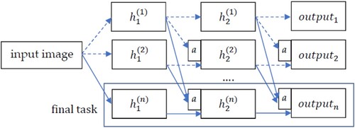
In adversarial training, continual learning is regarded as an effective approach to enhance the model robustness by gradually considering more adversarial examples. In general, CL trains a model to achieve a set of sequential tasks from its previous experiences through progressively acquiring, fine-tuning, and transferring knowledge. CL takes a model pretrained on a source domain, and then the output layer of this model is trained to adapt to the target domain by the fine-tuning technique. Fine-tuning has been proven a useful technique for transfer learning with neural networks. For example, Hinton et al. conducted a pioneer study of transfer learning, which moved from a generative model to a discriminative model (Hinton & Salakhutdinov, 2006). However, their method was unsuitable for multi-task transfer learning because it required a learning method to initialise subsequent models with the experiences of the previous training data. Rusu et al. presented a progressive neural network model to satisfy the needs above (Rusu et al., 2016). Progressive networks retain a pool of pretrained models throughout training and learn lateral connections from these to extract useful features for new tasks. In this way, the network allows prior knowledge to be integrated at each layer of the feature hierarchy. This approach has become popular and adopted to train models for adversarial attacks (for example, works by Liu et al. (2021) and Joseph et al. (2021)). Figure 1 shows the architecture of progressive neural network. Here, h represents the hidden unit, a represents the adaptive layer, and the solid lines indicate the final task of learning gradually from the previous tasks.

Figure 1. Architecture of the progressive neural network.

Though progressive networks have many advantages, their common problem lies in the network size being overly large due to new weights gained from accommodating new knowledge for new tasks. Once the network structure is too large, the corresponding performance might degrade. The PackNet approach was proposed to solve this problem (Mallya & Lazebnik, 2018). This approach can limit and fix the size of each task model through specific rules. Thus, the network architecture can learn the essential weights as much as possible while retaining the memories required by each task within a particular size of the network. Meanwhile, it prioritises tasks according to the complexity of learning so the network can make subsequent tasks better to learn. PackNet can improve the progressive network by considering network compactness, and this approach has been widely used in continual learning applications that often require training with datasets of multiple tasks. However, its major disadvantage is that when the original extensible features of the model were lost, the weights remained constants. Based on PackNet, researchers have proposed a new structure of pack and expand with advantages of unforgettability, compactness and extensibility at the same time. Inspired by this structure, Hung et al. presented a CPG approach for unforgetting continual learning (Hung et al., 2019). CPG can exploit the accumulated knowledge to enhance the new task performance and prune the weights from previous tasks. Though the above approaches have been widely used in various applications (for example, Guo et al. (2023)), they were not used for adversarial training. In this work, we develop a new approach that embeds adversarial training and progressive training into continual learning. The former training generates and injects the increased random perturbation during the model training process; the latter performs compacting, pruning and growing to learn a new task from previous ones. Continuing with the above learning iteration, we can obtain a robust model. For details, see Section 3.2.

2.2. Self distillation and multi-teacher distillation

In addition to the model robustness, the second concern is how to deploy a small model to obtain the same level of performance as a large model. Recently, knowledge distillation has been advocated to enhance the efficiency of image models by exploring different knowledge, different distillation schemes or different teacher-student architectures (Gou et al., 2021). Our goal is to develop lightweight image models. In this subsection, we analyse the most relevant works that adopted the multi-teacher knowledge distillation algorithm and self-knowledge distillation algorithm to train recognition models.

As is known, knowledge distillation has been designed to compress an ensemble of deep neural networks. It is to transfer knowledge from deeper and wider models to shallower and thinner models. The quality of knowledge acquisition and distillation from teacher to student is mainly determined by the architecture of the teacher-student network and the strategy of bridging the gaps between them (Gao et al., 2021; Mirzadeh et al., 2020). To effectively transfer knowledge to student models, a variety of methods have been proposed for a controlled reduction of the model complexity, for example (Crowley et al., 2018; Gao et al., 2021). In recent years, there are also several methods focusing on minimising the structural differences between the student and the teacher models. For example, Nowak and Corso proposed a structure compression method to transfer the knowledge learned by multiple layers to a single layer (Nowak & Corso, 2018). Wang et al. further performed block-wise knowledge transfer from teacher models to student models while preserving the receptive field (Wang et al., 2018). The teacher models were usually ensembles of student models that shared a similar (or the same) structure with each other (Furlanello et al., 2018).

Different from most knowledge distillation studies which considers only one teacher model, You et al. proposed a multi-teacher knowledge distillation technique (You et al., 2017). Using multiple teacher models to jointly train the student model allows the student model to acquire more knowledge from different perspectives. Technically speaking, considering the multi-teacher knowledge distillation, the core of this algorithm is to use many pretrained models as its teachers to assist training the student model, so the accuracy of the student model can be close to the average accuracy of the teacher models, or the student can outperform them. This method can effectively exploit the knowledge in the pretrained models that has been trained with a large amount of data to assist the student model using only a small amount of data. In this way, the student model can extract the knowledge embedded in multiple teacher models to improve its performance further. To evaluate their approach, the authors conducted a set of experiments on CIFAR-10 and CIFAR-100 datasets for testing. Here, three teacher models were used with about 9M parameters in total, and a student model included about 2.5M parameters. The results prove that the student model in both datasets is even more accurate than the best teacher model. More studies on knowledge distillation can be found in the survey work (Gao, 2023; Gou et al., 2021).

One special knowledge distillation method is self-distillation, in which the algorithm mainly uses the same model to play both roles of teacher and student (Gou et al., 2021; Luan et al., 2019). In the absence of a teacher network, the student network extracts knowledge from the deep layers of the network itself and transfers the knowledge to the shallow layers to complete the self-learning process. To be more specific, Zhang et al. proposed a new self-distillation method: the network was divided into several sections, while knowledge from the deeper sections of the network (regarded as the teacher) was distilled into its shallow sections (Zhang et al., 2019a). Under this architecture, the section in the shallowest layer (the student) has the fastest calculation speed and yet the lowest accuracy, while the section in the deepest layer has the slowest calculation speed and the highest accuracy. This architecture was tested on the CIFAR-100 dataset with high accuracy and proved its effectiveness. To improve the above approach further, Luan et al. proposed the multiple self-distillation method with a similar architecture (Luan et al., 2019). In this method, the self-distillation of the shallow section (student model) was enhanced by several deeper sections (teachers). This method has also been tested on the CIFAR-100 dataset, and the results show the accuracy of the student model significantly improved.

Although the multi-teacher knowledge distillation algorithm (MTKD) can effectively obtain knowledge from multiple teacher models to improve the accuracy of the student model, it has to consume a lot of computing resources to train multiple teacher models during the training process. To exploit the advantages of both knowledge self-distillation and multiple teacher distillation techniques, we integrate them in this work to train a student model with a small amount of data. The details are described in Section 3.3.

3. Training robust and lightweight image recognition models

3.1. System framework

Considering the influence of environmental disturbance and resource limitation, this study presents a deep learning framework to develop robust and lightweight image recognition models that can be launched on resource-constrained devices in real time. One possible way to establish such an image training system is to learn an end-to-end model with all relevant functions. However, the trained model cannot be enhanced in part nor studied from different perspectives because the functional structure of a deep learning-based end-to-end model is often difficult to identify clearly. To practically deploy this framework and investigate the relevant issues in detail, we develop two separate modules responsible for the functions of adversarial training and lightweight modelling, respectively. Figure 2 illustrates the outlook of the proposed framework. As shown, the two modules can work either individually or together to achieve the corresponding function. For example, lightweight modelling can be used to compress the model during the iterative training procedure of adversarial training. In this work, we develop and evaluate them separately. This design has several advantages. The modules of adversarial training and lightweight modelling can be constructed using any effective methods available. This way, the system operates flexibly, and the results are transparent and interpretable to system designers and users. This is especially important for continual learning in which the critical parts (model parameters) can be identified, analysed, and improved iteratively.

Figure 2. Proposed framework of training recognition models.

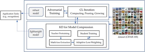
This work describes the two modules (adversarial training and model compression) in turn. The first module includes two parts: an adversarial training algorithm for training the model with random perturbation, and an iteration control algorithm for retraining the model with functions of compacting, pruning and growing the current model. This module is revised and extended from our previous work on adversarial training (Chou et al., 2022). The second module is a knowledge distillation method for model compression. It aims to pretrain a large teacher model and transfer what the teacher model learned to a small student model by aligning their weights. The operational details of the two modules are described in Sections 3.2 and 3.3, respectively.

3.2. Continual learning with adversarial training

As mentioned above, some relevant studies have evaluated the pruning technique and confirmed its use in adversarial training as effective that can reduce the calculation space and obtain better results, e.g. (Madaan et al., 2020; Zhang et al., 2019b). Here in this work, we adopt the structure of progressive neural network as the basis of our model architecture and present Continual Learning Model with Adversarial Training (CMAT), which is an enhanced training approach that integrates the pruning technique into PackNet to improve the performance of defending adversarial attacks. Details are described in the following subsections. How to include perturbations during the iteratively adversarial training procedure (Algorithm 1) and then the steps of packing/pruning and growing in CMAT (Algorithm 2) are described in the following subsections.

3.2.1. Adversarial training with increased data complexity

As indicated in Algorithm 1, the input data are images and the training data X corresponds to class y, following data distribution D, in which $X=\left\{x_1,x_2,x_3,\dots ,x_{|X|}\right\},x\in {\mathbb{R}}^d$, $d$ is the dimension of x and $y$ $\in C$, $C=\left\{c_1,c_2,\dots ,c_{|C|}\right\}$, representing the labels of images. Given task m, the model trained on task m-1 and a set of parameters θ are needed. The perturbation bound ε, the size of the PGD adversary steps s, the max number of iterations $\mathcal{K}$ and learning rate η are pre-defined before adversarial training. During the process of adversarial training, perturbation is an important variable in generating adversarial examples, and the perturbation is updated (increased) by the gradient descent iteratively. The procedure is to increase the data complexity so that the retrained model can be expected to have a better capability of defense. Some studies point out that the complexity of the data is positively correlated with the robustness of the model. Here, we use the PGD algorithm (Algorithm 1) to construct adversarial examples for adversarial training. Before starting the adversarial training, we initialise the set of parameters θ so that the subsequent gradient calculations can be performed. As shown in the figure, there are two loops in this algorithm. The outer loop is to continue the training process for certain iterations; and the inner loop (lines 3-12), to generate perturbations for the adversarial training. To prevent the random perturbation from becoming too large, we adjust the range of perturbation by giving a threshold ε to define the bounds for the perturbation (lines 4-9). Meanwhile, when adding perturbations to the training examples, we specify the number of iterations $\mathcal{K}$ required to generate adversarial examples through the loop. The random uniform distribution (line 4) is used to generate initial perturbations within a defined range.

Once a random perturbation is generated and added to data x (becoming x_adv), we adopt the cross-entropy loss function to guide the training. In this algorithm, ${\mathrm{\nabla }}_{x}L\left(\theta ,x_{\mathrm{adv}},y\right)$ represents the result of the loss function, in which the vector G_adv is obtained based on the model parameters and the disturbed training data (line 7). The gradient vector G_adv contains derivatives of y with respect to x_adv calculated by loss function L. Then, the sign function is used to take the sign of G_adv (i.e. positive or negative). PGD on the negative loss function is a more powerful adversarial technique based on a multi-step variant. The result is multiplied by the step size s to obtain the update based on the size of the PGD adversary steps, which is then added to x_adv to complete the perturbation step of an image (line 8). To avoid perturbation being overly large, the clip functions $\text{clip}\left(x_{\mathrm{adv}},x-ϵ,x+ϵ\right)$ and $\text{clip}\left(x_{\mathrm{adv}},0,1\right)$ are used to define the range to limit the value (lines 9-10). The above steps duly continue for a pre-defined number of iterations for each data example.

After generating the adversarial perturbation, we use the gradient descent method to update the parameters of the model (lines 13-14). During the updating process, the adversarial examples are generated to maximise the loss value: (1) $\begin{array}{r}\mathcal{J}\left(\theta \right)={\mathbb{E}}_{\left(x,y\right)\sim D}\left[\underset{\delta \in S}{max}L\left(\theta ,x_{\mathrm{adv}}=x+\delta ,y\right)\right]\end{array}$(1) Equation (1) obtains a set of allowed perturbations $S\subseteq {\mathbb{R}}^d$ that formalise the manipulative power of the adversary and $\delta \in S$. The classification model, denoted as$\underset{\theta }{\text{ min}}\mathcal{J}\left(\theta \right)$, aims to reduce the loss as much as possible (i.e. to minimise the maximum loss). That is, the adversarial training intends to increase the perturbation (data complexity) by maximising the loss, whereas the goal of the training procedure is to search the suitable network parameters for the model to have better robustness under the strongest pressure of perturbation. The PGD adversarial training is completed after n epochs.

Table

Algorithm 1: CMAT (PGD adversarial training)
Input: Training samples $X$, training sample labels $y$ from the given task $m$ and an original model trained on task $m$−1, the set of model parameters $\theta$, perturbation bound $ϵ$, the size of the PGD adversary steps $s$, the max number of iterations $\mathcal{K}$ and learning rate $\eta$
Output: $\mathrm{ac}{c}_m$
1:	Initialize $\theta$
2:	for epoch $=1\dots N$ do
3:	for min_batch $B$ $\subset$ $X$ do
	# Build $x_{\mathrm{adv}}$ for $x$ $\in$ $B$ with PGD:
	# Assign a random perturbation
4:	$x_{\mathrm{adv}}\leftarrow x+\text{Random}\left(-ϵ,ϵ\right)$
5:	$x_{\mathrm{adv}}\leftarrow \text{clip}\left(x_{\mathrm{adv}},0,1\right)$
6:	for $k=1\dots \mathcal{K}$ do
7:	$G_{\mathrm{adv}}\leftarrow {\mathrm{\nabla }}_{x}L\left(\theta ,x_{\mathrm{adv}},y\right)$
8:	$x_{\mathrm{adv}}\leftarrow x_{\mathrm{adv}}+s\cdot \text{sign}\left(G_{\mathrm{adv}}\right)$
9:	$x_{\mathrm{adv}}\leftarrow \text{clip}\left(x_{\mathrm{adv}},x-ϵ,x+ϵ\right)$
10:	$x_{\mathrm{adv}}\leftarrow \text{clip}\left(x_{\mathrm{adv}},0,1\right)$
11:	$\text{Let}\mathcal{J}\left(\theta \right)={\mathbb{E}}_{\left(x,y\right)\sim D}\left[\underset{\delta \in S}{max}L\left(\theta ,x_{\mathrm{adv}}=x+\delta ,y\right)\right]$
12:	end for
	# Update $\theta$ with stochastic gradient descent:
13:	$G_{\theta }\leftarrow {\mathrm{\nabla }}_{x}L\left(\theta ,x_{\mathrm{adv}},y\right)$
14:	$\theta \leftarrow \theta -\eta \cdot G_{\theta }$
15:	$\text{Let}\underset{\theta }{\text{ min}}\mathcal{J}\left(\theta \right)$
16:	end for
17:	end for

3.2.2. Iteration of compacting, pruning and growing

Following the adversarial training described above, in this section, we present the second part of our CMAT approach that continuously updates the task model through two phases: growing and compacting/pruning. In each phase, the model is retrained by executing the adversarial training procedure (i.e. Algorithm 1) to ensure the performance. Algorithm 2 presents the flow of the major steps of our continual learning with pseudo code.

Before the main flow starts, we perform several preprocessing operations. For this continual learning method, we first divide the task into a set of subtasks (tasks 1∼T) and gradually train the model in sequence. Here, the task is to train an image recognition model, and the task division means to divide the training dataset into subsets by random sampling. We use Algorithm 1 to obtain an initial CMAT model (for task 1) and continuously improve the model to achieve other tasks (i.e. task 2 to the final task T). Also, we specify a targeted accuracy rate tacc_m (determined by a preliminary test) to the current task m, so that the CMAT can accordingly determine whether to expand the model (i.e. the growing phase) or to start pruning (i.e. the compacting-and-pruning phase). To avoid overly enlarging the model and to restrict the model trainer from assigning the required space arbitrarily, we regulate the maximum space of the model by setting the network with a multiplier α. Then, the pruning procedure also constrains the pruning space in which an initial prune ratio p is defined, and the interval of prune ratio v is gradually increased. The details for Algorithm 2 are described below.

Given the initial model trained by the corresponding dataset (for task 1), we perform progressive pruning on the model as described in (Zhu & Gupta, 2018), aiming at eliminating the redundant weights of the model as more as possible while maintaining the same level of performance. Progressive pruning iteratively deposits a part of the model’s weights based on the target pruning ratio specified, and then retrains the model until the pre-defined pruning criterion (e.g. a satisfactory performance or a certain number of iterations) is met. This is to compress the current model to release the redundant space (i.e. memory or model space) of the model’s weights. The reserved weights are fixed during the procedure of model training for subsequent tasks to avoid the forgetting situation.

For task m, a model is trained for this task, and the reserved and released sets of weights are defined as $W_m^T$ and $W_{1:m}^H$, respectively. After the pruning phase, a compacted model is obtained to solve tasks 1 to m, and the reserved weights are represented as $W_{1:m}^H$. The model for each task is built up by the same adversarial training on the corresponding dataset before performing the pruning process, so that the compacted model can learn features of each task. Picking the reserved weights into the next task (line 2), we use the learnable mask S ∈ (0,1)^d with the dimension D of $W_{1:m-1}^H$. The picked weights are represented as $S\odot W_{1:m-1}^H$, in which the symbol $\odot$ is the element-wise product of the 0–1 mask M and as $W_{1:m}^H$. Without losing generality, we adopt the piggyback technique (Mallya & Lazebnik, 2018) to learn a real-valued mask $\hat{S}$, and apply a threshold of binarisation to obtain S. Then, to tackle a new task (i.e. task m), we select a set of weights (called key weights) from the compacted model via the mask and use the expanded weights $W_m^T$ for the new task (line 6). Through backpropagation, the mask S, picked weights, and the additional weights $W_m^T$ are jointly learned on the training data for the new task (line 7). If the performance is not satisfied, the model architecture is expanded by multiplying α (in the growing phase) to include more weights for training (line 5). In other words, other weights, such as the new filters in the convolutional layer and nodes in the fully connected layer, can be used to expand $W_m^T$. Notably, during the task-transfer period, only the mask and the new weights can be adjusted while the key weights are selected and fixed. In this way, those weights learned from previous tasks can be recalled accurately.

After S and $W_m^T$ have been trained on the data for task m, we gain the initial model of this new task. Then, we fix mask S and compress $W_m^T$ using the stepwise pruning technique to obtain weights of the compacted model (lines 13-23). We use $W_m^T=W_{m-1}^T-W_m^T$ to pick the preserved weights for current task m with ratio p, which means the weights are released in the previous task but preserved in the current task (line 17). Next, the compact model of the old task is updated through the union operation $W_{1:m}^H$ = $W_{1:m-1}^H$∪$W_m^H$. The loop of pruning and growing is performed between the consecutive tasks.

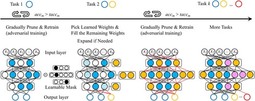
The adversarial training and continual learning procedures have been shown in Algorithm 1 and Algorithm 2, respectively, and Figure 3 illustrates the training cycle of CMAT (Algorithm 2). Moreover, Figure 4 depicts the overall operating flow of the proposed method. Here, different colours mean different tasks, and the new task weights consist of two parts: the first one selected by the learnable mask from the old task weights; and the second one learned through gradually pruning and retraining the additional weights. Because only the old task weights are selected and fixed, we can thus integrate the required function mapping with the compact model without affecting the accuracy.

Figure 3. The training cycle of the proposed approach.

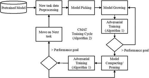
Figure 4. Operating flow of the proposed CMAT method. In the figure, x_i (i = 1∼n) represents input and different colours mean different tasks. The model is trained and retrained by calling the adversarial training algorithm (Algorithm 1). The iteration of compacting, pruning and growing is performed (Algorithm 2), in which the new task weights include those selected from the old task weights and those learned from the retraining.

Table

Algorithm 2: CMAT (compacting & prune & growing)
Input: The maximum number of task $M$, current task $m$, released weights for current task $W_m^T$, preserved weights for current task $W_m^H$, accuracy goal for every task $\mathrm{tac}{c}_m$, network with multiplier $\alpha$, max network with multiplier max_$\alpha$, prune ratio $p$, prune ratio interval $v$
Output: $\mathrm{ac}{c}_m$
1:	for  task $m=2\dots M$ (let the released weights of task $m$ be $W_m^T$) do
	# Growing phase
2:	Apply a mask $S$ to the weights $W_{1:m-1}^H$
3:	while $a$ $\le$ max_$a$ do
4:	Set an accuracy goal for task $m$
5:	Expand the number of filters (weights) of the model multiplied by $\alpha$
6:	reset $W_{m-1}^T$
7:	$\mathrm{ac}{c}_m\leftarrow \mathrm{train}\left(S,W_{m-1}^T,W_{1:m-1}^H\right)$ with Algorithm 1
8:	if $\mathrm{ac}{c}_m>\mathrm{tac}{c}_m$
9:	exit
10:	end if
11:	$a+=$0.5
12:	end while
	# Compacting & Prune phase
13:	for $i=1\dots 9$ do
14:	set prune ratio $p$
15:	Prune $W_{m-1}^T$to obtain $W_m^T$
16:	$\mathrm{ac}{c}_i\leftarrow \mathrm{train}\left(S,W_m^T,W_{1:m-1}^H\right)$ with Algorithm 1
17:	$W_m^H=W_{m-1}^T-W_m^T$ with ratio $p$
18:	$W_{1:m}^H=W_{1:m-1}^H\cup W_m^H$
19:	if $\mathrm{ac}{c}_i>\mathrm{tac}{c}_m$
20:	exit
21:	end if
22:	$p+=v$
23:	end for
24:	end for

3.3. Model compression by knowledge distillation

As indicated before, self-distillation has recently drawn much attention. This approach divides the learning model into different sections and distils the knowledge from a larger deep neural network into a small network. It allows the model to have a very flexible structure depending on the amount of available computation. Here, we develop a unified framework that integrates both multi-teacher knowledge transfer and self-distillation methods to exploit their corresponding performance fully. Our method can reduce the model size, that is, using a smaller region of the model to accommodate the knowledge learned by the teacher model with similar performance. It can be used alone to derive a lightweight image model for devices with resource limitations while providing a promising candidate to enhance the compacting effect for the continual learning approach presented above. Our distillation method regards the knowledge located in different sections as multiple teachers through corresponding to the sections of the teacher model. Then, the multi-teacher distillation technique is performed on the student model to improve its accuracy. This way, the knowledge held by each section can be fully utilised.

Our method adopts the multi-teacher model presented in (You et al., 2017) as the basis to train the student model jointly. The overall loss function includes three parts that are used to measure the loss of the student model to the data labels, the loss of the middle layers between the student and the teacher models, and the output loss between the student and the teacher models, respectively. The three types of loss for each teacher are aggregated with adaptive weights that are adjusted (learned) dynamically during the training process.

The overall approach is called Self Multiple Teacher Knowledge Distillation (SMTKD), as illustrated in Figure 5. The kernel size is 3 × 3 and the stride size is 1. Before Group 1, the input image is first convoluted into data with a dimension of 64, and after Group 1, a dimension of 256, and then 512, 1024, and 2048 after Group 2, Group 3, and Group 4, respectively. As indicated above, to generate output for loss calculation, separable convolution is performed (three times for Group 1, two times for Group 2 and one time for Group 3) to increase the dimension to 2048.

Figure 5. The overall structure and the operating flow of our distillation approach.

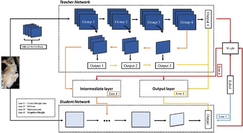
Following the approach, Loss 1 calculates the loss between the output (from the student model's SoftMax layer) and the real label, making the model learn the knowledge included in the dataset. Loss 2 measures the loss of the student and that of the teacher. Different from Loss 1, here, a hyperparameter (called Temperature) is introduced to soften the label, and a larger parameter produces a more uniform output distribution. Loss 3 is to calculate the L2 (Squared Error Loss, the squared difference between a prediction and the actual value) between the feature maps of teacher and student models. This is to introduce the ambiguous knowledge included in the feature map of the teacher into the feature map of the student. At different training stages, the student model learns knowledge from multiple teachers with different strategies to maximise the overall learning performance. Consequently, a new adaptive weight (Loss 4) is used to learn the importance of each teacher. Our method calculates cross-entropy on the output of each teacher, and then generates the weight accordingly. In addition to the external teacher model, our method also considers the situation when the student can improve gradually and eventually play the role of teacher. Here, the corresponding loss (Loss 1) is discarded, meaning that the algorithm no longer needs to set the learning rate of the teacher model, which can be changed freely during the learning process. The loss of each part is described in detail below.

3.3.1. Loss 1: cross entropy

As mentioned above, Loss 1 is to calculate the cross-entropy loss between the label and the output of the student model. This loss means to improve the student model’s predictive performance through the optimisation process. This loss function is defined in Equation (2), where NS is the SoftMax layer output of the student model, and y is the label corresponding to this dataset. (2) $\begin{array}{r}\mathrm{Loss}1=\mathrm{CrossEntropy}\left(y,N_s\right)\end{array}$(2) Training with this loss function, the student model can only learn to recognise whether the classes are correct or not. Under such circumstances, the student is not able to correctly identify similar data or data with similar classes. A scheme for softening the labels is needed to deal with such situations. Moreover, during the initial learning process, if the weight of the learning rate is too high, the student model tends to learn more information from the real labels rather than knowledge from the teacher during the learning process. In contrast, if the weight of the learning rate is too low, the student model may be biased toward the teacher model while paying no attention to the real labels.

3.3.2. Loss 2: KL (Kullback-Leibler) divergence loss under teacher’s guidance

To overcome the problem of overly relying on the real labels and ignoring the teacher’s knowledge, during the training we add a hyperparameter (Temperature) to soften the teacher label. This way, the student no longer pursues the model accuracy (Loss 1), and yet pays some attention to the similarity between different labels instead. Thus, the teacher model’s learning performance can be promoted. As indicated above, a larger parameter derives a more uniform distribution for the teacher model’s output.

The Loss 2 loss function and the Loss 1 loss function are to be balanced to exploit the corresponding advantages. In this work, we adopt the technique presented in (You et al., 2017) to achieve the balance. It is to average multiple teachers’ SoftMax layer outputs, use Temperature to soften the labels, and then perform the Temperature on the student (the student model’s SoftMax layer output). Finally, the cross-entropy is calculated. This method is called multi-teacher knowledge distillation (MTKD hereafter). This loss is defined in Equation (3) as below: (3) $\begin{array}{r}\mathrm{Loss}2=\mathrm{CrossEntropy}\left(N_{T,}^{\tau }{N}_S^{\tau }\right)\end{array}$(3) with $N_T^{\tau }=\mathrm{softmax}\left(\frac{O_T}{t}\right),N_S^{\tau }=\mathrm{softmax}\left(\frac{O_S}{t}\right)$

Here, O_T and O_S are the SoftMax model N_T and the student model $N_S$; $N_T^{\tau }$ and $N_S^{\tau }$ are the softened results of the teacher model and the student model with Temperature control.

3.3.3. Loss 3 (feature loss)

The third loss (Loss 3) is to enable the learning between the feature map of the teacher model and that of the student model. To calculate the loss, we use the FitNet algorithm presented in (Romero et al., 2015), where Loss 2 is adopted to measure the loss between the middle layers of the student and of the teacher models. This means introducing the vague knowledge in the teacher model's feature map into that of the student model.

This loss mainly considers the knowledge of the middle layer of the teacher model for learning. Although the student model can learn from the teacher model's feature map, it may not obtain the best results after going through an entire learning procedure. In fact, in the self-distillation algorithm, knowledge learning on the middle layer can obtain a good effect at the early learning stage, while overfitting may occur at the latter training stage, so the performance just declined (Luan et al., 2019). To overcome this problem, the annealing simulation method was employed to tackle this problem. Consequently, the weight of this learning part for the middle layer became high, while the weight gradually decreased during the training process.

This loss is defined in Equation (4), where $O_T^{\mathrm{inter}}$ and $O_S^{\mathrm{inter}}$ are the teacher model’s and the student model’s outputs of the middle layers. Here, r represents a linear regression with parameters ${\theta }_{\mathrm{ht}}$. (4) $\begin{array}{r}\mathrm{Loss}3=\frac{1}{2}{O}_T^{\mathrm{inter}}\left({\theta }_T\right)-r\left({\theta }_S^{\mathrm{inter}}\left({\theta }_S\right)\right);{{\theta }_{\mathrm{ht}}}_2^2\end{array}$(4)

3.3.4. Loss 4 (adaptive weight)

In a multi-teacher learning framework, different teachers’ outputs are often averaged, and the result is then provided to the student for learning. However, the importance of each teacher is, in fact, different; the smoothing effect by average thus makes both the excellent and poor teachers non-distinguishable. To overcome this problem, we present an adaptive strategy, with which the importance of each teacher is determined by performance (the output collected from the SoftMax layer) in a dynamic way. In addition to the learning effectiveness, the teacher model's learning efficiency has to be considered. That is, each teacher's convergent behaviour (learning curve) may be different from that of others. Here, the teacher's importance (weight) is assigned according to its current performance (measured at each epoch).

As mentioned above, the student model continues to benefit from multiple teachers and eventually reaches a performance level close to (or even better than) that of the teachers. In such a situation, the student can be regarded as one of the teachers. With the proposed adaptive strategy, we can take the student as a teacher with low performance initially. Through the learning procedure described above, the student model improves its performance over time, and the corresponding weight gradually increases. As the importance is measured together with the multiple teachers, a new loss (Loss 4) is defined, as shown in Equation (5): (5) $\begin{array}{r}\begin{array}{l}\mathrm{Loss}4=\mathrm{AW}=\mathrm{softmax}\left(\sum _{t=1}^m\mathrm{Max}\left(C_T\right)+\mathrm{Min}\left(C_T\right)-{\left(C_T\right)}_t\right)\\ \text{with}{C}_T=\sum _{t=1}^m\mathrm{CrossEntropy}\left(y,{\left(N_T\right)}_t\right)\end{array}\end{array}$(5)

Here m is the number of teacher models; N_T is the output of the SoftMax layer of the teacher model; y is the label corresponding to this dataset; and C_T is the result of each teacher’s cross-entropy calculation.

3.3.5. Total loss

The overall loss function is obtained by integrating the loss defined above with two hyperparameters, α and β, used to balance the different loss indicated. The final loss function is defined in equation (6)(6) $\begin{array}{r}\mathrm{Total}\mathrm{Loss}=\left(\begin{array}{c}\left(1-\alpha \right)\cdot \mathrm{Loss}1+\alpha \cdot \left(\sum _{i=1}^{m}A{W}_i\cdot \mathrm{Loss}2\left(N_{T_i}^{\tau },N_S^{\tau }\right)\right)+\\ \text{β}\cdot \left(\frac{1}{m}\sum _{i=1}^{m}A{W}_i\cdot \mathrm{Loss}3\left(O_{T_i}^{\mathrm{inter}},O_S^{\mathrm{inter}}\right)\right)\end{array}\right)\end{array}$(6) , where m is the teacher model and AW is the weight obtained by Loss 4. As indicated in Section 3.3.4, this study also considers the situation in which the student is eventually regarded as the teacher model, in which Loss 4 is used to obtain the weight to determine the role of student model. With this adaptive strategy, the knowledge distillation algorithm no longer needs to set the learning rate for the teacher model, meaning that α = 1. (6) $\begin{array}{r}\mathrm{Total}\mathrm{Loss}=\left(\begin{array}{c}\left(1-\alpha \right)\cdot \mathrm{Loss}1+\alpha \cdot \left(\sum _{i=1}^{m}A{W}_i\cdot \mathrm{Loss}2\left(N_{T_i}^{\tau },N_S^{\tau }\right)\right)+\\ \text{β}\cdot \left(\frac{1}{m}\sum _{i=1}^{m}A{W}_i\cdot \mathrm{Loss}3\left(O_{T_i}^{\mathrm{inter}},O_S^{\mathrm{inter}}\right)\right)\end{array}\right)\end{array}$(6)

4. Experiments and results

4.1. Evaluation of the proposed continual learning approach

4.1.1. Datasets and performance metrics

To evaluate the proposed approach for adversarial training, we have conducted several sets of experiments. As indicated in Section 2, our CMAT approach shared the same model with PackNet; therefore, in the first phase, we validated PackNet on various learning networks and measured the corresponding performance. The popular image dataset CIFAR-100 was used (Krizhevsky & Hinton, 2009). This dataset contained 60,000 images of 100 categories in which each image was made of 32 × 32 pixels. The dataset was initially designed and divided into training and testing subsets (each category contained 500 training images and 100 test images), and the related studies all followed the original design. In the experiments, we selected ResNet18 (He et al., 2016) and VGG16-bn (Simonyan & Zisserman, 2015) models as the representative models to examine whether or not PackNet could have a defensive effect against the adversarial examples after using PGD or FGSM for training. In these experiments, the model optimiser was Stochastic Gradient Decent (SGD), the learning rate was 0.01, and the loss function was cross-entropy. The batch size was 32 for all experiments with CIFAR-100 and 48 for others. These model parameters were chosen from the original model (Hung et al., 2019). Results were averaged over five random trials to reduce bias.

Following the related works that have regarded accuracy as the most important performance metric, our focus is also on this metric, and the results obtained with different methods can thus be compared using the same standard. Moreover, we calculated the F1 score to evaluate the proposed approach and used the macro F1 score to assess our model performance. Here, the dataset had the same number of images in each category. The metrics of accuracy and F1-macro (with precision P_macro and recall R_macro) are defined below: (7) $\begin{array}{rl}\text{accuracy}& =\frac{\text{number of correctly classified images}}{\text{number of images}}\end{array}$(7) (8) $\begin{array}{rl}\text{F}{1}_{\mathrm{macro}}& =\frac{2\times P_{\mathrm{macro}}\times R_{\mathrm{macro}}}{P_{\mathrm{macro}}+R_{\mathrm{macro}}}\end{array}$(8) (9) $\begin{array}{rl}{P}_{\mathrm{macro}}& =\frac{{\sum }_{i=1}^n{P}_i}{n}\end{array}$(9) (10) $\begin{array}{rl}{R}_{\mathrm{macro}}& =\frac{{\sum }_{i=1}^n{R}_i}{n}\end{array}$(10)

In equations (7)∼(10), P_i and R_i represent precision and recall of the classification problem i; n is the number of categories in the dataset and i refers to the n-th category.

4.1.2. Evaluation of PackNet with different attack methods

In the first set of experiments, we used CIFAR-100 dataset to evaluate the defensive effect of models by PackNet with adversarial training. The PackNet approach with adversarial examples was applied to two popular image models, ResNet18 and VGG16-bn. The better model was then chosen to work with the proposed CMAT approach in the following set of experiments.

To test the defending ability of the original model, we applied PackNet to ResNet18 (without adversarial training), and then obtained a very low accuracy of 0.076. This result indicates that without coupling adversarial training in learning, it was, in fact, difficult for the original model to provide enough defensive capability. Therefore, we modified the structure of the multiple tasks approach to include adversarial training to increase the model's ability to defend against adversarial examples. In the experiment, we applied PackNet to ResNet18 and VGG16_bn with a perturbation level 2/255 in adversarial training. We also adopted two attack methods (PGD and FGSM) to the datasets to examine the attack method that is more suitable to be used in adversarial training. Different combinations of the two attack methods were evaluated to choose the best one for later experiments.

Table 2 shows the results of our experiments. The first column indicates the attack methods used for the training and testing datasets with the step size specified. For example, PGD (7)/FGSM means that in this set of adversarial training, the PGD method was applied to the training dataset with a step size 7, and the FGSM method was applied to the testing dataset. As can be observed, the performance of using adversarial training on VGG16_bn was relatively better than that on ResNet18. The above results were consistent with the relevant studies (Madaan et al., 2020; Madry et al., 2018). Meanwhile, the effect of FGSM was not as good as that of the PGD adversarial training. Based on these results, in the following verification phase, we chose VGG16_bn network architecture with PGD adversarial training for further evaluation.

Table 2. Results of two models with different adversarial training strategies (with perturbation ϵ = 2/255).

Model	Adversarial Training	Accuracy	F1macro
ResNet18	PGD (7) / PGD (7)	0.4488	0.508
	FGSM / FGSM	0.2730	0.284
	PGD (7) / FGSM	0.2790	0.305
	FGSM / PGD (7)	0.2721	0.296
VGG16_bn	PGD (7) / PGD (7)	0.5608	0.582
	FGSM / FGSM	0.3461	0.437
	PGD (7) / FGSM	0.3626	0.407
	FGSM / PGD (7)	0.3507	0.384

To investigate the effect of perturbation in detail, we conducted two more sets of experiments on VGG16_bn with different levels of perturbation. Table 3 shows the experimental results with levels 4/255 and 8/255, respectively. Compared to the results in Table 2, the training performance in Table 3 is not as good. This indicates that the disturbance introduces training difficulty in adversarial training and the performance declined along with the increase of perturbation level (from 2/255 toward 8/255). We can also compare the effects caused by different step sizes (for PGD) from the above tables. As can be observed, the accuracy usually decreased when the step size increased. For example, with the perturbation ϵ = 2/255, the performance of using PGD slightly declined when the step size increased from 7 to 10 and then to 20. This shows that a large step size also increases task difficulty. The results in the tables show that step size 7 was the best choice for the experiments here, so it was used in the following evaluation trials.

Table 3. VGG16_bn with different levels of perturbation and different step sizes.

$ϵ$	Adversarial Training	Accuracy	F1macro
4/255	PGD (7) / PGD (7)	0.4772	0.587
	PGD (10) / PGD (10)	0.4617	0.561
	PGD (20) / PGD (20)	0.4425	0.487
8/255	PGD (7) / PGD (7)	0.4482	0.542
	PGD (10) / PGD (10)	0.4234	0.532
	PGD (20) / PGD (20)	0.3653	0.457

4.1.3. Evaluation of CMAT

In the second phase, we conducted another set of experiments to evaluate the proposed CMAT method. The parameters and the experimental settings were the same as those used for PackNet evaluations. This series of experiments was designed to verify the effectiveness of continual learning (with the operations of its pruning and growing phases) for CMAT. The results are presented in Table 4. As shown, when the setting of PGD (7) with ϵ = 2/255 was used for both training and testing datasets, the best performance could be obtained, and the results were consistent with those for PackNet in Tables 2 and 3. Overall, the model accuracy of using CMAT was about 3∼4%, higher than the results gained from using PackNet. As can be observed, the F1-score obtained from using CMAT was also better than from PackNet.

Table 4. Results of the proposed approach with different training strategies and different levels of perturbation.

$ϵ$	Adversarial Training	Accuracy	F1macro
2/255	PGD (7) / PGD (7)	0.6153	0.710
	PGD (10) / PGD (10)	0.5445	0.667
	PGD (20) / PGD (20)	0.5198	0.645
4/255	PGD (7) / PGD (7)	0.5130	0.665
	PGD (10) / PGD (10)	0.4548	0.616
	PGD (20) / PGD (20)	0.4319	0.539
8/255	PGD (7) / PGD (7)	0.4722	0.571
	PGD (10) / PGD (10)	0.4381	0.554
	PGD (20) / PGD (20)	0.4263	0.487

After evaluating the effects by using PackNet and CMAT under various conditions, we compared the performance of our CMAT approach with other methods presented in relevant studies. These methods include Adversarial Training (the primary adversarial trained network) (Madry et al., 2018), Free Adversarial Training (improved adversarial training) (Madry et al., 2018), Pretrained Adversarial Training (adversarial training with pre-trained weights) (Hendrycks et al., 2019), TRADES (adversarial training with a theoretically principled trade-off between robustness and accuracy) (Zhang et al., 2019b), and ANP-VS (adversarial training that combines pruning and vulnerability suppression loss) (Madaan et al., 2020). In the experiments, the dataset CIFAR-100 was used, and the parameters for PGD adversarial training of the original works included the perturbation level ϵ = 8/255, the training step size 10, and the testing step size 40. The results of different approaches are given in Table 5, in which our results are in contrast with those of other methods addressed in (Madaan et al., 2020).

Table 5. Results of different training approaches.

Method	Accuracy
Adversarial training (Madry et al., 2018)	0.3247
Free adversarial training (Madry et al., 2018)	0.3038
Pretrained adversarial training (Hendrycks et al., 2019)	0.3542
TRADES (Zhang et al., 2019b)	0.3281
ANP-VS (Madaan et al., 2020)	0.3701
PackNet (Madaan et al., 2020)	0.4113
CMAT (the proposed approach)	0.4591

In the experiments by PackNet and CMAT, we adopted the same parameter settings to keep the comparison on the same standard. As shown in Table 5, the results of PackNet and CMAT are obviously better than others. Compared to other methods, PackNet outperformed the primary adversarial training method by 0.087 (accuracy), and the most similar method ANP-VS by 0.041; and CMAT was even better than PackNet by 0.048. These results prove that the proposed approach is capable of defending adversarial examples and related attacks to gain better performance. All confirm the effectiveness and transferability of the proposed approach.

In the third phase, we conducted experiments on additional image datasets to investigate whether our GMAT approach was able to defend adversarial examples in situations closer to real-life scenarios. The best settings have been chosen from the previous experiments for this set of experiments, and trained the VGG16_bn model with both PackNet and our GMAT approach on four datasets (CUBS, Stanford Cars, Flowers, and Sketches) for performance comparison. Table 6 is the summary of the four datasets. Different from other image datasets, the last dataset (Sketches) contains non-expert sketches of everyday objects, initially created for sketch recognition.

Table 6. Summary of the high-resolution datasets.

Dataset	Train	Val.	Category
CUBS	5994	5794	200
Standard Cars	8144	5794	196
Flowers	2040	6149	102
Sketches	16000	4000	250

Table 7 presents the results. As shown, the proposed approach is better than PackNet in two different adversarial training strategies. These results are consistent with those obtained in the previous experiments. All confirm the effectiveness of the proposed approach. For the Sketches dataset, both our CMAT approach and PackNet obtained deficient performance. Nevertheless, the accuracy of our approach is still better. The reason for the low performance could be that the categories of the black-stroke sketches were initially difficult to correctly recognise, and the perturbation worsened the situation and performance. More effective solutions for this special type of datasets are required.

Table 7. Results of different training settings.

Method	Training Strategy	CUBS	Cars	Flowers	Sketches
PackNet	PGD (7) / PGD (7)	0.5346	0.7693	0.6945	0.1147
	PGD (10) / PGD (10)	0.4964	0.7317	0.6713	0.1013
CMAT	PGD (7) / PGD (7)	0.5689	0.7892	0.7456	0.1214
	PGD (10) / PGD (10)	0.5361	0.7549	0.7031	0.1071

4.2. Evaluation of proposed knowledge distillation approach

4.2.1. Datasets and performance metric

In this work, several sets of experiments have been conducted to evaluate the proposed approach of multi-teacher with knowledge distillation. In the experiments, the CIFAR-100 dataset was used. Following the relevant studies in knowledge distillation that used accuracy as the performance metric, we also adopted it to evaluate the proposed approach. As in the experiments described in the above section, five random trials were performed, and the average results were presented.

4.2.2. Teacher training with knowledge distillation

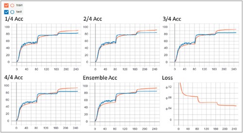
In our experiments, the ResNet50 model was adopted as the student model and a larger model, ResNet152, was used as the teacher model. To ensure the performance of the teacher model (ResNet152), in the first phase, we conducted a set of trials to evaluate this model using the self-distillation technique. As mentioned in Section 3.3, the model (ResNet152) was divided into four shallow sections according to their depth (ResBlocks), and additional bottleneck and fully connected layers were set for each section, which constitutes multiple classifiers (namely 1/4, 2/4, 3/4, 4/4 hereafter), with an additional ensemble output (to be a classifier) as reported in the original work (Zhang et al., 2019a). All classifiers can be utilised independently, with different accuracy and response time.

In this set of experiments for teacher training, the batch size was 128, the optimisation method was SGD, the learning rate was 0.1, and each trial was performed for 250 epochs. The results are presented in Figure 6, in which the accuracy for each classifier and the training loss are depicted. The best model was obtained at epoch 225, with an accuracy of 85.79 (%). The results (accuracy) for the classifiers are 82.44% (1/4), 84.60% (2/4), 84.43% (3/4) and 83.93% (4/4) respectively. These results verify that this model can be trained with good performance by the self-distillation technique and can work as the teacher to transfer knowledge to the student model.

Figure 6. Performance of training ResNet152 SD with dataset CIFAR 100.

4.2.3. Evaluation of different multi-teacher methods with self distillation

After examining the performance of the teacher model, in the second phase, we adopted this model to perform knowledge transfer from teacher to student with three multi-teacher strategies to evaluate the proposed approach. The goal here is to assess the performance of transferring knowledge from pretrained teacher models to a small student model (a lightweight model) by training with a small amount of data. We thus randomly sampled 20% of the amount of data from the CIFAR-100 dataset to train the student model.

The strategies include MTKD, SMTKD and SMTKDS (SMTKD with the student as one of the teachers). For all three methods, the experimental setup was the same as described in the previous section. For the baseline model MTKD, the multiple teachers represented the divided sections, and their outputs (knowledge) were averaged as the overall result (You et al., 2017). For the second method, SMTKD, additional parameter configuration was needed: Temperature was 2, the loss weights α was 0.9 and β was 0.3 in the total loss Equation (6). These parameters were chosen based on a preliminary test, with details listed in Table 8.

Table 8. Results of different combinations for parameters α and β.

α	β	Accuracy
0.5	0.03	68.11
0.5	0.1	66.14
0.5	0.3	66.91
0.7	0.03	68.92
0.7	0.1	68.57
0.7	0.3	68.44
0.9	0.03	70.08
0.9	0.1	69.56
0.9	0.3	70.16

A series of experiments was conducted to investigate the performance of the three multi-teacher methods mentioned and the effect of different numbers of teachers used in the distillation process. Five sets of trials were performed for each method, including using one classifier (ensemble or the deepest classifier) and multiple classifiers (with 2, 3, 4, or 5 classifiers) as teachers. Table 9 lists the results, showing the accuracy of each classifier in detail, and Figure 7 also illustrates the results. The loss converging behaviour of all three multi-teaches was the same as the loss curve shown in Figure 6. The results demonstrate that all three methods have obtained better results, and among them, the proposed approach performed the best. To sum up, more teachers used in the distillation process can obtain higher performance. The effect is especially obvious for the proposed approach, in which the best result (71.33%) is obtained with five teachers by the proposed SMTKDS method.

Figure 7. Performance of three methods with different numbers of teachers.

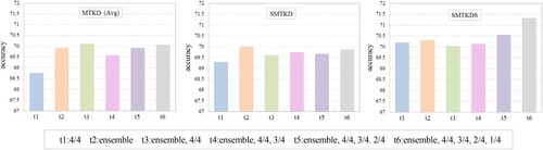
Table 9. Performance comparison of three multi-teacher knowledge distillation methods.

Method	num. of teacher (teachers)	4/4	3/4	2/4	1/4	Ensemble
MTKD (Avg.)	1 (4/4)	66.72	65.78	66.94	65.78	68.76
	1 (Ensemble)	68.83	66.47	67.96	66.29	69.92
	2 (Ensemble, 4/4)	68.72	66.91	67.92	67.17	70.12
	3 (Ensemble, 4/4, 3/4)	68.07	66.07	67.86	66.12	69.59
	4 (Ensemble, 4/4, 3/4, 2/4)	68.73	66.42	68.03	66.61	69.92
	5 (Ensemble, 4/4, 3/4, 2/4, 1/4)	68.38	65.69	68.60	66.71	70.06
SMTKD	1 (4/4)	67.83	66.20	67.13	65.85	69.29
	1 (Ensemble)	68.58	66.31	68.36	67.03	70.01
	2 (Ensemble, 4/4)	68.28	66.53	68.10	66.60	69.61
	3 (Ensemble, 4/4, 3/4)	67.92	66.19	67.91	66.76	69.75
	4 (Ensemble, 4/4, 3/4, 2/4)	68.59	65.86	67.59	66.40	69.67
	5 (Ensemble, 4/4, 3/4, 2/4, 1/4)	68.31	65.89	67.72	66.53	69.87
SMTKDS (ours)	1 (4/4)	68.05	66.50	68.92	66.93	70.20
	1 (Ensemble)	69.00	66.80	68.81	67.34	70.31
	2 (Ensemble, 4/4)	68.70	66.48	68.29	66.88	70.04
	3 (Ensemble, 4/4, 3/4)	68.58	66.35	68.42	67.18	70.14
	4 (Ensemble, 4/4, 3/4, 2/4)	69.36	66.59	68.34	66.96	70.55
	5 (Ensemble, 4/4, 3/4, 2/4, 1/4)	70.14	67.51	69.46	67.97	71.33

4.2.4. Evaluation of knowledge transfer with different amount of data

In addition to evaluating the performance of the number of teachers used, we also conducted experiments to investigate the effect of various data amounts used in student training by multi-teacher knowledge distillation methods. For each multi-teacher method, five trials were performed, using 20%, 40%, 60%, 80%, and 100% data. The results are listed in Table 10, including the original student model without a teacher. Similar to the general cases of model training, more training data can obtain better performance for all three methods, and a larger improvement made by the teachers can be observed for a small amount of data in training (e.g. 20%). To sum up, among the three multi-teacher methods, the proposed approach can obtain the best performance for the cases using a small amount of data.

Table 10. Performance comparison of three multi-teacher knowledge distillation methods with different amount of training data.

	data amount
Method	20%	40%	60%	80%	100%
Original	65.98	75.20	80.37	83.04	85.07
MTKD (Avg)	70.06	79.54	82.76	84.69	85.75
SMTKD	69.87	79.43	82.55	84.83	85.38
SMTKDS (ours)	71.33	79.81	82.85	84.65	85.73

5. Conclusion

In this work, we investigate the critical issues regarding adopting deep learning methods to train secured image recognition models for vision-based systems. We develop a framework to address two crucial issues that lightweight devices often suffer. The first issue is about training robust defensive models through iteratively generating adversarial examples and then including these examples in the learning procedure. To achieve this goal, we design a new adversarial training approach that integrates continual learning and progressive adversarial training for robustness enhancement. Our approach includes dynamic phases of growing and compacting a model in the process of continual learning. It performs adversarial training that aggregates, augments and injects adversarial noises progressively. In this way, the trained recognition model can be robust against attacks because it has an adaptive structure to learn new tasks sequentially. The second issue is about training a lightweight model suitable for working with other special learning approaches or for the deployment of mobile devices. We develop a new knowledge distillation approach to integrate both self-distillation and multi-teacher distillation techniques. Our approach has a specially designed student-teacher learning structure with a new loss function, enabling the small student model to distil knowledge from a large pretrained teacher model and at the same time to keep performance close to the teacher model. To evaluate the performance of the proposed approach, we conduct a series of experiments to compare it with other methods. For adversarial training, the model accuracy by using our CMAT was higher than that by PackNet in cases with different levels of perturbation. CMAT also outperformed other approaches in further comparison under the same experimental settings. The results show that our approach can obtain the best performance. As for the lightweight modelling, the results reveal that more teachers can result in higher performance and the effect is pronounced for the proposed SMTKDS approach towards obtaining the best result. In the experiments of training the student model with a small amount of data, SMTKDS can best improve the student model. These results verify that a small model can be trained through the proposed approach; it is indeed a practical and valuable method.

As for the limitations of the proposed approach, in the experimental implementation, the training time of the adversarial training increased along with the task difficulty (i.e. the increases of disturbance or step size), though more robust models can be obtained. Similarly, the self-distillation of the student model can improve the overall performance while more training time is required. There is a tradeoff between performance and computational cost. At present, more and more advanced techniques have been undertaken to reduce the computational cost. Also, limited by the characteristics of the datasets, the improvement varies from dataset to dataset. Enhanced schemes can be developed further. Based on the presented work, we are currently exploring the effectiveness of adversarial examples and developing an adaptive student-teacher network for knowledge distillation. We are also developing adaptive strategies to determine the relevant parameters of the proposed approach automatically. Moreover, we plan to build new mechanisms to integrate the approaches of adversarial training and knowledge distillation to obtain more comprehensive models for performance improvement.

Declarations

Availability of supporting data

The data used in this work is publicly accessible and has been identified in the text.

Authors’ contributions

T.C.: Software, Methodology; Y.K.: Data curation, Software; J.H.: Validation, Writing – review & editing; W.L.: Conceptualization, Methodology, Investigation, Supervision, Writing – original draft.

Disclosure statement

No potential conflict of interest was reported by the author(s).

Additional information

Funding

This research was supported in part by National Science and Technology Council of Taiwan, under Contract NSTC-112-2221-E-110-054.

References

- Aldahdooh, A., Hamidouche, W., Fezza, S. A., & Déforges, O. (2022). Adversarial example detection for DNN models: A review and experimental comparison. Artificial Intelligence Review, 55, 4403–4462. https://doi.org/10.1007/s10462-021-10125-w
- Cai, Q. Z., Du, M., Liu, C., & Song, D. (2018). Curriculum adversarial training. arXiv preprint arXiv:1805.04807v1.
- Chou, T.-C., Huang, J.-Y., & Lee, W.-P. (2022). Continual learning with adversarial training to enhance robustness of image recognition models. Proceedings of the 21st International Conference on Cyberworlds, 236–242.
- Cossu, A., Carta, A., Lomonaco, V., & Bacciu, D. (2021). Continual learning for recurrent neural networks: An empirical evaluation. Neural Networks, 143, 607–627. https://doi.org/10.1016/j.neunet.2021.07.021
- Croce, F., & Hein, M. (2020). Reliable evaluation of adversarial robustness with an ensemble of diverse parameter-free attacks. Proceedings of the 37th International Conference on Machine Learning, 2206–2216.
- Crowley, E. J., Gray, G., & Storkey, A. J. (2018). Moonshine: Distilling with cheap convolutions. Proceedings of the 32nd International Conference on Neural Information Processing Systems, 2893–2903.
- Du, F., Yang, Y., Zhao, Z., & Zeng, Z. (2023). Efficient perturbation inference and expandable network for continual learning. Neural Networks, 159, 97–106. https://doi.org/10.1016/j.neunet.2022.10.030
- Furlanello, T., Lipton, Z., Tschannen, M., Itti, L., & Anandkumar, A. (2018). Born again neural networks. Proceedings of the 35th International Conference on Machine Learning, 1607–1616.
- Gao, M. (2023). A survey on recent teacher-student learning studies. Journal of the ACM, 37, article 111.
- Gao, M., Wang, Y., & Wan, L. (2021). Residual error-based knowledge distillation. Neurocomputing, 433, 154–161. https://doi.org/10.1016/j.neucom.2020.10.113
- Goodfellow, I., Shlens, J., & Szegedy, C. (2015). Explaining and harnessing adversarial examples. Proceedings of the 3rd International Conference on Learning Representation.
- Gou, J., Yu, B., Maybank, S. J., & Tao, D. (2021). Knowledge distillation: A survey. International Journal of Computer Vision, 129, 1789–1819. https://doi.org/10.1007/s11263-021-01453-z
- Guo, Y., Liu, B., & Zhao, D. (2023). Dealing with cross-task class discrimination in online continual learning. Proceedings of the IEEE/CVF Conference on Computer Vision and Pattern Recognition, 11878–11887.
- Han, S., Lin, Y., Guo, Z., & Lv, K. (2023). A lightweight and stylerobust neural network for autonomous driving in end side devices. Connection Science, 35, 2155613. https://doi.org/10.1080/09540091.2022.2155613
- He, K., Zhang, X., Ren, S., & Sun, J. (2016). Deep residual learning for image recognition. Proceedings of IEEE Conference on Computer Vision and Pattern Recognition, 770–778.
- Hendrycks, D., Lee, K., & Mazeika, M. (2019). Using pre-training can improve model robustness and uncertainty. Proceedings of the 36th International Conference on Machine Learning, 2712–2721.
- Hinton, G. E., & Salakhutdinov, R. R. (2006). Reducing the dimensionality of data with neural networks. Science, 313, 504–507. https://doi.org/10.1126/science.1127647
- Hinton, G., Vinyals, O., & Dean, J. (2015). Distilling the knowledge in a neural network. arXiv preprint arXiv:1503.02531v1.
- Hung, C. Y., Tu, C.-H., Wu, C.-E., Chen, C.-H., Chan, Y.-M., & Chen, C.-S. (2019). Compacting, picking and growing for unforgetting continual learning. Proceedings of the 30th International Conference on Neural Information Processing Systems, 13647–13657.
- Incel, O. D., & Bursa, SÖ. (2023). On-device deep learning for mobile and wearable sensing applications: A review. IEEE Sensors Journal, 23, 5501–5512. https://doi.org/10.1109/JSEN.2023.3240854
- Joseph, K. J., Khan, S., Khan, F. S., & Balasubramanian, V. N. (2021). Towards open world object detection. Proceedings of IEEE/CVF Conference on Computer Vision and Pattern Recognition, 5830–5840.
- Krizhevsky, A., & Hinton, G. (2009). Learning multiple layers of features from tiny images. Technical Report TR-2009. University of Toronto.
- Kurakin, A., Goodfellow, I., & Bengio, S. (2017). Adversarial examples in the physical world. Proceedings of the 5th International Conference on Learning Representation Workshop Track.
- Liu, A., Liu, X., Yu, H., Zhang, C., Liu, Q., & Tao, D. (2021). Training robust deep neural networks via adversarial noise propagation. IEEE Transactions on Image Processing, 30, 5769–5781. https://doi.org/10.1109/TIP.2021.3082317
- Luan, Y., Zhao, H., Yang, Z., & Dai, Y. (2019). MSD: Multi-self-distillation learning via multi-classifiers within deep neural networks. arXiv preprint arXiv:1911.09418v3.
- Ma, L., & Liang, L. (2022). Increasing-margin adversarial (IMA) training to improve adversarial robustness of neural networks. arXiv preprint arXiv:2005.09147v10.
- Madaan, D., Shin, J., & Hwang, S. J. (2020). Adversarial neural pruning with latent vulnerability suppression. Proceedings of the 37th International Conference on Machine Learning, 6531–6541.
- Madry, A., Makelov, A., Schmidt, L., Tsipras, D., & Vladu, A. (2018). Towards deep learning models resistant to adversarial attacks. Proceedings of the 6th International Conference on Learning Representation.
- Mallya, A., & Lazebnik, S. (2018). Packnet: Adding multiple tasks to a single network by iterative pruning. Proceedings of IEEE Conference on Computer Vision and Pattern Recognition, 7765–7773.
- Mirzadeh, S. I., Farajtabar, M., Li, A., & Ghasemzadeh, H. (2020). Improved knowledge distillation via teacher assistant. Proceedings of the 34th AAAI Conference on Artificial Intelligence, 5191–5198. https://doi.org/10.1609/aaai.v34i04.5963
- Mundt, M., Hong, Y., Pliushch, I., & Ramesh, V. (2023). A wholistic view of continual learning with deep neural networks: Forgotten lessons and the bridge to active and open world learning. Neural Networks, 160, 306–336. https://doi.org/10.1016/j.neunet.2023.01.014
- Nowak, T. S., & Corso, J. J. (2018). Deep net triage: Analyzing the importance of network layers via structural compression. arXiv preprint arXiv:1801.04651v2.
- Pfülb, B., & Gepperth, A. (2019). A comprehensive, application-oriented study of catastrophic forgetting in DNNs. Proceedings of the 7th International Conference on Learning Representation.
- Rice, L., Wong, E., & Kolter, J. Z. (2020). Overfitting in adversarially robust deep learning. Proceedings of the 37th International Conference on Machine Learning, 8093–8104.
- Romero, A., Ballas, N., Kahou, S. E., Chassang, A., Gatta, C., & Bengio, Y. (2015). Fitnets: Hints for thin deep nets. Proceedings of the 3rd International Conference on Learning Representation.
- Rusu, A. A., Rabinowitz, N. C., Desjardins, G., Soyer, H., Kirkpatrick, J., Kavukcuoglu, K., Pascanu, R., & Hadsell, R. (2016). Progressive neural networks. arXiv preprint arXiv:1606.04671v3.
- Schwarz, J., Luketina, J., Czarnecki, W. M., Grabska-Barwinska, A., Teh, Y. W., Pascanu, R., & Hadsell, R. (2018). Progress & compress: A scalable framework for continual learning. Proceedings of the 35th International Conference on Machine Learning, 4535–4544.
- Simonyan, K., & Zisserman, A. (2015). Very deep convolutional networks for large-scale image recognition. Proceedings of the 3rd International Conference on Learning Representations.
- Song, H., Kim, M., Park, D., Shin, Y., & Lee, J.-G. (2023). Learning from noisy labels with deep neural networks: A survey. IEEE Trans. on Neural Networks and Learning Systems, 34, 8135–8153. https://doi.org/10.1109/TNNLS.2022.3152527
- Szegedy, C., Zaremba, W., Sutskever, I., Bruna, J., Erhan, D., Goodfellow, I., & Fergus, R. (2014). Intriguing properties of neural networks. Proceedings of the 2nd International Conference on Learning Representation.
- Tramèr, F., Kurakin, A., Papernot, N., Goodfellow, I., Boneh, D., & McDaniel, P. (2018). Ensemble adversarial training: Attacks and defenses. Proceedings of the 6th International Conference on Learning Representations.
- Wang, H., Zhao, H., Li, X., & Tan, X. (2018). Progressive blockwise knowledge distillation for neural network acceleration. Proceedings of the 27th International Joint Conference on Artificial Intelligence, 2769–2775.
- You, S., Yu, C., Xu, C., & Tao, D. (2017). Learning from multiple teacher networks. Proceedings of the 23rd ACM SIGKDD International Conference on Knowledge Discovery and Data Mining, 1285–1294.
- Yu, H., Liu, A., Li, G., Yang, J., & Zhang, C. (2021). Progressive diversified augmentation for general robustness of DNNs: A unified approach. IEEE Trans. on Image Processing, 30, 8955–8967. https://doi.org/10.1109/TIP.2021.3121150
- Yuan, X., He, P., Zhu, Q., & Li, X. (2019). Adversarial examples: Attacks and defenses for deep learning. IEEE Trans. on Neural Networks and Learning Systems, 30, 2805–2824. https://doi.org/10.1109/TNNLS.2018.2886017
- Zhang, L., Song, J., Gao, A., Chen, J., Bao, C., & Ma, K. (2019a). Be your own teacher: Improve the performance of convolutional neural networks via self-distillation. Proceedings of IEEE/CVF International Conference on Computer Vision, 3713–3722.
- Zhang, J., Xu, X., Han, B., Niu, G., Cui, L., Sugiyama, M., & Kankanhalli, M. (2020). Attacks which do not kill training make adversarial learning stronger. Proceedings of the 37th International Conference on Machine Learning, 11278–11287.
- Zhang, H., Yu, Y., Jiao, J., Xing, E. P., Ghaoui, L. E., & Jordan, M. I. (2019b). Theoretically principled trade-off between robustness and accuracy. Proceedings of the 36th International Conference on Machine Learning, 7472–7482.
- Zhu, M., & Gupta, S. (2018). To prune, or not to prune: Exploring the efficacy of pruning for model compression. Proceedings of International Conference on Learning Representation Workshop Track.