New evidence on using expert ratings to proxy for wine quality in climate change research

ABSTRACT

This paper provides new evidence on the validity of using expert ratings of wine as a measure of wine quality for predicting the effects of climate change on the wine industry. We used Bob Campbell’s ratings of New Zealand wines to look for a relationship between the ratings and climatic variables that predicts a plausible optimal growing-season temperature for the main wine varieties and wine regions in New Zealand. Such a relationship can be used to forecast the effects of climate change on wine quality to better understand when wineries need to adapt to a warming climate. We used both individual wine ratings and overall vintage ratings, averaged by region and variety from the individual ratings, to compare in a controlled setting their success in predicting plausible optimal temperatures. We find that using the vintage ratings produces substantially more precise and plausible findings than using the individual ratings. We conclude that there is great potential in using vintage data constructed from expert ratings for individual wines for climate change research.

KEYWORDS:

• Weather
• climate change
• wine score
• expert rating
• wine quality

1. Introduction

It is an undeniable fact that wine regions around the world are being affected by climate change.¹ This is important because the quality of fine wine depends on the quality of the grapes, which itself is affected by the climatic conditions during the wine-growing season (See for example Ashenfelter & Storchmann, 2016; Blanco-Ward et al., 2019; Hannah et al., 2013; Mozell & Thach, 2014; Tate, 2001; and Corte-Real et al., 2015, 2017). Climate change has increased the average global temperature by more than one degree Celsius since 1880, and this warming trend is picking up pace (Turner et al., 2009). Higher temperatures lead to grapes ripening earlier in the growing season, which affects the composition of the grapes and ultimately impacts the quality of the wine (Blanco-Ward et al., 2019; van Leeuwen & Darriet, 2016). Regions that traditionally focused on cool-climate varieties and styles, the quality of which often suffers from insufficient ripening before harvest, may benefit from some warming of their climates. However, excessive warming may force winemakers to consider varieties that are more suited to warmer climates. Regions that are already producing warm-climate varieties will, eventually, no longer be able to produce the quality the region has been accustomed to (Ashenfelter & Storchmann, 2016).

When trying to understand how climate change affects the quality of wine, we need to know the empirical relationship that associates the quality of a wine to weather variables. Such a relationship can then be used to predict future wine quality in the face of climate change. There is a lively discussion in the wine economics literature on whether it is legitimate to use the ratings of wine critics as a reliable measure of the quality of wine. Concerns arise due to the potential for subjectivity of ratings across critics. Studies have found that weather alone can be a better predictor of the quality of a wine than a wine critic (see for example Haeger & Storchmann, 2006 and Ashenfelter & Jones, 2013). However, because the goal of our research is to understand how the changes in the climatic variables affect the quality of a variety, we need a measure of quality that is distinct from weather. Two available options are using wine prices and using wine ratings (see Section 2 for a detailed discussion on these), but because reliable price data is not available for New Zealand wines, we use wine ratings in our research.

This paper has two goals. First, in light of criticism of the method, we want to provide further evidence of the plausibility of using expert ratings as a measure of wine quality in climate change research. Among those in the literature that use expert wine ratings to predict the effects of climate change on viticulture, Jones et al. (2005) use vintage ratings of a wine region (single annual observation) as the explanatory factor, while Ramirez (2008) and Oczkowski (2016) use ratings of individual wines. Our innovation is to use both ratings of individual wines and regional variety-specific vintage scores, created by averaging the individual ratings, and to compare the two methods’ ability to generate plausible results in a controlled setting. The second goal of this research is to better understand how climate change impacts the quality of different wine varietals within the wine regions in New Zealand. By doing so, we start to understand how climate change might drive the need for the wine industry to adapt away from growing traditional varieties in some regions.

In this study we use Bob Campbell's wine ratings as measures of wine quality. Bob Campbell is one of the most respected wine experts in New Zealand and has, by far, the most extensive dataset of rated New Zealand wines. We use a number of regression models and techniques to estimate a relationship between the rating of a wine and a set of mostly climatic control variables. Our focus is on understanding the effect of the growing-season average temperature on the wine rating, which in turn allows us to predict the optimal temperature for each variety. The predicted optimal temperature can be compared with the current temperature and the forecasted future temperatures to understand the need for the wine regions to adapt to climate change.

Studies that focus on predicting the value of a mature wine using weather data tend to use a linear model of the growing-season temperature. However, we need to use a quadratic model to be able to use the results to predict the long-term effects of climate change, understanding that for each grape varietal there will be a threshold temperature beyond which further increases in the growing-season temperature will reduce the quality of the wine. For us to be able to confidently use our results to predict the effects of climate change on the industry, it is essential that we find a positive coefficient for the linear temperature term and a negative coefficient for the quadratic term. These results together imply that there is a temperature optimum beyond which further increases in temperature reduce wine quality. Furthermore, the optimal temperature point estimates, derived from our coefficient estimates, need to be in line with findings from other countries for the grape varieties that we investigate, although some variation can be expected due to differences in regional wine-making styles.

Our overall finding is that the results are substantially more precise and plausible when we use the constructed vintage data than when we use the original individual wine-level data. Thus, it seems that the process of averaging the scores for each region and year removes some ‘noise’ that makes it difficult to identify the underlying relationship between the quality of wine and weather. Averaging across regions and years would certainly dampen the impact of any subjective bias in the ratings across individual wines. We conclude that there is great potential in the use of vintage data – either readily available data or constructed data as in our study – to understand the long-term prospects of wine varieties in a given region.

The remainder of the paper is organised as follows. Section 2 discusses the different measures of wine quality used in previous research. Section 3 presents a brief description of the New Zealand wine regions. Section 4 describes the data sources and variables used in the regression analysis and Section 5 presents the methodology and models. Section 6 presents summary statistics of our data, and the main results are presented and discussed in Section 7. Section 8 concludes.

2. Measures of wine quality

In this section, we discuss three ways to measure wine quality that are commonly used in the literature. The first approach uses the price, preferably an auction price that varies from vintage to vintage, to measure quality. The second approach uses vintage scores, published by wine experts, to measure the quality of a vintage of a particular variety. The third approach uses wine critics’ ratings of individual wines to measure quality.

2.1. Auction price as a measure of quality

In pioneering work in the field, Ashenfelter identified predictors of auction prices of a small number of Bordeaux Chateaux wines. Known as the ‘Bordeaux equation’, Ashenfelter’s model attributes higher wine quality, as measured by mature-wine auction prices, to higher growing-season temperature, higher dormant-season rainfall and lower harvest rainfall. It has been successful in predicting prices of mature wines, often surpassing the predictive power of the expert wine tasters who, at time of harvest, predicted the future quality of a wine at maturity (Ashenfelter, 2008, 2010; Ashenfelter et al., 1995). Byron and Ashenfelter (1995) used the same equation to successfully predict mature-wine auction prices of a single Australian wine, Penfold’s Grange Hermitage. Wood and Anderson (2006) used Langton’s auction data for three iconic Australian red wines.

In theory, prices are more likely to reflect the quality of the wine in a given vintage when prices vary upwards and downwards from vintage to vintage and when consumer information is reflected in the prices. These conditions are met with fine mature-wine auctions where fluctuations in vintage quality lead to fluctuations in demand that immediately affect price levels. Ashenfelter (2008, 2010) found that the auction price of a vintage of a given wine by the same winemaker and from the same block can vary by a factor of 20 depending on the quality of that vintage. Where mature-wine auctions are not commonplace, using retail prices could be an option. However, they tend not to vary from vintage to vintage, especially not downwards, making them problematic for using as the measure of quality in climate change research. Having said that, Haeger and Storchmann (2006) successfully used the recommended retail prices of 451 California and Oregon Pinot Noir rated in the Wine Spectator in 1998–2003 and found that the relationship between a price and the growing-season temperature is a positive, concave function.

2.2. Experts’ vintage rating as a measure of quality

An alternative way to measure the quality of the wine is to use experts’ ratings. While the average wine consumer relies on expert opinion (Storchmann, 2012), the ability and integrity of wine critics have been questioned by many researchers (see for example Goldstein, 2008; Hodgson, 2008; and Reuter, 2009). Regardless, expert opinion is often the best or even only available information about wine quality at time of purchase for consumers. Ashenfelter and Jones (2013) found that experts’ ratings add some predictive power to regressions that estimate auction prices as functions of weather variables, potentially justifying the use of experts’ ratings to measure quality when no data on auction prices exists.

Most research using experts’ ratings to understand the effect of climate change uses vintage ratings rather than rating of individual wines. Vintage ratings are favoured because there is often more agreement about them than about ratings of individual wines. Also, using vintage scores avoids the complications that arise when variations in winemaking affect wine quality. Jones et al. (2005) used the Sotheby's vintage ratings to study the effect climate has on wine quality for the dominant varieties grown in important wine regions around the world. They found a significant, concave relationship between growing-season temperature and vintage rating for some varieties and regions while for others the relationship was found to be either insignificant or convex. The results of Jones et al. suggest that wine regions in Europe are currently experiencing optimal growing season temperatures for the grapes traditionally grown in those regions. They also suggest that, by 2050, the wine quality in Europe may well start to decline unless wineries are able to adapt to climate change by growing new varieties or adopting new wine-making techniques and wine styles. However, their findings suggest that the relationship is less clear for the New World wine regions. Other research using vintage ratings includes Grifoni et al. (2006) and Corsi and Ashenfelter (2019), both of which studied the effect of weather on a selection of prestigious North-Western Italian wines. While Grifoni et al. found that higher vintage scores were associated with higher temperatures and lower rainfall during the growing season, Corsi and Ashenfelter found weak results at best, with only summer rain having a significant coefficient with the predicted sign. Baciocco et al. (2014) used consensus ranking of vintages to study the effect of weather on Bordeaux red and sweet white wine vintage rankings. They found ratings to increase with growing season temperature and decrease with growing season rain for both wine types. Sadras et al. (2007) used the vintage ratings of 24 Australian wine regions over 25 years and found that an increase in the average temperature has had a positive effect on the ratings of red vintages and reduced the ratings’ variability from year to year, but these results were not found for the vintages of white wines. Jones and Davis (2000) used Bordeaux vintage ratings to study the two main red Bordeaux varieties – Merlot and Cabernet Sauvignon – and found that the variations in vintage quality were mostly derived from the variation in the characteristics of Cabernet Sauvignon.

2.3. Experts’ rating of individual wines as a measure of quality

A small number of papers use experts’ ratings of individual wines to proxy the quality of wines. Ramirez (2008) used Wine Spectator scores of all Napa Valley Cabernet Sauvignon to study the effect of weather on ratings and prices. He found that, while roughly 70% of the variation in prices could be explained by weather, only about 3% of the variation in expert ratings was explained by weather. He also found that many of the coefficients’ signs in the rating regressions were either inconsistent with expectations or not statistically significant. Most importantly, he did not find a positive effect for the two temperature variables in his model that cover the growing season. Oczkowski (2016) used ratings from Halliday (2014) to study the weather-rating and the rating-price relationships for a number of Australian varieties. He found the expected concave relationship for the growing-season temperature to be significant for Cabernet Sauvignon, Chardonnay, Merlot, Pinot Noir, Sauvignon Blanc and Shiraz while the effect was found to be convex for Riesling and Semillon. He also found a consistent and negative effect of harvest rainfall.

3. Study area

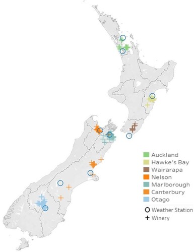
There are seven main wine regions in New Zealand, ranging geographically from Auckland in the north of the North Island to Otago in the southern part of the South Island. Figure 1 illustrates these regions as clusters of the wineries in our database. It also shows the National Institute of Water and Atmospheric Research [NIWA] weather stations that were matched to the study’s wineries. As the wine regions are quite geographically dispersed, they have large climatic differences, with regions further north typically being associated with warmer and wetter climates than wine regions further south. For example, the average growing season temperature during the study period in the northernmost Auckland wine region was 17.90 °C while in the two southernmost wine regions of Canterbury and Otago it was just 14.38 and 14.96 °C respectively. Further detail on the climatic conditions of the wine regions are given in Table 3 and discussed in Section 6.

Figure 1. Wineries, wine regions and matched NIWA weather stations in New Zealand.

In Table 1, a count of the number of wines of a given variety and region in the dataset is provided. This helps with understanding which varieties are the most important for each region. In Auckland and Hawkes Bay, the varieties that account for more than 20% of the rated wines are Chardonnay and Syrah. In Wairarapa and Otago, Pinot Noir is the dominant variety. Nelson and Marlborough focus on the production of Pinot Noir and Sauvignon Blanc and in Canterbury production is focused on Pinot Noir and Riesling.

Table 1. Number of wines rated per region and variety, 2002-2016.

Notes: the varieties that cover 20% or more of the region’s rated wines are highlighted in green.

In terms of the number of wines rated by Campbell, Marlborough is the largest wine region followed by Hawke’s Bay and Otago. Pinot Noir is the most rated wine, followed by Sauvignon Blanc and Chardonnay. The shares of each rated variety of all the rated wines do not fully correspond to their production shares, however. In particular, although Sauvignon Blanc accounted for 77% of the total volume of wine produced in New Zealand in 2022 (NZ Winegrowers Association, 2022), it only counts for 21% of the tasted wines.

4. Data and variables

The key variables required for our research include the wine rating data that we collected from Bob Campbell’s website², the weather data that we collected and transformed from the NIWA website³, and the geographic coordinates to match each vineyard to the closest NIWA weather station, collected from the New Zealand Wine Grower Association website.⁴

Our dataset includes all the New Zealand wines rated by Bob Campbell from 2002 to 2016 for the seven most prominent varieties. While data is available starting from 2000, we did not include observations from 2000 to 2001 because a relatively small number of wines were rated during these early years. Furthermore, while we collected the data in 2019, our dataset ends with the 2016 vintage to ensure that we are not missing the best wines from the later vintages in our dataset. This is because many higher-quality wines are not released and rated until a number of years after they are grown. We focus on the seven most prominent varieties – Pinot Noir, Syrah, Chardonnay, Merlot, Sauvignon Blanc Riesling and Pinot Gris – and do not include other less prominent varieties or any blended wines. All the wines in the database were rated on a 100-point scale⁵, although there are no wines rated below 83 in the dataset and just one wine⁶ scored a perfect 100.

We collected the GPS coordinates of the wineries from the New Zealand Wine Growers’ Association website and used them to match a winery to its nearest NIWA weather station. This gives us the closest possible approximation of each vineyard’s weather that is available. An obvious limitation of our approach is that the distance from winery to the closest weather station varies, and this means that the weather data may not perfectly reflect the growing conditions of the vineyard. It is also possible that the vineyard, or even the block where the specific grapes were grown, has a micro climate that differs from the weather station even if near-by. If the GPS coordinates of the vineyard were not known to us, we matched the wine with the average weather data from the wine region’s weather stations. This was the case when the New Zealand Wine Growers’ Association did not list the winery or include its GPS coordinates and when a specific wine was grown in a region outside the home region of the producing winery.

The data available on the NIWA website includes daily data on the maximum temperature, the minimum temperature, the relative humidity and the rainfall at each weather station. Our main control variable is the annual growing-season average temperature, tgrowing, which we constructed by first averaging the daily maximum and minimum temperatures and then averaging these daily average temperature observations over the growing season (October to April) for each vintage year. There is strong evidence that the growing season temperature is the key climatic variable affecting wine quality (see for example Ashenfelter, 2008, 2010; Ashenfelter et al., 1995; Baciocco et al., 2014; Byron & Ashenfelter, 1995; Jones et al., 2005; Oczkowski, 2016; Ramirez, 2008), although there are more sophisticated approaches that use individual varieties’ thermal timings (see for example Blanco-Ward et al., 2019 and Corte-Real et al., 2015, 2017).

Our other control variables include rain variables, rdormant and rharvest, which measure the total rain over the dormant season (May to September) and the harvest season (March to April) of a vintage year, respectively. Some studies have shown that wine quality improves with dormant-season rainfall but deteriorates with harvest rain (see for example Ashenfelter, 2008, 2010; Ashenfelter et al., 1995; Ashenfelter & Jones, 2013; and Ashenfelter & Storchmann, 2016). In some of our models, we include a variable tgrowingdiff that measures the difference between the daily maximum and minimum temperatures, averaged over the growing season. This variable helps to account for any effect that daily variations in temperature might have on wine quality over and above the effect of the average temperature.

While relative humidity clearly has the potential to affect the quality of the grapes, we did not use relative humidity in our regressions to avoid issues of multicollinearity between relative humidity and rainfall variables. Most other research that we refer to, including the seminal research of Ashenfelter, omits relative humidity, and we suspect that this is done for the same reason. The exceptions to this are Byron and Ashenfelter (1995) and Wood and Anderson (2006) who include the relative humidity variable but find that it does not explain the quality of wine.

Last, we control for the age of the wine at the time of the tasting, agemonths, measured in months from March of the vintage year. This variable helps to account for the fact that ageing, either in barrels or bottle, tends to improve the quality of the wine. There are 68 observations where the wine appears to have been tasted before the harvest even took place, which we opted to simply delete rather than allow for a negative tasting age. Our panel dataset is imbalanced with a total of 14,763 observations. The variables used are summarised in Table 2.

Table 2. A description of the variables used in the research.

Variables	Description of the Variables
score	Wine score
tgrowing	Average temperature^7 in October-April (growing season)
tgrowingdiff	Average daily difference between the maximum and the minimum temperature in October-April (growing season)
rdormant	Aggregate rainfall (mm) for May-September (dormant season)
rharvest	Aggregate rainfall (mm) for March-April (harvest season)
agemonths	Age of the wine at tasting in months, from March of the vintage year

The daily temprerature observation used to construct this variable is averaged from the daily maximum and minimum values, making this essentially the average avererage temperature.

5. Methods and models

In this section we present the regression models that we use to evaluate the suitability of the approach of using of Bob Campbell’s wine scores as measures of wine quality in climate change research. We estimate two models, both quadratic in the growing season temperature. In the first model we regress the wine score with the average growing-season temperature and its quadratic term, the dormant-season rain, the harvest rain and the age at tasting. The hypotheses here are that the score is a positive but concave function of the growing-season temperature, a positive function of the rain during the dormant season, a negative function of the rain that coincides with harvest and a positive function of the age of the wine at the time of tasting. Equation (1) summarises Model 1: (1) $Score={\text{β}}_0+{\text{β}}_{1}tgrowing+{\text{β}}_{2}tgrowin{g}^2+{\text{β}}_{4}rdormant+{\text{β}}_{5}rharvest+{\text{β}}_{6}agemonths+e.$(1) In Model 2, we add tgrowingdiff, the difference between the maximum and minimum temperatures, to allow for the daily variability in the temperature to affect wine quality and to replicate the work of Oczkowski (2016). Oczkowski’s hypothesis is that this term should have a negative sign. To keep our results comparable with Model 1, we also include rdormant, which is not included in Oczkowski (2016). Equation (2) summarises model 2: (2) $Score={\text{β}}_0+{\text{β}}_{1}tgrowing+{\text{β}}_{2}tgrowin{g}^2+{\text{β}}_{3}tgrowingdiff+{\text{β}}_{4}rdormant+{\text{β}}_{5}rharvest+{\text{β}}_{6}agemonths+e.$(2)

Following Oczkowski (2016), we estimate (1) and (2) separately for each grape variety to capture that variety’s unique relationship with weather. Also, in line with Oczkowski, we pool observations from the seven wine regions together to maximise the number of observations available for each variety. This method implicitly assumes that the function that links weather to quality remains the same across regions although the weather varies between them.

We run both models with and without a trend variable. The trend variable is included in a small number of papers in the literature, including Jones et al. (2005) and Ramirez (2008). Because global warming implies that, on the average, temperatures are on the rise, the trend variable could simply pick up the effect of temperature rising and thus introduce multicollinearity. Our results suggest that the trend variable is usually highly significant, improves the R² values quite considerably and does not usually interfere with the sign and significance of the coefficient estimates for the main variables, tgrowing and tgrowing². The trend variable does, however, affect the sign and the significance of the variable tgrowingdiff and reduces the optimal temperature estimates.

We estimate each model using product-level data and vintage-level data. The definition of product is all the available vintages of a single wine label. This means that many wineries have multiple products of a particular variety released each year.⁸ When using product-level data, we use either an OLS model with regional fixed effects [FE] or with product fixed effects. Using regional fixed effects controls for regional variability in factors other than the weather, such as soil conditions. Using product-level fixed effects controls for the variability of an individual wine that is driven by all of the factors outside of weather, such as the age of the vines, the quality of the terroir, the watering, the wine-making skill and style, the length of time a wine is aged in a barrel and the age and origin of the barrels, among other things. Most previous studies have not had to worry about this latter aspect, having focused on the best-quality wines produced under strictly controlled conditions, where variation in quality is therefore more likely to reflect variations in weather. The use of vintage scores also removes this issue.

We obtain the vintage-level data by collapsing the product-level data by vintage year, variety and region. This method gives us annual observations of regional scores per variety. These are matched to the regional weighted average climatic variables, where the weights are the number of wines associated with each station. When using the vintage data, we use simple OLS.

Because our models are quadratic, neither of the coefficients for the linear or quadratic terms alone gives us insights into the impact of climate change affecting wine quality. Expressing marginal effects calculated at current regional temperature is one way to understand whether the region has reached its optimal wine-growing weather for a variety or if the quality is still expected to rise with further increases in temperature. Marginal effects are found by taking the first-order differential of the rating equation (1) or (2) with respect to the temperature variable and then inserting the current values of the temperature variable of interest into the derivative. 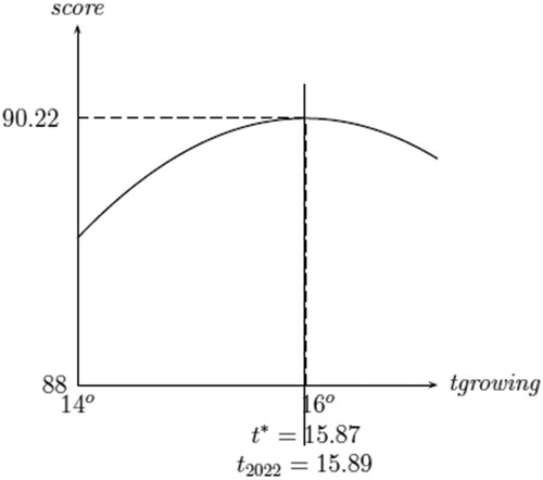The marginal effect is: (3) $Marginaleffect=\${\displaystyle \frac{\mathrm{\partial }Score}{\mathrm{\partial }tgrowing}={\text{β}}_1+2{\text{β}}_{2}tgrowing}$(3) While we expect to find a positive coefficient for the linear term, ${\text{β}}_1$, and a negative coefficient for the quadratic-term, ${\text{β}}_2$, we have no hypothesis for the sign of the marginal effect. In fact, one of the main points of our research agenda is to identify this sign. If we have a positive marginal effect, we can expect wine scores to go up at least in the short term as temperatures rise, while a negative overall marginal effect indicates that the current temperature is already past the optimal level. Figure 2 shows an example of how the regression results can be illustrated in a 2-dimensional graph that maps the average wine score to the growing-season temperature.⁹

Figure 2. Estimated regression model 2 without trend for Marlborough Sauvignon Blanc, calibrated for 2022 forecast levels of tgrowing, dormantrain and harvestrain.

Because we have observations from seven wine regions, all with their unique current temperature, instead of reporting the marginal effects for each region, we report the implied optimal temperature for each variety. This is found by setting equation (3) equal to zero and solving for the temperature variable: (4) $tgrowin{g}^{\ast }=-{\displaystyle \frac{{\text{β}}_1}{2{\text{β}}_2}}$(4) Note that Equation (4) gives the optimal temperature only when the coefficients have the expected signs and thus when the relationship between the score and the growing season temperature is concave. When the coefficients are contrary to expectation, Equation (4) gives the temperature that minimises the score. The optimal temperature for a variety in (4) can be compared with the current temperatures of the wine regions to understand the scope for the region to produce that variety into the future. If the optimal temperature in (4) is larger than the current temperature in a given region, we can expect the average quality of the wine to increase for the time being with further increases in temperature. This is equivalent to finding a positive marginal effect in (3). Similarly, if the optimal temperature is below the current temperature in the region, the marginal effect is negative and we have already surpassed the point where climate change starts to deteriorate average wine quality for the given variety and region. In our example result illustrated in Figure 2, the optimal temperature is 0.02 °C above the 2022 forecast temperature, suggesting that the average quality for Sauvignon Blanc has just started its decline. After we discuss the main findings in Section 7, we briefly discuss where the optimal temperatures for key varieties are with respect to the current average temperatures in the New Zealand wine regions.

6. Summary statistics

Table 3 contains the summary statistics of the climatic variables used in the research for New Zealand as a whole and for its seven main wine regions, organised from North to South. The last four columns contain the results of regressing each climatic variable on the time trend¹⁰ allowing for an understanding of any systemic changes over time. The coefficient for the variable trend measures the annual growth of the climatic variable of concern. We can see that all wine regions except Wairarapa have experienced a significant increase in the growing season average temperature of 0.04-0.06 °C per year. Auckland, Canterbury and Otago have experienced a significant growth in the difference between the growing season maximum and minimum temperatures, tgrowingdiff. Nelson has experienced a mildly significant increase in the harvest rain but other rainfall variables have been stationary. This suggests that climate change in New Zealand, at the moment at least, is mostly manifested in the positive trend of the average growing-season temperature, with some regions also experiencing larger daily fluctuations between the minimum and the maximum temperatures. The last column presents the 2022 forecast value of the climatic variable, obtained from the regression results.¹¹ This 2022 forecast is used in Section 7 as a measure of the region’s current temperature to compare with our model’s prediction of the optimal temperature.

Table 3. Summary statistics of the temperature and rainfall variables for 2002–2016 including time trend and 2022 prediction, for New Zealand and main wine regions.

Variables	N	Summary statistics				Regression results
		mean	sd	min	max	Constant	trend	R2	2022
New Zealand
tgrowing	14,763	15.67	0.884	11.35	19.59	15.49***	0.0258	0.125	16.01
tgrowingdiff	14,763	11.50	2.374	5.470	15.83	10.84***	0.0847***	0.523	12.53
dormantrain	14,763	341.6	158.6	63.70	726.8	310.1***	3.016	0.029	370.4
harvestrain	14,763	74.96	54.54	5.900	316.6	67.84***	1.088	0.032	89.60
Auckland
tgrowing	542	17.90	0.474	17.03	19.59	17.54***	0.0601**	0.380	18.74
tgrowingdiff	542	7.128	0.652	5.470	9.670	6.528***	0.0898***	0.698	8.325
dormantrain	542	561.9	86.50	355.2	725.6	517.2***	8.311	0.186	683.4
harvestrain	542	64.94	53.67	7.600	245.8	97.78***	−3.344	0.070	30.89
Hawke's Bay
tgrowing	2,495	16.62	0.368	15.95	17.30	16.21***	0.0548**	0.386	17.31
tgrowingdiff	2,495	10.06	0.533	8.890	11.26	9.715***	0.0388	0.101	10.49
dormantrain	2,495	400.6	89.97	248.6	552.3	439.7***	−6.898	0.105	301.8
harvestrain	2,495	125.9	69.31	51	316.6	109.6**	3.264	0.037	174.9
Wairarapa
tgrowing	1,167	16.62	0.362	15.77	17.21	16.43***	0.0242	0.085	16.91
tgrowingdiff	1,167	7.113	0.303	6.430	7.680	6.930***	0.0210	0.077	7.350
dormantrain	1,167	495.2	155.1	230.7	726.8	498.2***	−2.276	0.004	452.6
harvestrain	1,167	64.27	41.38	14.40	166.2	61.90**	0.230	0.001	66.50
Nelson
tgrowing	1,049	15.79	0.351	15.26	16.62	15.48***	0.0514**	0.367	16.50
tgrowingdiff	1,049	9.110	0.329	8.310	9.780	8.869***	0.0371	0.161	9.612
dormantrain	1,049	439.6	94.16	274.6	592.7	394.2***	4.678	0.048	487.7
harvestrain	1,049	115.8	64.18	21.60	296.6	65.24*	8.204*	0.260	229.3
Marlborough
tgrowing	5,900	15.40	0.334	14.70	15.94	15.10***	0.0397*	0.256	15.89
tgrowingdiff	5,900	12.42	0.527	11.07	13.28	11.96***	0.0566	0.166	13.09
dormantrain	5,900	346.9	134.9	177.8	709.1	245.2***	11.59	0.149	476.9
harvestrain	5,900	76.28	35.16	21.60	130.8	70.53***	0.961	0.015	89.75
Canterbury
tgrowing	1,122	14.38	0.421	11.35	14.90	13.98***	0.0514**	0.343	15.01
tgrowingdiff	1,122	11.06	0.502	9.210	13.34	10.39***	0.0732*	0.263	11.85
dormantrain	1,122	297.9	93.99	188.6	452.9	233.3***	6.594	0.103	365.2
harvestrain	1,122	39.43	24.94	5.900	123.2	29.33**	1.763	0.093	64.60
Otago
tgrowing	2,488	14.96	0.388	11.35	15.28	14.64***	0.0404**	0.337	15.45
tgrowingdiff	2,488	15.00	0.436	12.36	15.83	14.58***	0.0499*	0.208	15.57
dormantrain	2,488	128.5	42.05	63.70	399.4	107.0***	2.618	0.090	159.3
harvestrain	2,488	26.80	13.68	5.900	47.80	18.72**	1.043	0.103	39.57

Table 4 shows the summary statistics of the wine scores by grape variety and by region. It also shows the regression results where the annual average score per variety or region, respectively, is regressed on the time trend to understand changes in the average wine scores over time. The top half of the table shows that the average wine was rated at 90 points and that all grape varieties have experienced significant rating growth over the study period. The bottom half of the table shows that wines from all regions have grown in quality over the study period although the growth has been the slowest for Marlborough, which is the most important wine region in New Zealand in terms of size.

Table 4. Summary statistics of wine scores by variety and region, including trend, for 2002, 2016 and 2002-2016.

Variables	2002–2016						Regression
	N	Mean	sd	Min	Max	Constant	trend	R2
Pinot Noir	4,216	90.26	3.711	83	99	88.42***	0.239***	0.709
Syrah	851	91.03	3.710	83	99	89.26***	0.184**	0.334
Chardonnay	2,513	89.94	3.645	83	100	88.28***	0.243***	0.867
Merlot	484	88.11	3.464	83	96	86.84***	0.167**	0.264
Sauvignon Blanc	3,068	89.58	3.478	83	97	87.20***	0.286***	0.714
Riesling	1,866	90.53	3.536	83	99	88.28***	0.301***	0.838
Pinot Gris	1,765	89.74	3.261	83	98	88.43***	0.151***	0.591
Total	14,763	90.01	3.608	83	100	88.19***	0.235***	0.812
Auckland	542	89.28	3.938	83	97	86.53***	0.408***	0.784
Hawke's Bay	2,495	89.32	3.693	83	99	87.74***	0.203***	0.542
Wairarapa	1,167	91.18	3.494	83	99	89.10***	0.259***	0.633
Nelson	1,049	89.11	3.467	83	100	86.86***	0.304***	0.790
Marlborough	5,900	89.85	3.542	83	98	88.56***	0.164***	0.545
Canterbury	1,122	90.10	3.612	83	97	88.10***	0.258***	0.643
Otago	2,488	91.02	3.337	84	98	88.95***	0.261***	0.831
New Zealand	14,763	90.01	3.608	83	100	88.19***	0.235***	0.812

7. Results and discussion

In this section, we report the summary results of the product-level and the vintage regressions and compare how well the two approaches work to identify optimal temperatures for the main varieties grown in New Zealand. We also discuss how these results vary between the seven varieties studied and the different models used, which allows us to make some general conclusions about lessons learned in this study.

For each variety, we have eight regressions using product-level data and four regressions using vintage data. Our focus is on the summary results, found in Table 5, where we present coefficient estimates and significance levels for all the temperature variables, the R² value of the regression and the predicted optimal temperature, tgrowing*, from Equation (4). The purpose of this section is to look at the high-level results that indicate whether the models are useful for identifying the optimal temperature for each variety. The full results are available from the authors for those interested in seeing more detail.

Table 5. Summary results for all varieties.

Note: Green and white: coefficients for tgrowing and tgrowingsq have expected signs and results are significant at 1% (dark green), 5% (middle green) or 10% (light green) levels or not significant (white). Red: coefficients for tgrowing and tgrowingsq are inconsistent with expectation. Red circle: the optimal temperature point estimate is within the optimal temperature range from Jones (2015), given under the variety name.

In Table 5, Columns 1 and 2 present the results of the FE model with regional fixed effects of Model 1 and Model 2, respectively. Columns 3 and 4 add the trend variable to columns 1 and 2, respectively. Columns 5–8 are the same as columns 1–4 but for the FE model with product-level fixed effects. Columns 9 and 10 presents the results of Model 1 and Model 2 using the vintage data, while Columns 11 and 12 present these results with the trend variable. The temperature band underneath each variety’s name on the left of the table is the optimal temperature band from Jones (2015) that we use to gauge how plausible our temperature predictions are.

We use colour codes to help the reader digest these high-level results. The cells highlighted in red have signs of the linear and the quadratic temperature terms contrary to expectations. The ‘red’ results are not plausible because they suggest a convex relationship between the wine score and the growing-season temperature, which means that extreme cold and extreme hot weather would produce the best wines. The white cells indicate results where the temperature coefficient signs are consistent with expectations but have insignificant coefficients. The green cells indicate results where the temperature coefficients are not only consistent with our hypothesis but are also statistically significant – the darker the green the more significant are the coefficients.¹² The red circle around tgrowing* indicates that our estimate for the optimal growing-season temperature for the variety is within the band of optimal temperatures given by Jones (2015) and as such deemed plausible by us.

Overall, we find that the results are substantially more robust and reliable when we use vintage data than when we use the product-level data. When we use the vintage data in columns 9-12, 100% of the results have the expected signs, 64% (18/28) also have significant coefficients and 86% (24/28) provide plausible optimal temperature predictions. When we use product-level data in columns 1-8, only 50% (28/56) of the results have the expected signs, just 9% (5/56) have significant coefficients and 21% (13/56) provide plausible optimal temperature predictions. It seems that the process of averaging the scores for each region and year removes some of the subjectivity that is present in the product-level data, making it easier to identify the underlying relationship between the quality of wine and weather. Despite drastically reducing the size of the sample, we get results that are consistent and seemingly useful for understanding the long-term prospects of each variety in a given region. Furthermore, the R² values of the vintage regressions are much higher than those found with product-level data.

We fail to find any useful results for Merlot – all the product-level results in columns 1–8 have coefficients that are opposite to what we would expect, and the vintage-level results have the expected coefficient signs but provide implausible optimal temperature estimates. For Syrah, Sauvignon Blanc, Riesling and Pinot Gris, the vintage results have the expected signs, are mostly significant and provide plausible predictions while the product-level results either have signs contrary to expectations or are insignificant, although some of the results still provide plausible predictions. The only variety for which the product-level data appears to work somewhat better than the vintage data is Chardonnay for which three of the product-level and none of the vintage level results are significant. However, the vintage results still provide plausible point estimates for the optimal temperature. Other common themes are that the models using regional fixed effects outperform those using product-level fixed effects, and the models with the trend variable usually outperform the models without a trend. The main issue with using product-level fixed effects is that the number of observations of each product reduces to 15 or fewer.

The results for tgrowingdiff, which measures the average difference between the daily max and the daily min temperatures during the growing season, do not fully conform with the hypothesis from Oczkowski (2016) that its coefficient should be negative. Furthermore, the coefficient often changes signs when we add the trend variable to a regression, suggesting that incorporating the trend variable may introduce issues with multicollinearity.

The significance and plausibility of our results seem to be ‘colour-blind’ with respect to red and white wine types – in the vintage model our worst results are for Merlot and the best for Syrah and Pinot Noir, all of which are red varieties. Of note is that Merlot has the smallest sample of rated wines in our dataset of all the varieties, which likely plays some role in why the results are imprecise and implausible. Sadras et al. (2007) found significant results for the Australian red varieties but not the white ones. This is consistent with Australia’s focus on red varieties that dominate the list of rated wines.

Figure 3 and Figure 4 summarise our findings of the optimal temperature estimates and their plausibility. Figure 3 plots the ‘white’ and ‘green’ point estimates of the optimal temperatures from the product-level results in Table 5. The point estimates are plotted against the optimal temperature band from Jones (2015), shown as the green cross-hatched range for each variety. Figure 4 does the same from the vintage results. In Figure 3, a number of the point estimates for Chardonnay and Syrah are well above those found in Jones (2015) and are clearly implausible. Furthermore, the product-level regressions do not provide any point estimates for Merlot. In Figure 4 that plots the vintage results, only the estimates for Merlot are outside of the Jones range and we have plausible estimates for all the other varieties. This again demonstrates that the vintage results provide more accurate predictions for the optimal temperature ranges for the varieties grown in New Zealand.

Figure 3. Predicted growing season average temperatures for the wine regions and the optimal growing season temperature bands for each variety from product-level results.¹³

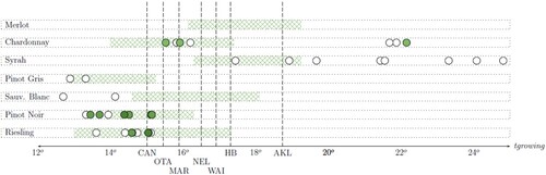
Figure 4. Predicted growing season average temperatures for the wine regions and the optimal growing season temperature bands for each variety from vintage-level results.¹⁴

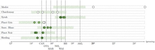
We have also included in Figure 4 the 2022 predicted growing season temperatures for each region from Table 3, represented by the vertical lines, to understand how different regions are currently suited for the varieties studied. We can see that Pinot Noir and Riesling, the most important varieties for Canterbury, have an optimal temperature range that fits well within the current temperature range of Canterbury. Canterbury is also well suited for Pinot Gris and Chardonnay and becoming more ideal for Sauvignon Blanc. Figure 4 suggests that Otago’s current temperature is already moving towards the top range of what is optimal for Pinot Noir, Riesling and Pinot Gris, its main varieties, at least given the current wine-making style. Figure 4 also suggests that the current climate in Otago is becoming more ideal for Sauvignon Blanc and Chardonnay. Marlborough’s current temperature is ideal for its most important variety, Sauvignon Blanc, as well as Chardonnay, but too warm for Pinot Noir, Riesling and Pinot Gris. Nelson is too warm for its main varieties, Pinot Noir, Sauvignon Blanc, Riesling and Pinot Gris but is well-suited for Chardonnay. Wairarapa is similarly too warm for its main varieties, Pinot Noir, Sauvignon Blanc, Riesling and Pinot Gris, but is ideal for Chardonnay and starting to be ideal for Syrah. Hawke’s Bay is ideal for Syrah but already too warm for Chardonnay and Sauvignon Blanc. Last, we have no varieties that we found to be ideal for Auckland, but based on Jones (2015), its temperature is ideal for Merlot and Syrah, albeit with a different style than what is currently produced in New Zealand. It can also successfully produce Cabernet Sauvignon and Zinfandel that are not featured in Figure 2 because they are not widely produced in New Zealand and thus we did not have sufficient observations to study their suitability in New Zealand.

The fact that the temperature ranges from Jones (2015) extend in most cases beyond our point estimates suggest that there is further scope for success for most of the varieties in most of the regions, with some adjustments in wine-making styles. However, the temperatures in Nelson, Wairarapa, Hawke’s Bay and Auckland are too warm for Pinot Noir, and the temperatures in all the regions but Canterbury are too warm for Pinot Gris even when using the Jones (2015) band.

8. Conclusion

We used individual wine ratings from an extensive list of wines rated by Bob Campbell in 2002–2016 to investigate the feasibility of using such an expert-rating dataset for climate-change research in New Zealand. We investigated a function that linked the growing-season temperature to the wine quality separately for the seven most rated single-variety wines in the dataset. We used both product-level and constructed vintage-level data to see how often our models provide plausible results. Last, we compared the optimal temperature predictions to the (predicted) 2022 growing-season temperature to discuss how each region’s production mix is currently matched to its climate, and what changes might be needed to ensure future success as the climate continues to warm up.

Our results suggest that the product-level data is not very reliable – only 50% of the results have expected signs and only 21% provide point estimates for the varietal optimal temperature that fits within the range provided by Jones (2015). The regional fixed effects model tends to work better than the product fixed effects model. The vintage-level regressions give superior results. 100% of the results have expected signs and 86% – all the varieties except Merlot – provide plausible optimal temperature predictions.

Our results contribute to the literature that has found that some varieties, or even regions, do not have a clear link between climate and quality. Examples of such studies include, amongst others, Oczkowski (2016) who found a convex relationship between weather and quality for Riesling and Semillon, and Jones et al. (2005), who found that the relationship between climate and the quality of wine is ‘less clear’ for the New World wine regions than for the Old World wine regions. Using the vintage data that was constructed from product-level data, we obtained results that show a clear positive, concave relationship between the wine quality and the growing season temperature with a very plausible optimal temperature estimate for most of the main varieties grown in New Zealand. This suggests that expert ratings can be very useful in helping wine producers understand and adapt to the effect of climate change.

Disclosure statement

No potential conflict of interest was reported by the author(s).

Notes

1 According to the Intergovernmental Panel on Climate Change [IPCC] (2007), climate change is a statistically significant variation in either the mean state or the variability of climate that persists for an extended period, typically decades or longer.

2 https://www.therealreview.com/wines/.

3 https://cliflo.niwa.co.nz/.

4 https://www.nzwine.com/en/region/.

5 Campbell originally scored using a 20-point system but later switched to the 100-point scale used by Gourmet Traveller Wine as well as Robert Parker, using a mathematical model to convert his earlier scores into ones that are compatible with the 100-point system.

6 For those interested, this was the 2014 Moutere Chardonnay from the Neudorf Vineyard, located in the Nelson wine region.

7 For example, Felton Road Wines has 12 wine labels, or products, in the dataset, including four different labels of Chardonnay, five of Pinot Noir and three of Riesling, but not all of these were made and/or tasted each year.

8 When constructing Figure 2, we used the vintage regression coefficients of Model 2 without trend for Sauvignon Blanc, where the remaining variables are given at their 2022 forecast values for Marlborough. This model suggests that the 2022 growing season temperature for Marlborough at 15.89 °C is very close to the optimal temperature for Sauvignon Blanc.

9 The variable trend is set to equal 0 in 2002 and increases by one per year from there on.

10 Specifically, the 2022 forecast is equal to the constant + trend coefficient *(2022-2002).

11 Dark green: either both terms are significant at 1% or one is significant at 1% and the other at 5%; Medium green: either both terms are significant at 5% or one is significant at 5% and the other at 10%; Light green: either both terms are significant at 10% or one is significant at 10% and the other is not significant.

12 AKL=Auckland; HB=Hawke's Bay; WAI=Wairarapa; NEL=Nelson; MAR=Marlborough; CAN=Canterbury, OTA=Otago. The cross-hatch represents the optimal temperature range from Jones (2015). Observation not shown on the graph: Chardonnay (29.56°).

13 Regions are as in Figure 3. Observations not shown on the graph: Merlot (32.44° and 49.63°).

References

- Ashenfelter, O. (2008). Predicting the quality and prices of Bordeaux wines. The Economic Journal, 118(529), F174–F184. https://doi.org/10.1111/j.1468-0297.2008.02148.x
- Ashenfelter, O. (2010). Predicting the quality and prices of Bordeaux wines. Journal of Wine Economics, 5(1), 40–52. https://doi.org/10.1017/S193143610000136X
- Ashenfelter, O., Ashmore, D., & Lalonde, R. (1995). Bordeaux wine vintage quality and the weather. Chance, 8(4), 7–14. https://doi.org/10.1080/09332480.1995.10542468
- Ashenfelter, O., & Jones, G. (2013). The demand for expert opinion: Bordeaux wines. Journal of Wine Economics, 8(3), 285–293. https://doi.org/10.1017/jwe.2013.22
- Ashenfelter, O., & Storchmann, K. (2016). Climate change and wine: A review of the economic implications. Journal of Wine Economics, 11(1), 105–138. https://doi.org/10.1017/jwe.2016.5
- Baciocco, K. A., Davis, R. E., & Jones, G. V. (2014). Climate and Bordeaux wine quality: identifying the key factors that differentiate vintages based on consensus rankings. Journal of Wine Research, 25(2), 75–90. https://doi.org/10.1080/09571264.2014.888649
- Blanco-Ward, D., Monteiro, A., Lopes, M., Borrego, C., Silveira, C., Viceto, C., Rocha, A., Ribeiro, A., Andrade, J., Feliciano, M., Castro, J., Barreales, D., Neto, J., Carlos, C., Peixoto, C., & Miranda, A. (2019). Climate change impact on a wine-producing region using a dynamical downscaling approach: Climate parameters, bioclimatic indices and extreme indices. International Journal of Climatology, 39(15), 5741–5760. https://doi.org/10.1002/joc.6185
- Byron, R. P., & Ashenfelter, O. (1995). Predicting the quality of an unborn Grange. The Economic Record, 71(212), 40–53. https://doi.org/10.1111/j.1475-4932.1995.tb01870.x
- Corsi, A., & Ashenfelter, O. (2019). Predicting Italian wine quality from weather data and expert ratings. Journal of Wine Economics, 14(3), 234–251. https://doi.org/10.1017/jwe.2019.41
- Corte-Real, A., Borges, J., Cabral, J. S., & Jones, G. V. (2015). Partitioning the grapevine growing season in the Douro Valley of Portugal: accumulated heat better than calendar dates. International Journal of Biometeorology, 59(8), 1045–1059. https://doi.org/10.1007/s00484-014-0918-1
- Corte-Real, A., Borges, J., Cabral, S., & Jones, V. (2017). A climatology of Vintage Port quality. International Journal of Climatology, 37(10), 3798–3809. https://doi.org/10.1002/joc.4953.
- Goldstein, R. (2008, Aug 15). What does it take to get a Wine Spectator award of Excellence? Blindtaste. http://blindtaste.com/2008/08/15/what-does-it-take-to-get-a-wine-spectator-award-of-excellence/.
- Grifoni, D., Mancini, M., Maracchi, G., Orlandini, S., & Zipoli, G. (2006). Analysis of Italian wine quality using freely available meteorological information. American Journal of Enology and Viticulture, 57(3), 339–346. https://doi.org/10.5344/ajev.2006.57.3.339
- Haeger, J. W., & Storchmann, K. (2006). Prices of American pinot noir wines: Climate, craftsmanship, critics. Agricultural Economics, 35(1), 67–78. https://doi.org/10.1111/j.1574-0862.2006.00140.x
- Halliday, J. (2014). Australian wine companion (2015 ed). Hardie Grant Books.
- Hannah, L., Roehrdanz, P. R., Ikegami, M., Shepard, A. V., Shaw, M. R., Tabor, G., Zhie, L., Marquet, P. A., & Hijmans, R. J. (2013). Climate change, wine, and conservation. Proceedings of the National Academy of Sciences, 110(17), 6907–6912. https://doi.org/10.1073/pnas.1210127110
- Hodgson, R. T. (2008). An examination of judge reliability at a major U.S. wine competition. Journal of Wine Economics, 3(2), 105–113. https://doi.org/10.1017/S1931436100001152
- Intergovernmental Panel on Climate Change. (2007). Climate change: The physical science basis. Summary for policymakers contribution of working Group I to the fourth assessment report.
- Jones, G. V. (2015, Aug 12). Climate, grapes, and wine: Terroir and the importance of climate to winegrape production. GuildSomm Feature Articles. https://www.guildsomm.com/public_content/features/articles/b/gregory_jones/posts/climate-grapes-and-wine?CommentId=a160ab2a-2bb7-44e5-8ce6-b75702681dd1
- Jones, G. V., & Davis, R. E. (2000). Climate influences on grapevine phenology, grape composition, and wine production and quality for Bordeaux, France. American Journal of Enology and Viticulture, 51(3), 249–261. https://doi.org/10.5344/ajev.2000.51.3.249
- Jones, G. V., White, M. A., Cooper, O. R., & Storchmann, K. (2005). Climate change and global wine quality. Climatic Change, 73(3), 319–343. https://doi.org/10.1007/s10584-005-4704-2
- Mozell, M. R., & Thach, L. (2014). The impact of climate change on the global wine industry: Challenges and solutions. Wine Economics and Policy, 3(2), 81–89. https://doi.org/10.1016/j.wep.2014.08.001
- New Zealand Wine Growers Association. (2022). Annual Report 2022. https://www.nzwine.com/en/media/statistics/annual-report
- Oczkowski, E. (2016). The effect of weather on wine quality and prices: An Australian spatial analysis. Journal of Wine Economics, 11(1), 48–65. https://doi.org/10.1017/jwe.2015.14
- Ramirez, C. D. (2008). Wine quality, wine prices, and he weather: Is Napa “different”? Journal of Wine Economics, 3(2), 114–131. https://doi.org/10.1017/S1931436100001164
- Reuter, J. (2009). Does advertising bias product reviews? An analysis of wine ratings. Journal of Wine Economics, 4(2), 125–151. https://doi.org/10.1017/S1931436100000766
- Sadras, V. O., Soar, C. J., & Petrie, P. R. (2007). Quantification of time trends in vintage scores and their variability for major wine regions of Australia. Australian Journal of Grape and Wine Research, 13(2), 117–123. https://doi.org/10.1111/j.1755-0238.2007.tb00242.x
- Storchmann, K. (2012). Wine economics. Journal of Wine Economics, 7(1), 1–33. https://doi.org/10.1017/jwe.2012.8
- Tate, A. B. (2001). Global warming’s impact on wine. Journal of Wine Research, 12(2), 95–109. https://doi.org/10.1080/09571260120095012
- Turner, J., Bindschadler, R., Convey, P., Di Prisco, G., Fahrbach, E., Gutt, J., & Summerhayes, C. (2009). Antarctic climate change and the environment. The International Council for Science, Scientific Committee on Antarctic Research.
- van Leeuwen, C., & Darriet, P. (2016). The impact of climate change on viticulture and wine quality. Journal of Wine Economics, 11(1), 150–167. https://doi.org/10.1017/jwe.2015.21
- Wood, D., & Anderson, K. (2006). What determines the future value of an icon wine? New evidence from Australia. Journal of Wine Economics, 1(2), 141–161. doi:10.1017/S1931436100000171