Osmotic pressure estimation using the Pitzer equation for forward osmosis modelling

ABSTRACT

Forward osmosis (FO) has received widespread recognition in the past decade due to its potential low energy production of water. This study presents a new model analysis for predicting the water flux in FO systems when inorganic-based draw solutions are used under variable experimental conditions for using a laboratory scale cross-flow single cell unit. The new model accounts for the adverse impact of concentration polarization (both ICP and ECP) incorporating the water activity by Pitzer to calculate the bulk osmotic pressures. Using the water activity provides a better correlation of experimental data than the classical van’t Hoff equation. The nonlinear model also gave a better estimate for the structural parameter factor (S) of the membrane in its solution. Furthermore, the temperature and concentration of both the draw and feed solutions played a significant role in increasing the water flux, which could be interpreted in terms of the mass transfer coefficient representing ECP; a factor sensitive to the hydraulics of the system. The model provides greatly improved correlations for the experimental water fluxes.

GRAPHICAL ABSTRACT

KEYWORDS:

• Forward osmosis
• draw solution
• osmotic pressure
• water flux modelling
• membrane separation

1. Introduction

The stress on water resources to match the ever-growing demand for water is very well documented in the literature due to population growth, increased industrial activities and climate change. Desalination, a general term used for processes that removes salts from water, is used extensively around the globe for the purpose of increasing the production of high-quality water, with reverse osmosis and multi stage flash evaporation (MSF) being the two most widely used technologies [1,2]. In RO, hydraulic pressure is applied to push the water across a semipermeable membrane; a process associated with reported high energy requirements, membrane fouling and other costs linked with operations and pretreatment, making the need for more energy-efficient membrane processes an important area of focus for researchers [3,4]. Compared to thermal and RO separation processes, many researchers now view FO as a low energy alternative technology, that also offers minimal chemical discharges and low hydraulic pressure and temperature requirements. Linares et al. [2] presented an extended review regarding the recent niches in seawater desalination. In this review, it was reported that the main reason behind the low energy requirement in FO stems from the fact that this process is based on mimicking naturally occurring phenomena: osmosis; a process omnipresent in all living biological cells with almost no external hydraulic pressure requirements. In FO systems, a solution with higher concentration than the feed solution (termed ‘draw’ solution) is utilized to create a concentration variance that drives pure water through the semipermeable membrane. The semipermeable membrane permits molecules of water only to pass through the membrane while rejecting the salts present in the solute. Intensive research has been taking place to assess the suitability of many materials in the role of forward osmosis membranes [5–8]. The draw solution (DS), based on its intended end use, may be treated or diluted and in which case, the treatment process energy requirements should also be taken into account. In addition to its applications in seawater and brackish water desalination, recent reports employed FO with biological wastewater treatment especially those associated with osmotic membrane bioreactors [1,9–11].

A major key factor in the effectiveness of the FO processes is the selection of the draw solution. Organic and inorganic, single and multiple solute solutions are known to impact water flux and process behaviour [1,2,12,13]. In general, a good draw needs to process a higher osmotic pressure compared to the feed solution (FS) in addition to being easily recovered. From the variety of inorganic salts used, NaCl, KCl, CaCl₂ are very common due to their abundance and low costs in addition to ease of recovery. A number of draw solution materials have been investigated to improve the membrane performance [14–18]. Liu et al. [9] studied the effects of ammonium bicarbonate mixed with eight salts and their impact on flux behaviour. The type of membrane used and the flow mode are also major parameters influencing the performance of the FO process [1,3]. The asymmetric membranes applied in FO uses are made from a variety of materials but, in general, all have a high-density material layer formed on top of a more porous support layer [1–3]. This results in two types of concentration polarization (a phenomena associate with membrane processes) namely: internal concentration polarization (ICP) (in the porous support layer of the membrane) and external concentration polarization (ECP) (occurring at the feed–membrane and draw solution membrane interfaces) both hindering the performance of the membrane and consequently reducing the driving force. Taking into account the complexity of the system and the influence of such variables (membrane characteristics, the draw solution characteristics, operating conditions), modelling of the water flux, especially when taking into account the mass transfer phenomenon across the membrane, may offer a powerful tool to estimate the water flux in the system at various conditions. Water flux modelling in forward osmosis has been established and reported with models developed and applied using different assumptions and levels of complexity [1,12]. For instance, McCutcheon et al. [19] proposed one of the earlier models, which was used by some researchers as reported in the work of Shim et al. [20]. In this model, water permeability through the membrane was considered, but no consideration was given to the salt permeability. Later models mostly considered this factor, as in the work reported by Chanukya et al. [21]. Some modelling works neglected the effect of ECP, even though it has been proven to influence the flux widely [2]. In all cases, most modelling works applied equations that predicted the flux based on the assumption that the relation between the osmotic pressure and solution concentration is linear, an approximation that will be investigated in this work. Accordingly, the aim of this study is to investigate the ICP and ECP phenomena and their effect on water flux in forward osmosis through utilizing a numerical model that considers both effects, as well as the non-ideality of feed and draw solutions when calculating the bulk osmotic pressure. The linear assumption embedded in the van’t Hoff equation is replaced by estimating the osmotic pressure using water activity. Moreover, the effect of osmotic pressure estimation on quantifying ICP and ECP parameters is considered. Finally, the model is verified by comparing the theoretical output to the experimental data produced using a single cell cross flow system with various draw solutions.

2. Experimental methods and materials

2.1. Feed and draw solutions

Deionized (DI) and saline water (0.1 M NaCl solution) have been used as the feed solutions and three different types of inorganic solutes (NaCl, KCl and CaCl₂) were used for the draw solution (DS). All solutions were supplied as pure reagents grade (Sigma Aldrich). DS solutions with concentrations of 1–5 mol/L (M) were prepared using standard chemical preparation procedures. The feed solution was mainly formed from DI water or simulated saline water with various concentrations. Various concentrations of NaCl were used depending on the required experimental conditions. Such solutions can easily represent brackish water used in Qatar. The properties of the solutions needed for the work were analysed in line with published experimental procedures describe elsewhere using Aspen plus which gave some of the important required thermodynamic properties [22].

2.2. Bench scale FO system and experimental protocol

The FO system used was a test bench scale model with a Sterlitech Sepa CF cell configured for Forward Osmosis supplies by Sterlitech (UK). The system is designed to test and evaluate a number of experimental parameters by simulating the flow dynamics across the membrane. The schematic flow diagram of this laboratory-based flat sheet cross flow membrane cell unit is given in Figure 1.

Figure 1. Experimental apparatus for FO cell and measuring draw solution

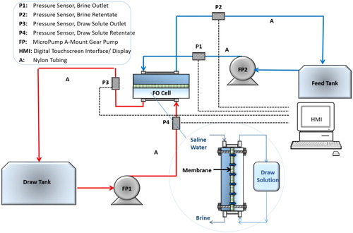
The cross flow membrane experimental unit cell has the following internal dimensions, 77 mm long, 26 mm wide and with a height of 3 mm. The membrane was a flat sheet hydrophilic thin film composite (TFC) type membrane with a support layer (Table 1) with a support layer (Table 1) was provided by Hydration Technologies Innovation (Inc, Albany, OR, USA). The specifications from the supplier state that the maximum temperature range for a stable operation of the membrane was 70°C and a maximum trans-membrane pressure of 70 kPa. Cross flow rate of 0.25–0.40 m/s. Two peristaltic micropumps were needed to move the draw and feed solutions around the system in a closed loop, 2 feed tanks with controlled temperature by heater/chiller and integrated a weighing balance (Sartorius weighing to monitor the variations in weight to record the variation). The feed and draw solution temperatures were held constant by the use of a water bath. Changes in weight of the water flux in the feed solution tank were measured using a digital balance and recorded by means of a data acquisition system to record the water flux. The temperature and pressure were constantly monitored throughout the experiments.

Table 1. Membrane properties.

Type	TFC		Water permeability	A (m/atm.d)	0.027
Active material	Polyamide		Solute permeability	B (m/d)	0.00028
Max pressure	600(psi)		Membrane dimensions	length (m)	0.077
Contact angle (°)	Active layer	45		Width (m)	0.026
	Support layer	45		Hight (m)	0.003
Zeta potential at pH 6	86 (mV)			dh (m)	0.0054
Operating pH range	2–12		Structural parameters
				Using van’t Hoff Osmotic pressure	S = 4.06 × 10^−4m (AL-FS)
					S = 3.45 × 10^−4m (AL-DS)
				Using Water Activity for Osmotic Pressure	S = 4,81 × 10^−4m (AL-FS)
					S = 4.38 × 10^−4m (AL-DS)

The experimental procedure starts with the cutting the required size of the membrane and fitting it appropriately in the cell. The membrane is then preconditioned in order to give reliable and consistent results for flux. The conditioning involves filling the feed tank with DI water and pressurizing the cell. The feed DI water temperature and system pressure used in the preconditioning of the membrane should be the same as those to be used in any of the experimental runs. The process takes usually 2 h to ensure full stabilization of the flux reading throughout the membrane is achieved. Once the system is rendered ready for use, the feed tank is filled with the appropriate solution ready for trail testing. The draw solution osmotic pressure was kept at a constant set value by topping up the concentrated draw solution in the draw solution tank. Upon the completion of each experiment, the system is flushed with DI water for 2 h before any new experiments take place. Experiments were repeated three times and average results were used in the calculations.

3. Theoretical modelling

3.1. Water flux equations

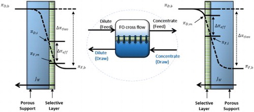
In FO, water flux is a phenomenon prompted by the osmotic pressure resulting from the solute concentration difference between the diluted feed solution (FS) and the draw solution (DS). Consequently, the DS pulls only the water through the membrane. The general water flux through the membrane (J_w) in a FO membrane is defined as [1,23]:(1) $J_w=A\left({\mathit{\pi }}_{\mathit{D}}-{\mathit{\pi }}_{\mathit{F}}\right)$(1) where A is the hydraulic permeability constant, ${\pi }_D$ is the draw solution osmotic pressure, and ${\pi }_F$ is the feed solution osmotic pressure. Predicting the water flux using Equation (1) does not take into account the concentration polarization effects on the osmotic difference or the driving force. When operating with the DS facing the active layer of the membrane and the FS facing the support layer (AL-DS mode, AL-FS, respectively [24,25]), the feed solution passing through the pores of the membrane will have higher concentration with time leading to internal concentration polarization (ICP). On the other hand, when operating with the porous layer facing the draw solution (AL-FS mode), the draw solution concentration decreases with time resulting in ICP. In both operational modes, the external concentration polarization (ECP) should also be accounted for. In all cases, as the concentration of the solution contacting the active layer increases, the importance of considering the ECP effect on the water flux increases. Equations (2) and (3) lump the effects of ICP and ECP together in predicting the water flux for the two operating modes [21,26]:(2) $\begin{array}{rl}& \left(\mathrm{A}\mathrm{L}-\mathrm{D}\mathrm{S}\right)\mathrm{m}\mathrm{o}\mathrm{d}\mathrm{e}:\\ & J_w=A\left[\frac{{\pi }_{D,b}exp\left({\displaystyle \frac{-J_w}{k}}\right)-{\pi }_{f,b}exp\left({\displaystyle \frac{J_{w}S}{D}}\right)}{1+{\displaystyle \frac{B}{J_w}\left[exp\left(\frac{J_{w}S}{D}\right)-exp\left(\frac{J_w}{k}\right)\right]}}\right]\end{array}$(2) (3) $\begin{array}{rl}& \left(\mathrm{A}\mathrm{L}-\mathrm{F}\mathrm{S}\right)\mathrm{m}\mathrm{o}\mathrm{d}\mathrm{e}:\\ & J_w=A\left[\frac{{\pi }_{D,b}exp\left({\displaystyle \frac{-J_{wS}}{D}}\right)-{\pi }_{f,b}exp\left({\displaystyle \frac{J_w}{k}}\right)}{1+{\displaystyle \frac{B}{J_w}\left[exp\left(\frac{J_w}{k}\right)-exp\left(\frac{-J_{wS}}{D}\right)\right]}}\right]\end{array}$(3)

In Equations (2) and (3), ${\pi }_{D,b}$ and ${\pi }_{f,b}$ are the osmotic pressure of the bulk draw and of the bulk feed solutions, respectively; k represents the mass transfer coefficient, with K as the solute resistivity. The mass transfer coefficient and the solute resistivity are the coefficients representing ECP and ICP respectively.

3.2. Osmotic pressure

In order to calculate the osmotic pressure in FO, the osmotic pressure equation proposed by van’t Hoff [2] is widely applied:(4) $\pi =nCRT$(4) where n is a van’t Hoff factor which is dependent on the number of particles in the solution, C is the solution molar concentration, R being the universal gas constant, and T is the ideal temperature. Equation (4) assumes a linear relation between the osmotic pressure and the solution concentration; it is used to derive Equations (2) and (3) and in most studies, it is used to calculate the bulk pressure when predicting the water flux theoretically. However, the linear assumption is mostly accurate for low concentration solutions or ‘ideal solutions’, and at higher concentrations the deviation from the ideal behaviour is more significant. For that reason, the bulk osmotic pressure in this work is calculated considering the water activity [27]:(5) $\pi =-\left(\frac{RT}{V}\right)\ln \left(a_w\right)$(5) where V is the water molar volume and a_w is the water activity. In this work the water activity is calculated using the Pitzer equation for electrolyte solutions [28,29]:(6) $a_w=\exp \left(-0.01802\oslash \sum _i{M}_i\right)$(6)

M_i is the molality of the solute in moles of solutes per kg of solvent and Φ is the osmotic coefficient calculated using Equations (7)–(11):(7) $\oslash -1=z_m{z}_{x}F+2m\left(\frac{v_m{v}_x}{v}\right)B_{mx}+2m^2\left[\frac{{\left(v_m{v}_x\right)}^{1.5}}{v}\right]C_{mx}$(7) (8) $F=-\frac{{0.3921}^{0.5}}{1+1.2I^{0.5}}$(8) (9) $I=0.5\sum _i{m}_i{z}_i^2$(9) (10) $\left|z_m{z}_x\right|=\frac{{\sum }_i{m}_i{z}_i^2}{{\sum }_i{m}_i}$(10) (11) $B_{mx}=B_{mx}\left(0\right)+B_{mx}\exp \left(-2.0I^{0.5}\right)$(11)

In the above equations, z_x and z_m are the charges of x and m ions and v_x and v_m are the respective stoichiometric coefficient of the ions, while B_mx (0), B_mx(1) and C_mx are the Pitzer equation constants specific to each solute.

3.3. Mass transfer coefficient computation

The ECP effect can be studied through the parameter k computed through the dimensionless Sherwood number using the following relation [19]:(12) $k=\frac{ShD}{d_h}$(12) where $d_h$ the hydraulic diameter of the membrane channel, Sh is the Sherwood number and D is the diffusion coefficient. $d_h$is calculated using the following equation:(13) $d_h=\frac{4\times Totalflowarea}{Totalwettedperimeter}=\frac{4\times W\times H}{W+H}$(13) where H and W represent the height and width of the rectangular channel, respectively.

The diffusion coefficient is a generic expression as expressed in Equation (13), irrespective of the chemical species. In this case, it is the coefficients for the solutes employed in this study (NaCl, KCl, CaCl₂).

In order to calculate Sherwood number, we have to predict the flow condition (laminar or turbulent), depending on the mean flow velocity, which is determined by using Reynolds number (Re). The flow is laminar when$Re\le 2100$, and turbulent when $Re>4000$; between 2100 ≥ Re ≥ 4000 we consider a ‘transitional region’ below turbulent flow; where Re is Reynolds number, which is obtained from the following equation:(14) $R{e}_F=\frac{d_h\nu {\rho }_F}{{\mu }_F}$(14) where $\nu ,\rho$ and $\mu$ indicate the liquid flow velocity, the liquid density and the dynamic viscosity, respectively.

When the flow is laminar, the following equation is applied:(15) $Sh=1.85{\left(ReSc\frac{d_h}{L}\right)}^{0.33}$(15) while for turbulent flow:(16) $Sh=1.85R{e}^{0.75}S{c}^{0.33}$(16) Where Sc is the Schmidt, which is obtained from the following equation(17) $Sc=\frac{v}{D}$(17) $\nu :$ is the kinematic viscosity

Equations (12)–(17) relate the mass transfer coefficient and the hydraulics of the system. The dependence of k on the solution properties (density and viscosity) and on the solution flow rate points out to the dependence of ECP effect on these factors. As a result, the severity of ECP could be mitigated through optimizing the operating conditions as will be illustrated in this paper.

3.4. Solute resistivity computation

The solute resistivity is the parameter quantifying the ICP phenomenon in the water flux model and it is defined as:(18) $K=\frac{t\tau }{D\epsilon }$(18) where t is the support layer thickness, τ is the tortuosity, and ε is the porosity. The term, $t\tau /\epsilon ,$ is known as the membrane structure parameter S. For a given membrane this value could be assumed constant and is determined using experimental flux data by the following form of Equations (2) and (3):(19) $\begin{array}{rl}& \left(\mathrm{A}\mathrm{L}-\mathrm{D}\mathrm{S}\right)\mathrm{m}\mathrm{o}\mathrm{d}\mathrm{e}:\\ & J_w=A\left[\frac{{\pi }_{D,b}exp\left({\displaystyle \frac{-J_w}{k}}\right)-{\pi }_{f,b}exp\left(J_{w}K\right)}{1+{\displaystyle \frac{B}{J_w}\left[exp\left(J_{w}K\right)-exp\left(\frac{J_w}{k}\right)\right]}}\right]\end{array}$(19) (20) $\begin{array}{rl}& \left(\mathrm{A}\mathrm{L}-\mathrm{F}\mathrm{S}\right)\mathrm{m}\mathrm{o}\mathrm{d}\mathrm{e}:\\ & J_w=A\left[\frac{{\pi }_{D,b}exp\left(-J_{w}K\right)-{\pi }_{f,b}exp\left({\displaystyle \frac{J_w}{k}}\right)}{1+{\displaystyle \frac{B}{J_w}\left[exp\left(\frac{J_w}{k}\right)-exp\left(-J_{w}K\right)\right]}}\right]\end{array}$(20)

4. Experimental results and temperature dependence of water flux

The purpose of having an accurate model to predict water flux in FO is to find optimum conditions that yield the high freshwater production. For this reason, this section aims at studying the water flux when varying some operating conditions, using the comprehensive model considering ICP and ECP effects and using water activity to estimate bulk osmotic pressure. The first operating condition studied is the temperature of both the draw and feed solutions.

The results in Figures 2 and 3 were obtained at NaCl concentrations of 1.5 and 0.1 M for the draw solution and the feed solution respectively, and a velocity of 0.408 m/s² for both solutions. When varying the temperature of the feed solution the draw solution temperature was fixed at 25°C as shown in Figure 2.

Figure 2. Flux for the two operating modes at different feed solution temperatures.

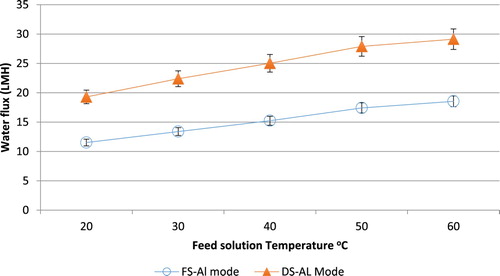
Figure 3. Flux for the two operating modes at different draw solution temperatures.

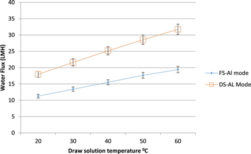
The same temperature was selected for the feed solution when varying the draw solution temperature as shown in Figure 3. When increasing the temperature of the feed solution or the draw solution, higher water flux values are achieved. Nonetheless, the magnitude at which the flux is increasing is not equal for both temperatures. More specifically, increasing the draw solution temperature has affected the water flux to a greater extent than the feed solution. In terms of the ICP and ECP phenomena, the solution temperature results in higher mass diffusivity values for the solutes, which in turn increases k and eventually reduces the effect of ECP. Moreover, increasing the mass diffusivity of a solution reduces the effect of ICP, by reducing K. The second factor studied in this section is the type of the draw solution used. Changing the solution type will change the properties and hence the solute behaviour. The error bars in the Figures represent a 6% experimental error as any experiment was repeated if the difference in the results was over a 5% error.

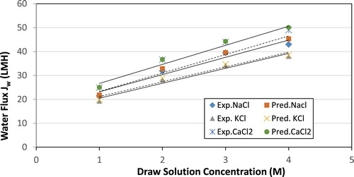
Figure 4 compares three draw solution, NaCl, KCl and CaCl₂ at various concentrations while keeping the feed solution NaCl concentration fixed at 0.1 M. Also, the temperature of both the draw and feed solutions were kept constant at 25°C. At these conditions, utilizing the CaCl₂ solution resulted in the highest water flux values at all concentrations followed by NaCl and finally KCl. In this particular scenario, the flux increase is not due to reducing the effect of the ECP as a result of increase in the diffusivity. In fact, the mass diffusivity coefficients for the three solutes in water are similar. On the other hand, the osmotic pressure of CaCl₂ is higher than that of NaCl and KCl due to the presence of three ions rather than two.

Figure 4. Water flux for different draw solutions at various concentrations (AL-DS mode).

5. Model solution and verification

The process used in the model formulation and solution is depicted in Figure 5. Input model data are used as in Table 2.

Figure 5. Flow chart of model formulation and solution.

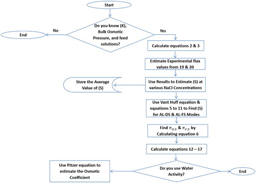
Table 2. Data used in model solution.

Feed solution		Draw solution
Solution type	NaCl	NaCl
n (=2 for NaCl)	2	2
T (K)	298.15	298.15
v (m/s)	0.408	0.408
Cf (mol/L)	0.1	Cd (mol/L)	0.7	1	2	3
π -bulk (atm)	4.893	πd -bulk (atm)	34.255	48.932	97.864	146.792
ρ (g/cm^3)	1.004	ρ (g/cm^3)	1.0253	1.038	1.077	1.126
μ (Pa s)	897.681	μ (Pa s)	945.91	972.3	1077.6	1207.8
D (m^2/s)	1.483 x10 ^−9	D (m^2/s)	1.48 × 10^−9	1.48 × 10^−9	1.38 × 10^−9	1.29 × 10^−9
Re	2.45 × 10^−3	Re	2.38 × 10^−3	2.34 × 10^−3	2.19 × 10^−3	2.05 × 10^−3
Sc	6.03 × 10^8	Sc	6.22 × 10^8	6.31 × 10^8	7.23 × 10^8	8.30 × 10^8
Sh	83.55	Sh	83.5	83.5	85.5	87.4
kf (m/s)	2.30 × 10^−5	kd (m/s)	2.30 × 10^−5	2.30 × 10^−5	2.19 × 10^−5	2.10 × 10^−5
		πd -memb (atm)	26.399	36.113	64.997	86.944
		πf -memb (atm)	6.349	6.631	7.232	7.888
		K	4.88 × 10^4	7.46 × 10^4	1.11 × 10^5	1.11 × 10^5
		Jw(m^3/m^2 s)	6.00 × 10^−6	7.00 × 10^−6	9.00 × 10^−6	1.10 × 10^−5
		e %	1.39%	1.91%	2.31%	2.11%

Equations (2) and (3) were solved for the water flux iteratively knowing the mass transfer coefficient (k), the bulk osmotic pressures for the draw and feed solution (π_D,b, π_F,b), and the membrane properties. The membrane related parameters A, B, and structural parameters S have constant values throughout the simulation for all conditions.

The A and B values employed were 0.027 m/atm.d and 2.8 × 10⁻⁴ m/d, respectively [19]. These values were reported for a membrane with the following dimensions, 77 mm long, 26, mm wide and with a height of 3 mm. To estimate the structural parameters experimental flux values were inputted into Equations (19) and (20) for both operating modes and solved for S. The experimental data used to estimate the S value are reported in Table 1. It also shows the experimental flux at various NaCl concentrations.

Basically, a single S value was obtained from each water flux recorded before all S values were averaged. This approach was applied to both the AL-DS and AL-FS mode data and a single average value was used for each mode respectively. Moreover, S was estimated by the van’t Hoff equation using the bulk pressure, and also using water activity and Equations (5)–(11). Finally, the S parameter values and the other membrane properties are summarized in Table 2.

Unlike the membrane properties listed in Table 2, the pressures and mass transfer coefficient are sensitive to changes in temperature, velocity and most importantly concentration. Accordingly, in the model solution, they have to be calculated for each simulation. In this work π_D,b and π_F,b are estimated considering the water activity coefficient calculated by the Pitzer Equation (6). For each run the operating conditions are specified, namely feed and draw solutions flow rates, temperature, concentrations, and solute type.

Then, after establishing these process variables, the density, viscosity and mass diffusivity of the feed and draw solution are obtained from Aspen Plus and utilized to calculate the mass transfer coefficient, k, using Equations (12)–(17). Also, the concentration and temperature of the solution are utilized in the osmotic bulk pressure calculation. When using water activity for calculating the osmotic pressure, the Pitzer equation is used to estimate the osmotic coefficient and the equation constants for a certain solute types B(0), B(1), and C_mx are taken from Pitzer et al. (1973) [29,30].

5.1. Model verification

The model equations considering ICP and ECP were solved using the methodology presented in Section 5.0 and the verification procedure is given in the flow chart depicted in Figure 6.

Figure 6. Flow chart of model verification.

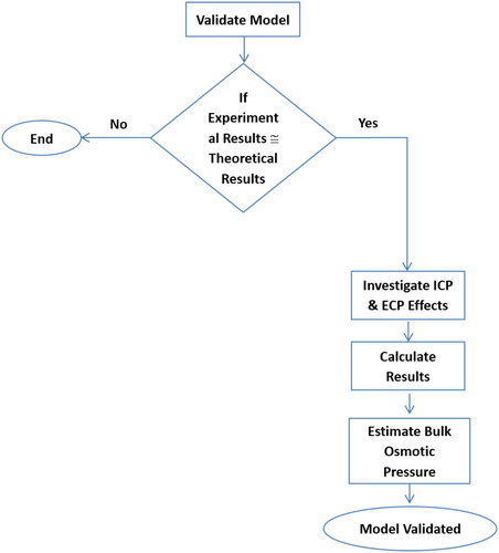
Prior to investigating the ICP and ECP effects, the model was validated by comparing its results with experimentally obtained values. The experimental data listed in Table 2 were considered, and the conditions provided in the same table were used to determine the water flux using the theoretical model. The bulk osmotic pressure was estimated through the water activity for both the draw and feed solutions. Also, the membrane structural parameters obtained by the same method were utilized.

Overall, the model prediction is in very good agreement with experimental values except for small deviations, specifically in the AL- FS mode at low concentrations (Figures 7 and 8).

Figure 7. Experimental vs. predicted flux for AL-FS operating mode at different feed solution (NaCl) concentrations.

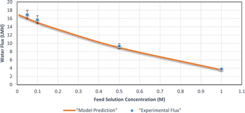
Figure 8. Experimental vs. predicted flux for AL-DS operating mode at different feed solution (NaCl) concentration.

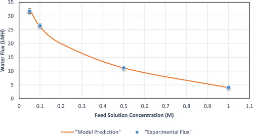
Other than validating the model equations, Figures 7 and 8 validate the non-ideal solution assumption made when calculating the bulk osmotic pressure. Furthermore, the influence of feed concentration on the water flux could be explained from the trends shown in the figures.

Having a feed with higher concentration will reduce the freshwater production. This observation may be explained because at a constant draw concentration, increasing the feed solution concentration will reduce the concentration difference, thus the driving force for the process. This trend was present and was predicted successfully in both modes (AL-FS and AL-DS). Yet, the trend is altered in each case, with the AL-FS mode having a linear decrease in water flux, while in the AL-DS mode the flux exhibited an exponential decrease. Furthermore, increasing the concentration of the feed solution reduces the mass transfer coefficient k, thus increasing the severity of ECP and reducing the freshwater production.

5.2. Effect of ideal solution assumption on water flux model prediction

In this section, the employment of the water activity as a factor in osmosis pressure calculations has been closely investigated by comparing it to the van’t Hoff equation, where the ideal solution assumption is made. To accomplish this goal, the osmotic pressure of NaCl solution at 25°C and different concentrations was estimated, using the water activity and the van’t Hoff equation. The results of both computations are compared in Figure 9. Using the van’t Hoff equation assumes a linear relation between the concentration and osmotic pressure thus the pressure increases linearly in Figure 9.

Figure 9. Osmotic pressure at different concentrations as calculated using two models

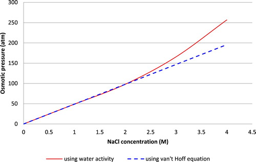
On the other hand, estimating the pressure through the water activity and Pitzer equation for osmotic coefficient will yield a non-linear trend. The pressure values reported for the later method are close to the van’t Hoff estimation at low concentrations, but are higher at more concentrated solutions. Secondly, it is important to investigate the influence of solution ideality on the water flux prediction.

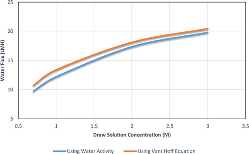
Figure 10, shows the water flux predicted theoretically; one based on assuming a linear relation between concentration and bulk osmotic pressure and one using the water activity for bulk osmotic calculations. Sodium chloride is used as feed solution and draw solution, the temperature of both solutions is fixed at 25°C, the velocity is 0.408 m²/s on both sides, and the feed solution concentration is set to be 0.1 M. While both assumptions, ideal and non-ideal, will have the same general trend, however using the van’t Hoff equation (ideal solution) will give overestimated flux values compared to using water activity (non-ideal solution). It can be observed that the difference between the two curves is not consistent throughout the concentration range. At lower concentrations (below 1.5 M) the average difference is 7%, and for higher concentrations the average difference in water flux is 3%. To explain the difference in water flux prediction, the reported values for k and K, parameters representing ECP and ICP respectively, could be compared. The two models have the same mass transfer coefficient, the average k for the van’t Hoff model and for the water activity model is the same, 2.227 × 10−5 m/s. As for the ICP, the K values reported are not the same, for van’t Hoff model average K is 2.89 × 105 and for the water activity model the average is 3.42 × 105. The van’t Hoff model gave a lower solute resistivity prediction thus underestimating the effect of ICP and overestimating the flux.

Figure 10. Flux at different draw solution (NaCl) concentrations (AL-FS operating mode).

6. Conclusions

The developed theoretical models consider the internal concentration polarization (ICP) as well as external concentration polarization (ECP) effects and relate them to the water flux produced. The model, also, utilizes water activity to estimate the bulk osmotic pressure rather than the widely used van’t Hoff equation. The water activity was estimated using the Pitzer equation developed for electrolyte solutions. After applying the model, the following findings were made:

1. The model water flux predictions are with good agreement with experimental flux for both operating modes, AL-FS and AL-DS. Only very small deviations were observed with an error% of 6 at a limited concentration range, namely concentrations close to 0 M for the AL-FS mode.

2. Estimating the S parameter through the model, while using water activity, yielded higher S values compared to estimating S when using the van’t Hoff equation.

3. Consequently, assuming an ideal solution when calculating the bulk osmotic pressure resulted in the overestimation of the water flux prediction when compared to assuming a non-ideal solution (and using water activity) due to underestimating the severity of ICP.

4. The ECP effect could be mitigated by manipulating several of the process conditions, including, increasing the temperature of the feed and, or, the draw solution. Moreover, increasing the draw solution concentration will increase the freshwater production.

5. Using draw solution with more number of disassociated ions with increase the water flux.

The above conclusions indicate the possibility that applying an extended thermodynamic analysis could enhance the water flux model. Namely, the non-ideality of the feed and draw solutions should be considered when deriving the model equation.

Nomenclature

Abbreviations
Al-DS	=	Active layer of membrane facing draw solution
AL-FS	=	Active layer facing feed solution
DI	=	Deionized water
ECP	=	External concentration polarization
FO	=	Forward osmosis
IEC	=	Ion exchange capacity
RO	=	Reverse osmosis
TFC	=	Thin film composite
f	=	Feed solution
d	=	Draw solution

Symbols
A	=	Water permeability coefficient (m/s/atm)
Ac	=	Cross sectional area (m2)
Am	=	Membrane area (m2)
B	=	Solute permeability coefficient (m/s/atm)
C	=	Concentration (mol/L)
dh	=	Hydraulic diameter for FO cell channel (m)
ρ	=	Density (kg/m3)
D	=	Diffusion coefficient (m2/s)
Jw	=	Water flux (m/s)
Js	=	Salt flux
K	=	Solute resistivity (s/m)
k	=	Mass transfer coefficient (m/s)
L	=	length
m	=	mass
P	=	Hydraulic pressure
R	=	Gas constant
Rs	=	Salt rejection
Re	=	Reynolds number
Sc	=	Schmidt number
Sh	=	Sherwood number
T	=	temperature
V	=	volume
ε	=	Membrane porosity
π	=	Osmotic pressure (atm)
υ	=	Flow velocity (m/s)

Disclosure statement

No potential conflict of interest was reported by the authors.

References

- D’Haese AKH, Motsa MM, der Meeren PV, et al. A refined draw solute flux model in forward osmosis: theoretical considerations and experimental validation. J Memb Sci 2017;522:316–331. doi: 10.1016/j.memsci.2016.08.053
- Linares RV, Li Z, Sarp S, et al. Vrouwenvelder JS, forward osmosis niches in seawater desalination and water reuse. Water Res 2014;66:122–139. doi: 10.1016/j.watres.2014.08.021
- Akthe N, Sodiq A, Giwa A, et al. Recent advancements in forward osmosis desalination: A review. Chem Eng J 2015;281:502–522. doi: 10.1016/j.cej.2015.05.080
- Hey T, Bajraktari N, Davidsson A, et al. Evaluation of direct membrane filtration and direct forward osmosis as concepts for compact and energy-positive municipal wastewater treatment. Environ Technol. 2017;39:264–276. doi: 10.1080/09593330.2017.1298677
- Ong RC, Chung T-S, Helmer BJ, et al. Novel cellulose esters for forward osmosis membranes. Ind Eng Chem Res. 2012;51:16135–16145. doi: 10.1021/ie302654h
- Zhao S, Huang K, Lin H. Impregnated membranes for water purification using forward osmosis. Ind Eng Chem Res. 2015;54:12354–12366. doi: 10.1021/acs.iecr.5b03241
- Arena JT, Manickam SS, Reimund KK, et al. Characterization and performance relationships for a commercial thin film composite membrane in forward osmosis desalination and pressure retarded osmosis. Ind Eng Chem Res. 2015;54(45):11393–11403. doi: 10.1021/acs.iecr.5b02309
- Li P, Lim SS, Neo JG, et al. Short- and long-term performance of the thin-film composite forward osmosis (TFC-FO) hollow fiber membranes for oily wastewater purification. Ind Eng Chem Res. 2014;36:14056–14064. doi: 10.1021/ie502365p
- Hey T, Bajraktari N, Vogel J, et al. The effects of physicochemical wastewater treatment operations on forward osmosis. Environ Technol. 2016;38:2130–2142. doi: 10.1080/09593330.2016.1246616
- Hey T, Zarebska A, Bajraktari N, et al. Influences of mechanical pretreatment on the non-biological treatment of municipal wastewater by forward osmosis. Environ Technol. 2016;38:2295–2304. doi: 10.1080/09593330.2016.1256440
- Wang C, Li Y, Wang Y. Treatment of greywater by forward osmosis technology: role of the operating temperature. Environ Technol. 2018. DOI:10.1080/09593330.2018.1476595
- Achilli A, Cath TY, Childress AE. Selection of inorganic-based draw solutions for forward osmosis applications. J Memb Sci. 2010;364:233–241. doi: 10.1016/j.memsci.2010.08.010
- McGinnis RL, Hancok NT, Nowosielski MS, et al. Pilot demonstration of the NCH3/CO2 forward osmosis desalination processes on high salinity brines. Desalination. 2013;312:67–74. doi: 10.1016/j.desal.2012.11.032
- Yong JS, Phillip WA, Elimelech M. Reverse permeation of weak electrolyte draw solutes in forward osmosis. Ind Eng Chem Res. 2012;51:13463–13472. doi: 10.1021/ie3016494
- Zhao D, Chen S, Wang P, et al. A dendrimer-based forward osmosis draw solute for seawater desalination. Ind Eng Chem Res. 2014;53:16170–16175. doi: 10.1021/ie5031997
- Yasukawa M, Tanaka Y, Takahashi T, et al. Effect of molecular weight of draw solute on water permeation in forward osmosis process. Ind Eng Chem Res. 2015;54:8239–8246. doi: 10.1021/acs.iecr.5b01960
- Nguyen HT, Nguyen NC, Chen S-S, et al. Innovation in draw solute for practical zero salt reverse in forward osmosis desalination. Ind Eng Chem Res. 2015;54:6067–6074. doi: 10.1021/acs.iecr.5b00519
- Ling MM, Wang KY, Chung T-S. Highly water-soluble magnetic nanoparticles as novel draw solutes in forward osmosis for water reuse. Ind Eng Chem Res. 2010;49:5869–5876. doi: 10.1021/ie100438x
- McCutcheon JR, McGinnis RL, Elimelech M. Desalination by ammonia-carbon dioxide forward osmosis: influence of draw and feed solution concentration on process performance. J Memb Sci. 2006;278:114–123. doi: 10.1016/j.memsci.2005.10.048
- Shim SM, Kim WS. A numerical study on the performance prediction of forward osmosis process. J Mech Sci Technol. 2013;72:1179–1189. doi: 10.1007/s12206-013-0305-6
- Tiraferri A, Yip NY, Straub AP, et al. A method for the simultanious determination of transport and structural parameters of forward osmosis membranes. J Memb Sci. 2013;444:523–538. doi: 10.1016/j.memsci.2013.05.023
- Kim B, Lee S, Hong S. A novel analysis of reverse draw and feed solute fluxes in forward osmosis membrane process. Desalination. 2014;352:128–135. doi: 10.1016/j.desal.2014.08.012
- Matar JM, Hussain A, Janson A, et al. Application of forward osmosis for reducing volume of produced /process water from oil and gas operations. Desalination. 2015;376:1–8. doi: 10.1016/j.desal.2015.08.008
- Boo C, Khalil Y, Elimelech M. Performance evaluation of trimethylamine-carbon dioxide thermolytic draw solution for engineered osmosis. J Membr Sci. 2015;473:302–309. doi: 10.1016/j.memsci.2014.09.026
- Ge Q, Ling M, Chung TS. Draw solutions for forward osmosis processes: developments, challenges, and prospects for the future. J Memb Sci. 2013;442:225–237. doi: 10.1016/j.memsci.2013.03.046
- Phuntsho S, Hong S, Elimelech M, et al. Osmotic equilibrium in the forward osmosis process: modeling, experiments and implications for process performance. J Memb Sci. 2014;453:240–252. doi: 10.1016/j.memsci.2013.11.009
- Zhou ZZ, Lee JY. Thin film composite forward-osmosis membranes with enhaned internal osmotic pressure for internal concentration polarization reduction. Chem Eng J. 2014;249:236–245. doi: 10.1016/j.cej.2014.03.049
- Toledo RT. Fundamentals of food process engineering. New York (NY): Van Nostrand Reinhold; 1991.
- Pitzer KS. Thermodynamic of electrolytes. I. theoretical basics and general equations. J Phys Chem. 1973;77:268–277. doi: 10.1021/j100621a026
- Pitzer KS, Mayorega G. Thermodynamics of electrolytes. II. activity and osmotic coefficients for strong electrolytes with one or both ions univalent. J Phys Chem. 1973;77:2300–2308. doi: 10.1021/j100638a009