Metrics for evaluating the performance of machine learning based automated valuation models

ABSTRACT

Automated Valuation Models (AVMs) based on Machine Learning (ML) algorithms are widely used for predicting house prices. While there is consensus in the literature that cross-validation (CV) should be used for model selection in this context, the interdisciplinary nature of the subject has made it hard to reach consensus over which metrics to use at each stage of the CV exercise. We collect 48 metrics (from the AVM literature and elsewhere) and classify them into seven groups according to their structure. Each of these groups focuses on a particular aspect of the error distribution. Depending on the type of data and the purpose of the AVM, the needs of users may be met by some classes, but not by others. In addition, we show in an empirical application how the choice of metric can influence the choice of model, by applying each metric to evaluate five commonly used AVM models. Finally – since it is not always practicable to produce 48 different performance metrics – we provide a short list of 7 metrics that are well suited to evaluate AVMs. These metrics satisfy a symmetry condition that we find is important for AVM performance, and can provide a good overall model performance ranking.

KEYWORDS:

• Performance metrics
• automated valuation
• model selection
• machine learning
• house price prediction

1. Introduction

While parametric models remain the gold standard when it comes to understanding the structure of the world around us, data-driven semi- or non-parametric models – collectively often referred to as Machine Learning (ML) models – generally outperform their parametric counterparts at short-term out-of-sample prediction.¹ Driven by the development of new methods, increased computing power, and the emergence of big data, the last two decades have brought about a large growth in new ML methods. A distinction can be drawn between those ML methods that predict numerical values and those that classify observations into different groups. Our focus here is the former task – in particular, we are interested in how researchers can judge the relative performance of competing Automated Valuation Models (AVMs) of the real estate market.

The objective of a housing AVM is to predict the price of apartments or houses.² The traditional benchmark for AVMs is the hedonic model, where price (or log price) is assumed to depend on available characteristics in an additive way. This model has a number of benefits: it can be easily estimated via least-squares regression, it is well grounded in economic theory, and its output has an intuitive interpretation (total price is dependent on the shadow prices of the individual characteristics). However, due to their superior performance with regard to price prediction, most AVMs use some type of ML technique instead of hedonic models (see e.g. Schulz et al., 2014). When it comes to ML methods, users can choose from a large and continually expanding list of different approaches such as Random Forests, Quantile Regression, LASSO Regression, Adaptive Regression Splines, and Neural Nets, to name but a few.

Cross-Validation (CV) is a well-known model selection technique that can be used to compare the performance of parametric, non-parametric, and semi-parametric models. It provides a system for judging the performance of models on independent test samples and is the most popular model selection technique for ML methods (Yang, 2007). We use it here to compare the performance of the different ML models.

Two decisions need to be made to successfully use CV to judge model performance: first, how to organise the train/test-set split, and second, which metrics to use to judge performance. In this paper we focus on the role of performance metrics. We present 48 metrics that could potentially be used for this task. The interdisciplinary nature of the subject has made it hard for any consensus to emerge over the properties of these performance metrics and their suitability in particular contexts. We classify metrics into seven classes and in the process rationalise the relevant literature.

The paper is organised as follows: We begin with a general discussion on AVMs and metrics in section 2. In section 3 we survey a range of metrics that have been proposed in different strands of the literature and bring them together using a common notation to allow direct comparison. These metrics are classified into seven classes based on their structure. In total, we consider 48 different metrics that could be used to evaluate model performance. Although the focus of our analysis is on the housing market, the metrics discussed in this paper should be useful in all situations where a choice between different regression models needs to be made. In section 4 we discuss our dataset, cleaning procedure, outlier detection, variable creation and transformation, the construction of the CV folds (the train/test split), and model tuning and selection.

In section 5 we train five different AVM models to predict house prices based on transaction data for the city of Graz in Austria for the period 2015–2020. In particular, we train the following models: a (hedonic) linear regression model which serves as our parametric benchmark, a Random Forest model, a model with Multivariate Adaptive Regression Splines (MARS), a quantile regression model with LASSO penalties, and a simple Neural net model.³ We illustrate how the ranking of model performance varies depending on which metrics are used. Our final contribution is to suggest a short list of seven metrics (one from each of our seven classes) for general model evaluation. Our main findings are summarised in the conclusion in section 6.

2. AVMs – some general comments

2.1. AVM applications

AVMs in the real estate sector are algorithms (generally a combination of ML techniques) that are trained on large amounts of data in order to predict the current values of residential properties. They have become very popular in recent years, as they provide customers with a fast and simple way to compare real estate properties and monitor the market. AVM algorithms make use of many types of data, such as location, property age, or condition, and are able to generate a report within seconds. They are convenient for potential buyers of real estate as they minimise the need to personally inspect each property on the market.

But AVMs are not only used by buyers and sellers of real estate: They are also employed by banks to assist with mortgage lending, by insurance agencies to help with risk assessment, and by taxation offices to establish appropriate property tax levels. More and more AVM providers are entering the market. Even in a small country like Austria there are several AVM providers (some have entered the Austrian market after first establishing themselves in neighbouring countries). However, even though AVMs are increasingly used, it is hard to get information on how they are structured and on how they perform. For the user, an AVM is basically a black box.⁴

For big customers like banks or insurance agencies, the metrics in this paper could potentially be used to compare the performance of alternative AVM providers. To do this they could simply get a number of real estate price predictions from competing AVM providers and then construct some of the metrics we discuss in this paper. In particular, we discuss a short list of seven metrics that should provide a good AVM performance overview (see section 5.2).

2.2. Loss functions

We illustrate the importance of metrics in choosing between different AVM algorithms by training five different parametric, semi-parametric and non-parametric models. These are:

Model M1: Linear regression (hedonic) model as the parametric benchmark model

Model M2: Random Forest algorithm (non-parametric)

Model M3: Multivariate Adaptive Regression Spline Model (MARS) (semi-parametric)

Model M4: Quantile Regression with LASSO penalty (parametric)

Model M5: Neural Network algorithm (non-parametric)

We describe these algorithms in more detail in Appendix B.

Before we discuss which metrics to use for judging ML model performance, it is useful to consider the relationship between metrics and loss functions. Both loss functions and metrics are necessary to build good AVMs: loss functions to optimise algorithms while training the model, and metrics to judge their performance.⁵ When building a model, the decision of which loss function to use should be made together with the decision on the model type. However, when comparing the performance of multiple ML models, it is very likely that the models under consideration were trained using different loss functions. Thus, performance metrics are needed to compare the output of competing models. The metrics we describe in this paper are applicable in such situations.

Here, we decided to use quadratic loss (also called squared error loss or L2) to train all ML models. We do this to keep the structure of our paper as homogeneous as possible and to focus on the metrics rather than the loss functions.⁶

2.3. Cross validation

Model selection between parametric models is primarily centred around variations on the Akaike Information Criterion (AIC; Akaike, 1973), where to avoid overfitting the use of more parameters is penalised. On the other hand, model selection for ML models is generally done via cross-validation (CV; Yang, 2007). CV refers to various types of out-of-sample testing techniques (e.g. delete-1 CV, k-fold CV, etc.) that – to prevent overfitting – split the dataset (once or multiple times) and then use part of it to fit a particular model and the rest of the data to measure its performance. If the dataset has been split into k parts, the overall test error is estimated by taking the average test error across k trials (Goodfellow et al., 2016). Yang (2007) shows that CV can become a consistent criterion for selecting the better procedure with probability approaching 1. One prerequisite for using CV as a consistent model selection criterion is that the dataset is sufficiently large (see Li (1987) and Yang (2007)).

We use CV for model specification (the procedure to find tuning parameters for each model type) as well as for model selection (the overall discrimination between the different parametric and semi-parametric and non-parametric models). As the goal of AVMs is to predict the prices of new unseen properties, we chose a growing window approach for the model-selection CV in which we always choose the latest data as test-set (as discussed in Cerqueira et al., 2019). See section 4.5 for more information on how we partition the data.

Once we decided on CV as model selection technique, we also need metrics to judge the performance of competing models. In this paper, we rationalise the relevant literature by collecting and classifying a wide range of metrics that can be chosen for this task and illustrate how the choice of metric can significantly influence which model is chosen via the CV process.

3. Performance metrics

3.1. What properties should a metric have?

Due to the inter-disciplinary nature of the literature, the terminology used varies across articles. In what follows, we try to use the most common terminology. Given that our focus is on the prediction of real estate prices, we will call our realised values $p_n$ and our predictions ${\hat{p}}_n$, where $n=1,\dots ,N$ indexes the real estate units in the dataset. To ease interpretation and comparability we formulate (or re-formulate) all metrics so that lower absolute values indicate better model performance.

When comparing metrics, one property we will refer to is that of symmetry. We consider two versions of symmetry defined here as follows:

Symmetry-in-bias: A metric M is symmetric in bias if $M\left(p,\hat{p}\right)=-M\left(\hat{p},p\right)$.

In other words, a metric is symmetric in bias if swapping the actual and predicted prices changes the sign of the metric but not its absolute value. Thus, a prediction method is biased if there exists a systematic (positive or negative) difference between the actual observed prices and the predicted prices. Average bias metrics are designed to detect such bias; we present them in section 3.2.

Symmetry-in-dispersion: A metric M is symmetric in dispersion if $M\left(p,\hat{p}\right)=M\left(\hat{p},p\right)$.

In other words, a metric is symmetric in dispersion if it is unaffected by swapping the actual and predicted prices. Metrics that violate symmetry-in-dispersion do not treat errors from the right tail in the same way as those from the left tail. We will illustrate this problem in more detail in section 3.5.

In what follows we consider seven classes of metrics that are (or could be) used to evaluate the performance of AVMs. They are: Average-bias metrics, Absolute-difference metrics, Squared-difference metrics, Absolute-ratio metrics, Squared-ratio metrics, Percentage-error metrics, and Quantile metrics. The relevance of the symmetry conditions will be discussed in the context of each class of metric.

Absolute metrics (sections 3.2 and 3.4) have the advantage over squared metrics (sections 3.3 and 3.5) that they are less sensitive to observations where there is a large discrepancy between the actual and predicted price. Which is better out of difference metrics (sections 3.2 and 3.3) and relative metrics (sections 3.4, 3.5, 3.6 and 3.7) depends on the context. Sometimes it is more important to measure prediction errors in monetary units while in other situations it is the percentage error that matters more.

3.2. Average bias metrics

Average bias metrics can be positive or negative. The closer the metric is to zero, the better is the performance of a method. This is in contrast to all the other classes of metrics considered later, which by design cannot take negative values.

Some authors in the literature have argued that certain users may actually prefer biased metrics. For example, Shiller and Weiss (1999) note that when valuating properties for mortgage loans, a bank may prefer conservative predictions that have a downward bias. Similarly, for property tax assessments, Varian (1974) suggests that a downward bias might also be desirable, so as to generate less complaints. More generally, buyers may prefer a downward bias, and sellers an upward bias.

However, in our experience, customers want AVM output to be as accurate and bias-free as possible. Risk adjustments to the AVM predictions can subsequently be made as required. For example, banks generally reduce the valuation from AVMs before deciding on mortgage loans. Banks and other financial institutions prefer to make these risk adjustments themselves rather than relying on risk-adjustments that emerge in an opaque manner directly from the AVM.⁷ The same principle applies to property tax assessments. Even individual buyers and sellers can make their own adjustments to meet their needs. One exception to this principle is that firms valuing their collateral may prefer an upward biased AVM to increase their share price or to get easier access to bank loans (see Agarwal et al., 2020).

The two main average bias metrics are MBE and MDBE.

Mean Bias Error (MBE):

$MBE=\frac{1}{N}\sum _{n=1}^N\left(p_n-{\hat{p}}_n\right).$

Median Bias Error (MDBE):

$MDBE=med\left(p_n-{\hat{p}}_n\right),$

where med refers to the median of the prediction errors.

MBE is used by Enström (2005) to assess whether appraisal overvaluation contributed to the severe property crisis in Sweden in the early 1990s. Schulz et al. (2014) use both MBE and MDBE to evaluate model performance.

Mean and median prediction error ratio metrics like MPE, MPE’, and MDPE can also be interpreted as bias metrics. These metrics are presented in Table 1. MBE and MDBE satisfy symmetry-in-bias, while MPE, MPE’, and MDPE do not. Replacing the error ratio minus 1 by the log error ratio in MPE and MDPE yields the metrics LMPE and LMDPE (also shown in Table 1). Both LMPE and LMDPE satisfy symmetry-in-bias.

Table 1. Average bias metrics

Abbreviation	Name	Formula
MBE	Mean Bias Error	$\frac{1}{N}{\sum }_{n=1}^N\left(p_n-{\hat{p}}_n\right)$
MDBE	Median Bias Error	$med\left(p_n-{\hat{p}}_n\right)$
MPE	Mean Prediction Error	$\frac{1}{N}{\sum }_{n=1}^N\left[\left(\frac{p_n}{{\hat{p}}_n}\right)-1\right]$
MPE‘	Mean Prediction Error‘	$\frac{1}{N}{\sum }_{n=1}^N\left[\left(\frac{p_n}{{\hat{p}}_n}\right)-1\right]$
MDPE	Median Prediction Error	$med\left[\left(\frac{p_n}{{\hat{p}}_n}\right)-1\right]$
LMPE	Log Mean Prediction Error	$\frac{1}{N}{\sum }_{n=1}^N\left[\mathrm{I}\mathrm{n}\left(\frac{p_n}{{\hat{p}}_n}\right)\right]$
LMDPE	Log Median Prediction Error	$med\left[\mathrm{I}\mathrm{n}\left(\frac{p_n}{{\hat{p}}_n}\right)\right]$

The symmetry-in-bias property is important when measuring average bias, since the ordering of $p$ and $\hat{p}$ is arbitrary in a metric formula. For example, while it is more standard to write the error ratio as $p/\hat{p}$, it could equally well be formulated as $\hat{p}/p$. If symmetry-in-bias is violated, then an average bias metric will be affected by this arbitrary ordering, potentially leading to an altered ranking of ML methods.

3.3. Absolute-difference metrics

The remaining metrics all focus on measuring the average dispersion error, without attention to bias. The smaller the average error, the better is the method. We turn first to absolute-difference metrics. These metrics measure the average (mean or median) absolute error.⁸ Absolute-difference metrics limit the impact of individual outliers on model performance (in comparison to squared-difference metrics discussed below) and are therefore particularly useful in situations where data entry errors or other data quality issues are a problem. They are good model selection criteria when (repeated) average performance is important.

Mean Absolute Error (MAE):

MAE measures the average of the sum of absolute differences between observation values and predicted values and corresponds to the expected loss for the L1 loss function.

(1) $MAE=\frac{1}{N}\sum _{n=1}^N\left|p_n-{\hat{p}}_n\right|.$(1)

Median Absolute Error (MDAE):

$MDAE=med\left|p_n-{\hat{p}}_n\right|.$

Both MAE and MDAE satisfy symmetry-in-dispersion. MAE is used in an AVM context by Zurada et al. (2011), McCluskey et al. (2013), Masias et al. (2016), and Yacim and Boshoff (2018). MAE is also used by Smith et al. (2007) to measure the accuracy of temperature predictions. Diaz-Robles et al. (2008) use MAE to predict particulate matter levels in urban areas. See also Table 2 for the formulas absolute difference metrics.

Table 2. Absolute-difference metrics

Abbreviation	Name	Formula
MAE	Mean Absolute Error	$\frac{1}{N}{\sum }_{n=1}^N|p_n-{\hat{p}}_n|$
MDAE	Median Absolute Error	$med\left|p_n-{\hat{p}}_n\right|$

3.4. Squared-difference metrics

An alternative to averaging absolute errors (as in section 3.3) is to average squared errors. Squared-difference metrics are more sensitive to outliers than absolute-difference metrics. They are particularly useful for situations where large prediction errors need to be minimised.⁹

The mean squared error (MSE) of an estimator measures the average squared difference between the estimated and true values. MSE is a risk function, corresponding to the expected value of the squared error loss L2.

Mean Squared Error (MSE):

(2) $MSE=\frac{1}{N}\sum _{n=1}^N{\left(p_n-{\hat{p}}_n\right)}^2$(2)

The Root Mean Squared Error (RMSE) is a monotonic transformation of the MSE, which is commonly used in the literature. We prefer RMSE over MSE since it generates smaller values that are more easily compared across methods and hence easier to interpret for the user.

Root Mean Squared Error (RMSE):

(3) $RMSE=\sqrt{\frac{{\sum }_{n=1}^N{\left(p_n-{\hat{p}}_n\right)}^2}{N}},$(3)

MSE and RMSE are symmetric in dispersion.

Table 3 provides an overview of the squared difference metrics discussed here. There are also a number of metrics that build on squared error loss, but generally loose the symmetry-in-dispersion property. We list some of these alternative squared-difference metrics in Table 5. All of these metrics (R², CC, NRMSE, SNR, and SDE) violate symmetry-in-dispersion.

Table 3. Squared-difference metrics

Abbreviation	Name	Formula
MSE	Mean Squared Error	$\frac{1}{N}{\sum }_{n=1}^N{\left(p_n-{\hat{p}}_n\right)}^2$
RMSE	Root Mean Squared Error	$\sqrt{\frac{{\sum }_{n=1}^N{\left(p_n-{\hat{p}}_n\right)}^2}{N}}$
R^2	Coefficient of Determination	$1-\frac{{\sum }_{n=1}^N{\left(p_n-{\hat{p}}_n\right)}^2}{{\sum }_{n=1}^N{\left(p_n-\bar{p}\right)}^2}$	(*)
CC	Pearson Correlation Coefficient	$\frac{cov\left(p,\hat{p}\right)}{sd(p)\times sd(\hat{p})}$
NRMSE	Normalise Root Mean Squared Error	$\frac{\sqrt{\left(1/N\right){\sum }_{n=1}^N{\left(p_n-{\hat{p}}_n\right)}^2}}{p_{max}-p_{min}}$	(**)
SNR	Signal-Noise Ratio	$\frac{var\left(p-\hat{p}\right)}{var\left(\hat{p}\right)}$	(***)
SDE	Standard Deviation of the Errors	$sd\left(p-\hat{p}\right)$	(****)

(*) where $\bar{p}$ is the arithmetic mean of the observed prices(**) where $var()$ denotes the variance of the variable in question(***) where $p_{max}$ and $p_{min}$ are the maximum and minimum observed values of $p$(****) where $sd()$ denotes the standard deviation

Table 4. Absolute ratio metrics

Abbreviation	Name	Formula
MAPE	Mean Absolute Prediction Error	$\frac{1}{N}{\sum }_{n=1}^N\left|\left(\frac{p_n}{{\hat{p}}_n}\right)-1\right|$
MAPE‘	Mean Absolute Prediction Error‘	$\frac{1}{N}{\sum }_{n=1}^N\left|1-\left(\frac{{\hat{p}}_n}{p_n}\right)\right|$
MDAPE	Median Absolute Prediction Error	$med\left|\left(\frac{p_n}{{\hat{p}}_n}-1\right)\right|$
sMAPE	Symmetric Mean Absolute Percentage Error	$\frac{1}{N}{\sum }_{n=1}^N\left(\frac{|p_n-{\hat{p}}_n|}{p_n+{\hat{p}}_n}\right)$
sMDAPE	Symmetric Median Absolute Percentage Error	$med\left(\frac{|p_n-{\hat{p}}_n|}{p_n+{\hat{p}}_n}\right)$
COD	Coefficient of Dispersion	$\frac{1}{N}{\sum }_{n=1}^N|\left[\frac{p_n}{{\hat{p}}_n}/med\left(\frac{p}{\hat{p}}\right)\right]-1|$
COD‘	Coefficient of Dispersion‘	$\frac{1}{N}{\sum }_{n=1}^N|\left[\frac{{\hat{p}}_n}{p_n}/med\left(\frac{\hat{p}}{p}\right)\right]-1|$
LMAPE	Log Mean Absolute Prediction Error	$\frac{1}{N}{\sum }_{n=1}^N|In\left(\frac{p_n}{{\hat{p}}_n}\right)|$
mmMAPE	Max-Min Mean Absolute Prediction Error	$\frac{1}{N}{\sum }_{n=1}^N\left(\frac{max\left(p_n,{\hat{p}}_n\right)}{min\left(p_n,{\hat{p}}_n\right)}-1\right)$
DM1	Diewert Metric 1	$\frac{1}{N}{\sum }_{n=1}^N\left[\frac{{\hat{p}}_n}{p_n}+\frac{p_n}{{\hat{p}}_n}-2\right]$

Table 5. Squared-ratio metrics

Abbreviation	Name	Formula
MSPE	Mean Squared Prediction Error	$\frac{1}{N}{\sum }_{n=1}^N{\left[\left(\frac{p_n}{\hat{p}{\hspace{0.17em}}_n}\right)-1\right]}^2$
MSPE‘	Mean Squared Prediction Error‘	$\frac{1}{N}{\sum }_{n=1}^N{\left[\left(\frac{{\hat{p}}_n}{p{\hspace{0.17em}}_n}\right)-1\right]}^2$
LSDE	Log Standard Deviation of the Errors	$sd(In(p)-In(\hat{p}))$	(*)
LRMSE	Log Root Mean Squared Error	$\sqrt{\frac{1}{N}{{\sum }_{n=1}^N\left[\mathrm{I}\mathrm{n}\left(\frac{p_n}{{\hat{p}}_n}\right)\right]}^2}$
LMSPE	Log Mean Squared Prediction Error	$\frac{1}{N}{\sum }_{n=1}^N{\left[In\left(\frac{p_n}{{\hat{p}}_n}\right)\right]}^2$
mmMSPE	Max-Min Mean Squared Prediction Error	$\frac{1}{N}{\sum }_{n=1}^N{\left(\frac{max\left(p_n,{\hat{p}}_n\right)}{min\left(p_n,{\hat{p}}_n\right)}-1\right)}^2$
DM2	Diewert Metric 2	$\frac{1}{N}{\sum }_{n=1}^N\left[{\left(\frac{{\hat{p}}_n}{p_n}-1\right)}^2+{\left(\frac{p_n}{{\hat{p}}_n}-1\right)}^2\right]$

(*) where $sd()$ denotes the standard deviation

One of them is the widely used metric R²:

$1-R^2=\frac{{\sum }_{n=1}^N{\left(p_n-{\hat{p}}_n\right)}^2}{{\sum }_{n=1}^N{\left(p_n-\bar{p}\right)}^2},$

where $\bar{p}$ is the arithmetic mean of the observed prices. We use 1 − $R^2$ as our performance metric so that smaller values are better, which makes this measure comparable with the other metrics considered here.

In the literature, MSE and R² are used to evaluate AVM performance by Kok et al. (2017), Masias et al. (2016), Bogin and Shui (2018), and Yacim and Boshoff (2018) all use RMSE and R² Peterson and Flanagan (2009), Zurada et al. (2011), and McCluskey et al. (2013) all use RMSE.

Squared-difference metrics have also been used in other contexts. Abdul-Wahab and Al-Alawi (2002) use R² to predict ozone levels. Bajari et al. (2015) use RMSE to compare methods of predicting grocery store sales. Wu et al. (2004) use RMSE to compare methods of predicting travel times. In a survey paper on forecasting wind power generation, Foley et al. (2012) discuss R², NRMSE, and CC as possible metrics. Spüler et al. (2015) use NRMSE, CC, and SNR to evaluate methods of decoding neural signals in the brain.

3.5. Absolute-ratio metrics

In sections 3.3 and 3.4, prediction errors were measured as differences between actual and predicted values.¹⁰ However, prediction errors can also be measured as ratios. In many situations, ratio-based measures are more relevant. For example, a 10,000 USD error on a house that sold for 100,000 USD will often be viewed as worse than a 10,000 USD error on a house that sold for one million dollars. As was the case with difference errors, ratio errors can also be measured in either absolute value or squared form; again, absolute-ratio metrics are less sensitive to outliers. Focusing first on absolute error ratios, three popular metrics are defined below:

Mean Absolute Prediction Error (MAPE):

$MAPE=\frac{1}{N}\sum _{n=1}^N|\left(\frac{p}{{\hat{p}}_n}\right)-1|$

Median Absolute Prediction Error (MDAPE):

$MDAPE=med|\left(\frac{p}{{\hat{p}}_n}-1\right)|$

Coefficient of Dispersion (COD):

$COD=\frac{1}{N}\sum _{n=1}^N\left|\left[\left(\frac{p_n}{{\hat{p}}_n}\right)/med\left(\frac{\mathrm{p}}{{\hat{p}}_n}\right)\right]-1\right|.$

MAPE, MDAPE and COD are not symmetric in dispersion. Hence by reversing $\mathrm{p}$ and $\hat{p}$ we obtain different metrics which we list under MAPE’, MDAPE’, and COD’ in Table 4.

To illustrate the problems that can arise when a metric violates symmetry-in-dispersion, it is informative to consider the case of MAPE. When $\hat{p}$ ≤ $\mathrm{p}$, $\mathrm{p}/\hat{p}$ is unbounded. It can take any value from 1 to infinity. Conversely, when $\hat{p}$ ≥$\mathrm{p}$, $\mathrm{p}/\hat{p}$ is bounded to lie between 0 and 1. Hence errors in the right tail have only a limited impact on MAPE, while errors in the left tail can potentially have a huge impact. This asymmetry in the treatment of errors in the left and right tail can distort MAPE in unexpected ways, potentially producing a misleading ranking of ML methods.

Nevertheless, MAPE is one of the most widely used metrics in the AVM literature. For example, it is used by D’Amato (2007), Peterson and Flanagan (2009), Zurada et al. (2011), Schulz et al. (2014), Ceh et al. (2018), and McCluskey et al. (2013) use both MAPE and COD. COD is used by Moore (2006) and Yacim and Boshoff (2018). Moore states that COD is widely used to measure quality in the tax assessment field (see also Stewart, 1977). An alternative definition of COD replaces the median with the arithmetic mean (see Spüler et al., 2015). This example illustrates the importance of providing a precise formula to avoid confusion (particularly given the interdisciplinary nature of the literature).

Makridakis (1993) and Hyndman and Koehler (2006) show how MAPE and MDAPE can be modified to make them symmetric:

Symmetric Mean Absolute Percentage Error (sMAPE):

$sMAPE=\frac{1}{N}\sum _{n=1}^N\left(\frac{\left|p_n-{\hat{p}}_n\right|}{p_n+{\hat{p}}_n}\right).$

Symmetric Median Absolute Percentage Error (sMDAPE):

$sMDAPE=med\left(\frac{\left|p_n-{\hat{p}}_n\right|}{p_n+{\hat{p}}_n}\right).$

These symmetric metrics address the dilemma over which of $p_n$ and ${\hat{p}}_n$ should go in the denominator by adding them together and putting both in the denominator.

We propose here three other symmetric variants on MAPE that are new to the literature: First, symmetry can be imposed by replacing $\frac{p_n}{{\hat{p}}_n}$−1 by $ln(p_n/{\hat{p}}_n$).¹¹ This provides us with the following metric:

Log Mean Absolute Prediction Error (LMAPE):

$LMAPE=\frac{1}{N}\sum _{n=1}^N\left|ln\left(\frac{p_n}{{\hat{p}}_n}\right)\right|.$

A second way of imposing symmetry is by replacing $\frac{p_n}{{\hat{p}}_n}$−1 by $\mathrm{m}\mathrm{a}\mathrm{x}(p_n$, ${\hat{p}}_n)/\mathrm{m}\mathrm{i}\mathrm{n}(p_n$, ${\hat{p}}_n$) −1).

Max-Min Mean Absolute Prediction Error (mmMAPE):

(4) $mmMAPE=\frac{1}{N}\sum _{n=1}^N\left(\frac{max\left(p_n,{\hat{p}}_n\right)}{min\left(p_n,{\hat{p}}_n\right)}-1\right)\hspace{0.17em}.$(4)

A third way of imposing symmetry is by replacing $\frac{p_n}{{\hat{p}}_n}-1$ by $\frac{p_n}{{\hat{p}}_n}+\frac{{\hat{p}}_n}{p_n}-2$. The resulting metric corresponds to the first of three metrics that Diewert (2002, 2009) proposes for measuring the dissimilarity of price vectors across time periods or countries:

Diewert Metric 1 (DM1):

$D1=\frac{1}{N}\sum _{n=1}^N\left[\frac{{\hat{p}}_n}{p_n}+\frac{p_n}{{\hat{p}}_n}-2\right].$

All three of Diewert’s metrics are well suited to measure the dissimilarity between actual and predicted values in AVMs – especially since they all satisfy the symmetry-in-dispersion criterion. As far as we are aware, these three metrics are new to the AVM literature. The second and third metrics – DM2 and DM3 – belong to the Squared-ratio class and are discussed below in section 3.6.

3.6. Squared-ratio metrics

The most widely used squared-ratio metric is MSPE, defined below:

Mean Squared Prediction Error (MSPE):

$MSPE=\frac{1}{N}\sum _{n=1}^N{\left[\left(\frac{p_n}{{\hat{p}}_n}\right)-1\right]}^2.$

The MSPE is used by Schulz et al. (2014). This metric is not symmetric, which implies that if $p$ and $\hat{p}$ are reversed, we obtain a different metric (see Table 5).

Squared-ratio metrics that violate symmetry-in-dispersion suffer from an even more severe version of the criticism of MAPE discussed in section 3.5. Prediction errors in the left and right tail of the error distribution will be weighted in a highly asymmetric and potentially misleading way. Squaring the errors acts to amplify this effect.

We consider three symmetric variants on MSPE. The methods for imposing symmetry-in-dispersion are essentially the same as those applied to MAPE above.

First, replacing $\frac{p_n}{{\hat{p}}_n}-1$with ln($p_n$/${\hat{p}}_n$) we obtain the following:

Log Mean Squared Prediction Error (LMSPE):

(5) $LMSPE=\frac{1}{N}\sum _{\mathrm{n}=1}^{\mathrm{N}}{\left[\left(\frac{p_n}{{\hat{p}}_n}\right)\right]}^2,$(5)

Interestingly, this metric turns out to be identical to Diewert’s (2002, 2009) third metric.

Second, replacing $\frac{p_n}{{\hat{p}}_n}-1$by $\mathrm{m}\mathrm{a}\mathrm{x}(p_n$, ${\hat{p}}_n)/\mathrm{m}\mathrm{i}\mathrm{n}(p_n$, ${\hat{p}}_n$) −1, turns MSPE into:

Max-Min Mean Squared Prediction Error (mmMSPE):

(6) $mmMSPE=\frac{1}{N}\sum _{n=1}^N{\left(\frac{\mathrm{m}ax\left(p_n,{\hat{p}}_n\right)}{\mathrm{m}in\left(p_n,{\hat{p}}_n\right)}-1\right)}^2$(6)

Third, replacing $\frac{p_n}{{\hat{p}}_n}-1$ by ($\frac{p_n}{{\hat{p}}_n}$−1) + ($\frac{{\hat{p}}_n}{p_n}$−1) transforms MSPE into:

Diewert Metric 2 (DM2):

$DM2=\frac{1}{N}\sum _{n=1}^N\left[{\left(\frac{{\hat{p}}_n}{p_n}-1\right)}^2+{\left(\frac{p_n}{{\hat{p}}_n}-1\right)}^2\right].$

3.7. Percentage error ranges

The percentage error range (PER) counts the percentage of prediction error ratios that lie outside a specified limit.¹² In this sense, PER is related to the concept of Value-at-Risk from the finance literature (see for example, Dowd, 2005). We consider a few versions of this type of metric.

Percentage Error Range (PER):

$PER\left(x\right)=100\left|\frac{p_n}{{\hat{p}}_n}-1\right|>x.$

To understand PER, we consider an example in which we set x = 10 and assume the answer is PER(10) = 40. This tells us that the error rate is above 10 percent in 40 percent of the valuations.

According to Crosby (2000), metrics of this type are often used as benchmarks for expert witnesses in court cases involving the valuation of real estate assets. More specifically, an expert’s estimate is expected to not deviate by more than say 10 percent from the actual current market value.

PER is not symmetric in dispersion, thus by reversing $p$ with $\hat{p}$ we obtain PER’ (see Table 6). However, by applying the log- or max-min transformations as before, we can obtain two symmetric versions of PER:

Table 6. Percentage-ratio metrics

Abbreviation	Name	Formula
PER	Percentage Error Range	$100\left|\frac{p_n}{{\hat{p}}_n}-1\right|>x$
PER‘	Percentage Error Range‘	$100\left|\frac{{\hat{p}}_n}{p_n}-1\right|>x$
LPER	Log Percentage Error Range	$100\left|In\left(\frac{p_n}{{\hat{p}}_n}\right)\right|>x$
mmPER	Max-Min Percentage Error Range	$100\left|\frac{\mathrm{m}\mathrm{a}\mathrm{x}\left(p_n,{\hat{p}}_n\right)}{\mathrm{m}\mathrm{i}\mathrm{n}\left(p_n,{\hat{p}}_n\right)}-1\right|>x$

Log Percentage Error Range (LPER):

$LPER\left(x\right)=100\left|ln\left(\frac{p_n}{{\hat{p}}_n}\right)\right|>x.$

Max-Min Percentage Error Range (mmPER):

$mmPER\left(x\right)=100\left|\frac{\mathrm{m}\mathrm{a}\mathrm{x}\left(p_n,{\hat{p}}_n\right)}{\mathrm{m}\mathrm{i}\mathrm{n}\left(p_n,{\hat{p}}_n\right)}-1\right|>x.$

3.8. Quantile metrics

Some additional metrics that do not fit into any of the classes discussed above are included above in Table 7. The extent to which model performance is robust with respect to extreme values is an important consideration in many ML implementations. Median based metrics (such as MDPE) are more robust measures of central tendency in the error distribution than means (see for example, Wilcox & Keselman, 2003). Similarly, the interquartile and 90–10 quantile ranges are more robust measures of dispersion than variance-based measures such as MSPE, RMSE, or mean absolute deviation measures such as MAPE. Hence quantile-based metrics for measuring the dispersion of the error distribution are useful additional diagnostic tools. Such metrics can be defined on the prediction errors measured as ratios or in levels, as shown in Table 7. All four metrics in Table 7 are symmetric in dispersion.

Table 7. Quantile metrics

Abbreviation	Name	Formula
IQRat	Inter-Quartile Range in Ratios	$\mathrm{I}\mathrm{n}{\left(\frac{p_n}{{\hat{p}}_n}\right)}_{75}-\mathrm{I}\mathrm{n}{\left(\frac{p_n}{{\hat{p}}_n}\right)}_{25}$	(*)
9010Rat	90–10 Percentile Range in Ratios	$\mathrm{I}\mathrm{n}{\left(\frac{p_n}{{\hat{p}}_n}\right)}_{90}-\mathrm{I}\mathrm{n}{\left(\frac{p_n}{{\hat{p}}_n}\right)}_{10}$
IQLev	Inter-Quartile Range in Levels	${\left(p_n-{\hat{p}}_n\right)}_{75}-{\left(p_n-{\hat{p}}_n\right)}_{25}$	(**)
9010Lev	90–10 Percentile Range in Levels	${\left(p_n-{\hat{p}}_n\right)}_{90}-{\left(p_n-{\hat{p}}_n\right)}_{10}$

(*) where $\left(p_n/{\hat{p}}_n\right){ }_{75}$ and $\left(p_n/{\hat{p}}_n\right){ }_{25}$ are the 75^th and 25^th percentile of the prediction error ratio distribution.

(**) where ${\left(p_n-{\hat{p}}_n\right)}_{75}$and ${\left(p_n-{\hat{p}}_n\right)}_{25}$ are the 75^th and 25^th percentile of the distribution of prediction errors in differences.

4. The prediction framework

4.1. The dataset

To illustrate our analysis, we estimate an AVM for apartments in Austria’s second largest city, Graz. Our data consists of all residential transaction data for the city of Graz for the time period January 2015 to April 2020. We were provided with this dataset by ZTdatenforum, a firm that transcribes every contract listed in the official Austrian deeds book (Grundbuch) into a transaction price dataset. The following variables are available for each transaction: actual transaction price, time of sale, internal space in square metres, balcony (yes/no), parking (yes/no), outside space (garden or terrace) (yes/no), private sale or purchase directly from builder, zoning classification determining the maximum allowed building density, age category (1–5), longitude and latitude. In total there are 18 957 transactions.

4.2. Cleaning

Before we fit the data to the different machine learning algorithms, we have to apply several pre-processing steps to improve the overall performance of the price valuations and to ensure comparable results among the different methods. We therefore first remove all non-market transactions, marked either by transactions within family (relationship), or due to insolvency. These transactions accounts for about 3.5% of all observations. Next, we consider only residential apartments and hence, remove all houses, offices, and attics from our dataset. In 27% of our data the information of geographical coordinates or living area is missing. As the purpose of this paper is to illustrate methods rather than establish a ‘complete’ AVM, we decided to exclude these transactions from our illustration here.¹³

4.3. Outlier detection

A total of 17 apartments are excluded from the dataset by restricting living areas to between 20 and 150 square metres (between 215 and 1615 square feet) and excluding those outside the price range of 10 000 and 1 500 000 EUR.

We then use an Isolation Forest – an automated anomaly detection algorithm based on machine learning (Liu et al., 2008) – to detect outliers. The Isolation Forest uses a random sub-sample of the training data, and splits each variable randomly until the pre-defined number of rounds is reached. After 1 000 rounds we observe the average number of splits needed to isolate each individual observation, sort the dataset according to this anomaly score, and delete the worst performers (4% of observations). Figure 1 illustrates the results of the isolation forest for longitude and latitude as well as price and square metre outliers. The graphs on the left illustrate the full dataset (the darker the colour the higher the anomaly score), while the figures on the right of Figure 1 show the results after outlier removal.

Figure 1. Selected variables before Outlier Detection (left) and after Outlier Detection (right) with the Isolation Forest Algorithm

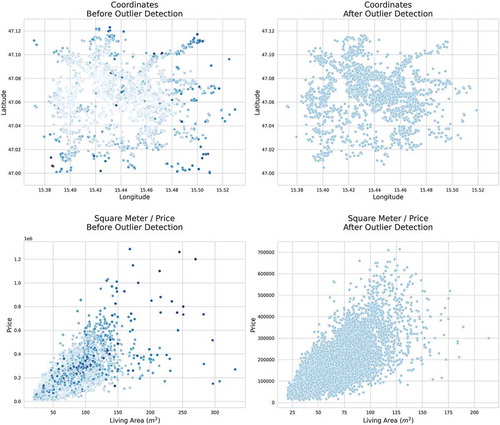
Table 8 shows a summary of the data before and after the cleaning.

Table 8. Different stages of the data cleaning process

	Raw data	After excluding missing price and $m$^2	After cleaning
Median Price	159,500	160,708	160,000
Mean Price	181,703	181,240	175,435
Count	18,957	11,250	10,797

4.4. Variable creation and transformation

ML algorithms perform better with more observations and more input variables per observation. We therefore construct a variety of variables from the existing dataset variables as well as additional data sources. For example, for each apartment we calculate the distance to the city centre and to the nearest school, and we establish yearly, quarterly, and monthly time variables from the dates of sale. To better describe neighbourhood effects, we establish new variables based on location clustering (we use a k-Means unsupervised learning algorithm for this step). Additionally, we include data on the noise level of nearby streets. For a summary of the individual characteristics, see Table A3 and A4 in Appendix C.

We transform price into log price to make the target variable more normal. This is a standard technique to improve the overall performance of house-price prediction models. To re-transform the estimated log values at the end, we apply the smearing adjustment factor introduced by Duan (1983). This adjusts the estimated price ${\hat{p}}_{\hspace{0.17em}}$ such that:

(7) $E\left[\hat{p}\right]=\hat{\phi }\mathrm{e}\mathrm{x}\mathrm{p}\left(X\hat{\beta }\right)=\hat{\phi }\mathrm{e}\mathrm{x}\mathrm{p}\left[\mathrm{l}\mathrm{n}\left(\hat{p}\right)\right]$(7)

$with\hat{\phi }=\frac{1}{n}\sum _N^{n=1}exp({\epsilon }_i)$

where X is a vector of property i specific characteristics, $\hat{\beta }$ is a vector containing the corresponding characteristic shadow prices, and $\mathrm{l}\mathrm{n}\left(\hat{p}\right)$ is the predicted log price obtained from the ML model. N is the sample size, i the difference between observed and predicted values in log form (i.e. $ln\left(p_i\right)-ln({\hat{p}}_i$)), and $\hat{\phi }$ the adjustment factor.^{14 15}

Furthermore, we centre and scale all numeric variables to lie between 0 and 1. Scaling inputs helps to avoid situations where one or several features dominate others in magnitude and as a result the model hardly picks up the contribution of the smaller scale variables, even if they are strong. Some ML algorithms are more sensitive to this than others.¹⁶

4.5. Train-test split

To evaluate the different metrics, we use a growing window 5-fold cross validation as depicted in Figure 2. Since, the aim of an AVM is to perform well on new unseen data, we use a growing window approach to judge each algorithm on future data (see e.g. Cerqueira et al., 2019). For each fold, the training data are used to find the best set of parameters (using cross validation) and then the metric is calculated by using the test set. The final error is then computed by the average over all 5 prediction sets according to each metric.

Figure 2. 1-step ahead train/test split

4.6. Model tuning and selection

We train the following prediction methods: Linear Regression (hedonic) model (M1), Random Forest model (M2), Multivariate Adaptive Regression Splines (MARS) model (M3), a model that uses Quantile Regression with LASSO penalties (M4), and a Neural Net model (M5).

We chose these methods because they are widely applied in the AVM literature and of similar predictive power. A short description of each of these methods can be found in Appendix A. We use ‘R’ (R Core Team, 2012) to perform all computations.¹⁷

Most of the models we consider need some degree of model tuning to find the optimal hyperparameters. This involves making comparisons between different model versions. We use grid-searches on hyper-parameters and 10-fold cross-validation on the training set to select between model variations of one model family.¹⁸

We use the RMSE metric to measure performance in the tuning stage. This raises an important point: Performance metrics are needed at two stages in the modelling process. First, they are needed to tune the individual ML methods. Second, they are used to compare performance across different ML methods. While we focus here on the use of metrics in the second stage, similar issues arise in the first stage. Here it is practical for us to focus on a single metric during the first stage, so as to obtain unambiguous results when tuning the model. One attraction of RMSE in this regard is that it is a standard tuning metric which can often be taken ‘off-the-shelf’ in ML estimation packages. If it is applied to the prices in log form then it corresponds to our LRMSE metric (which satisfies symmetry).¹⁹ The result of this exercise is the model specification that then gets evaluated in the final stage via the test set (hold-out sample).

We use the metrics described above to compare the performance of five ML prediction methods. Performance across methods is then evaluated using the holdout sample. We use all 48 metrics discussed above to make this evaluation, and compare how sensitive the results are to the choice of metric.

5. Metric results and implications

5.1. The sensitivity of rankings to the choice of performance metric

Each apartment $i$ in the test set is characterised by a price $\left(p_i\right)$ and a set of characteristics $X_i=x_{i,1},x_{i,2},\dots ,x_{i,d}$, where $x_{i,j}$ denotes the $j$th characteristic of the $i$th apartment. Each of the trained models (M1 to M5) is provided with the set $X_i$and generates predictions for the logarithm of the price $ln\left(p_i\right)$ for each apartment.$i$.

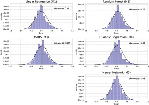
Figure 3 illustrates the distribution of the log errors for each model.²⁰ The black solid line corresponds to the normally distributed error density derived from the mean and standard deviation of the observed errors. The skewness scores indicate how skewed a distribution is (a skewness score of zero represents a symmetric distribution). All our models have moderate positive skewness scores, implying they have larger overpredictions than underpredictions (in log-difference form). The Random Forest model (M2) is least affected by skewness.

Figure 3. Error distribution of model M1 – M5

All metrics discussed in this paper are calculated using the set of true prices ($p_i$) and the set of predicted prices (${\hat{p}}_i$); Table A2 lists the output for all 48 metrics.

In addition to these average cross-validation results, we also present the best model for each individual fold in Table A2. Table A2 illustrates that the overall performance is stable across the different sub-datasets. M2 (Random Forest) performs best for 30 metrics, M3 (Multivariate Adaptive Spline Model) is best for 10 metrics, M4 (Quantile Regression with LASSO Penalty) is best for 5 metrics, M5 (Neural Net) is best for 2 metrics, and M1 (Linear Regression) is best for 1 metric.

An important additional consideration to the overall number of ‘wins’ by individual models is the pattern that emerges. While M2 (Random Forest) dominates overall, it does not do so for metrics in the Mean Bias class or the Squared-Ratio class. For these classes M3 (Multivariate Adaptive Spline Model) outperforms M2 (Random Forest).

5.2. What set of metrics do we recommend?

It is not always practicable to calculate the performance of alternative models for nearly 50 metrics. Hence there is a need to prioritise and decide which metrics are most important.

Table 9 lists some of the most commonly used metrics in the AVM literature: Mean Prediction Error (MPE), Mean Absolute Prediction Error (MAPE), Coefficient of Dispersion (COD), Root Mean Squared Error (RMSE), Mean Absolute Error (MAE), and $R^2$. Using these metrics, the model of choice is M2 (Random Forest) for all these metrics except MPE (where model M4 performs best).

Table 9. Model performance rankings based on metrics from the AVM literature

Class	Metric	M1	M2	M3	M4	M5
Average Bias	MPE	0.059	−0.029	0.023	0.017	0.043
Absolute Difference	MAE/10,000	4.011	3.624	3.732	3.763	3.948
Absolute Ratio	MAPE	0.228	0.195	0.210	0.208	0.227
Absolute Ratio	COD	0.212	0.198	0.208	0.205	0.223
Squared Difference	RMSE/10,000	6.119	5.214	5.284	5.463	5.742
Squared Difference	1-R^2	0.448	0.321	0.330	0.354	0.391

The prediction methods are as follows: M1 = Linear Regression; M2 = Random Forest; M3 = Multivariate Adaptive Regression Spline; M4 = Quantile Regression with Lasso Penalty; M5 = Neural Network

The displayed metric values are the average values over 5 folds on the testing sets.

In Table 10 we present seven metrics (one for each class) that we believe provide a better basis for evaluating AVM performance. It is important to select a mix of metrics that capture different aspects of model performance.

Table 10. Predictive performance of methods M1-M5 (Short List)

Class	Metric	M1	M2	M3	M4	M5
Average Bias	LMDPE	0.048	−0.041	0.007	0.009	0.008
Absolute Difference	MAE/10,000	4.011	3.624	3.732	3.763	3.948
Absolute Ratio	mmMAPE	0.288	0.269	0.270	0.273	0.284
Squared Ratio	LRMSE	0.309	0.298	0.294	0.300	0.306
Squared Difference	RMSE/10,000	6.119	5.214	5.284	5.463	5.742
Percentage Ratio	mmPER(10)	0.697	0.658	0.686	0.671	0.703
Quantile	IQRat	0.322	0.297	0.327	0.305	0.330

The displayed metric values are the average values over 5 folds on the testing sets.

LMDPE is selected as a measure of central tendency (bias) in preference to MPE in Table 8 since it is symmetric in bias and more robust to outliers. The greater robustness follows from LMDPE being median based.

MAE, mmMAPE, LRMSE, RMSE, mmPER and IQRAT all measure dispersion. Both MAE and RMSE satisfy symmetry-in-dispersion and we keep them to represent the absolute-difference and the squared-difference metrics. Both of these metrics are also widely available in statistical packages. Note that as an absolute-difference metric MAE is more robust to outliers than RMSE. Thus, depending on the dataset and/or task at hand, one would give one or the other more weight.

The two absolute-ratio metrics in Table 9, MAPE and COD, do not satisfy symmetry-in-dispersion. We replace them with mmMAPE, which is a symmetrified version of a number of different widely used metrics, of which MAPE is just one example.²¹

The squared-ratio metrics, range metrics, and quantile metrics were not represented in Table 9. We choose LRMSE as the representative for the squared ratio class. It satisfies symmetry in-dispersion and is also easily calculated with most statistical packages (by simply applying RMSE to the log prices).

Our representative for the range metrics is mmPER(10), while IQRat is chosen as the representative for the quantile metrics. The results for these metrics are shown in Table 10. The metrics LMDPE, mmPER and IQRAT are new to the literature.

In Table 10, M2 (Random Forest) performs best according to MAE, mmPER(10) and IQRAT, while M3 (Multivariate Adaptive Regression Spline) performs best according to MDPE, and LRMSE. For LMDPE, the difference in the results between M3, M4 and M5 is very small. All three medians are closely centred on the target value of zero. Similarly, the difference in performance for LRMSE between M3 and M2 is minimal. Hence based on this short list, M2 performs best in terms of average dispersion, although it has a slight tendency to overpredict the median error ratio.

6. Conclusion

The choice of performance metric to compare alternative ML models is a potential source of confusion in the AVM literature. A number of metrics are used, but there has been little attempt to undertake a systematic analysis of their properties. We collect 48 different metrics and structure them according to their mathematical formulation into seven classes. These are: the class of bias metrics, two ways of constructing difference metrics (absolute and squared differences), two ways of constructing ratio metrics (absolute and squared ratios), metrics based on percentage-ranges, and quantile-based metrics. This systematic review and classification of existing metrics is one of the contributions in this paper.

Users will find metrics from one or the other class more appropriate depending on how they want to treat errors. However, not all metrics of a class are equally well suited as performance metrics for AVMs. For example, some very popular metrics do not treat prediction errors in a symmetric manner. We differentiate between two types of symmetry that are important in this context: symmetry-in-bias (important for average-bias metrics) and symmetry-in-dispersion (important for the other classes). Failure to satisfy these symmetry criteria implies some arbitrariness in the metric formula. For example, it can lead to asymmetric treatment of the left and right tails of the error distribution. Such asymmetries can distort results in unexpected ways, potentially producing a misleading ranking of ML methods.

Another contribution of this paper is the transformation of some commonly used metrics that violate the symmetry conditions. In this way, we introduce a number of new metrics into the literature. These new metrics still measure the same type of error as before, but do this now in a symmetric way.

Our empirical applications illustrate the need to think carefully about which set of metrics should be used to choose between models. We evaluate five ML models with 48 different metrics and find that each model performs best at least once (depending on the chosen metric). Thus, arbitrarily choosing a metric can lead to an inappropriate model being chosen. We provide some guidance in this matter by presenting a shortlist of seven metrics – one for each class. Each of these metrics addresses a different aspect of the performance evaluation problem; taken together, this shortlist will provide a good overall evaluation of alternative AVM models. Similarly, if a user is mainly interested in one class of errors, the shortlist provides an ideal candidate.

The following three ingredients are necessary to build effective ML prediction models according to Kuhn (2016):

(1) intuition and deep knowledge of the problem context,

(2) relevant data, and

(3) a versatile computational toolbox of algorithms.

We recommend adding another ingredient to this list:

(4) the appropriate choice of performance metrics for model selection via cross-validation.

Acknowledgments

We acknowledge financial support for this project from the Austrian Research Promotion Agency (FFG), grant #10991131.

We also thank ZTdatenforum (www.zt.co.at) for providing us with the dataset.

Disclosure statement

No potential conflict of interest was reported by the authors.

Additional information

Funding

This work was supported by the Österreichische Forschungsförderungsgesellschaft FFG [grant #10991131].

Notes on contributors

Miriam Steurer

Miriam Steurer is an economist at the Institute of Economics at University of Graz, Austria. She obtained her PhD from University of New South Wales in Australia in 2008. Her current research focuses mainly on the application of machine learning methods to the real estate market. As part of this research agenda, she is developing Automated Valuation Models for the Austrian real estate market in partnership with the firm ZTdatenforum. This project is funded by the Austrian Research Promotion Agency (FFG). Dr Steurer is included in the expert roster of the IMF Statistical Department and was part of the Technical Advisory Group to the 2017 International Comparison Program of the World Bank.

Robert J. Hill

Robert J. Hill is Professor of Macroeconomics at University of Graz, Austria. Before that he was Professor of Economics at University of New South Wales in Australia. He obtained his PhD in Economics in 1995 from University of British Columbia in Canada. He is a Fellow of the Academy of the Social Sciences of Australia, the Society for Economic Measurement, and a member of the Conference on Research in Income and Wealth at the NBER. He is currently serving on World Bank and UN task forces. He has previously served on task forces for the UK Statistical Authority and Eurostat. From 2008 to 2014 he was Managing Editor of the Review of Income and Wealth. He has published widely in journals such as American Economic Review, International Economic Review, Review of Economics and Statistics, Journal of Econometrics, Journal of Business and Economic Statistics, Economic Inquiry, Regional Science and Urban Economics, Journal of Housing Economics, and Journal of Real Estate Finance and Economics.

Norbert Pfeifer

Norbert Pfeifer is a PhD student in the Institute of Economics at University of Graz; Austria (supervisor: Prof. Hill). In 2019 he presented papers at both the American Real Estate and Urban Economics Association (AREUEA) conference at Bocconi University in Milan, and at the European Real Estate Society (ERES conference at Cergy-Pontoise in France. His main research area lies in the application of computer vision and natural language processing applied to the field of housing. He is also engaged in the construction of an Automated Valuation Model for the Austrian real estate sector.

Notes

1. This point has been stressed both in the academic literature (see Varian, 2014) as well as in practical applications (e.g. the winning entries of Kaggle competitions (www.kaggle.com/competitions) almost invariably use ML methods).

2. Sometimes the term ‘Mass Appraisal’ is used instead of AVM in the literature.

3. A discussion on these 5 algorithms can be found in Appendix B.

4. For example, none of the AVM providers in Austria publish information on their algorithms, their objective functions, or performance metrics.

5. Some of the metrics themselves can be derived from loss functions.

6. Although in two of the models (models M3 and M4) we added penalisation terms to the loss function to allow for variable selection and to minimise over-fitting of the ML model.

7. We were told that this is the approach followed by banks in Austria.

8. Underpinning this class is the absolute loss function: $L1=|p-\hat{p}$|.

9. Underpinning this class is the squared loss function: $L2={\left(p-\hat{p}\right)}^2$

10. Either in absolute or squared terms.

11. It is worth noting that $\frac{p_n}{{\hat{p}}_n}$−1 is a first order Taylor series approximation of $ln\left(p_n/{\hat{p}}_n\right)$

12. PER measures the expected loss for a $1-0$ loss function, where L = 1 if the ratio error is greater than x, and L = 0 otherwise.

13. Alternatively, we could have imputed the missing characteristics based on their statistical attributes (such as mean, or median values) or by using more sophisticated methods (e.g. missing forest or k-nearest-neighbours algorithms).

14. This Jensen-type correction is needed because $E[\hat{p}]=E[\mathrm{e}\mathrm{x}\mathrm{p}(X\hat{\beta }+ϵ)]\ne \mathrm{e}\mathrm{x}\mathrm{p}(X\hat{\beta })$.

15. Given that we are training the random forest model on actual prices rather than log prices (no adjustment is needed) and the applied neural network with one hidden layer relies on a linear relationship between the predicted price and the observed inputs – as for the remaining methods – equation (7)(7) $E\left[\hat{p}\right]=\hat{\phi }\mathrm{e}\mathrm{x}\mathrm{p}\left(X\hat{\beta }\right)=\hat{\phi }\mathrm{e}\mathrm{x}\mathrm{p}\left[\mathrm{l}\mathrm{n}\left(\hat{p}\right)\right]$(7) can be used for the re-transformation adjustment without any further assumption.

16. In particular neural network algorithms do not have the property of scale invariance (see e.g. Hastie et al., 2009).

17. There are various packages in ‘R’ that can be used to train ML algorithms. For many ML related processes, the ‘caret package’ (Kuhn, 2008) is a starting point as it provides many different ML techniques in one comprehensive framework.

18. Note, we completely retrain all models after each new train-test split.

19. When LRMSE is used to tune the models in the first stage, then to ensure internal consistency LRMSE should also be one of the metrics used to compare performance across ML methods in the second stage.

20. We take the log errors from fold 5 to construct the histograms in Figure 3.

21. Note that LMAPE or DM1 could also play this role.

22. For a survey of this literature see Hill (2013).

23. See Diewert (2003) and Malpezzi (2008) for a discussion of some of the advantages of the semilog functional form in a hedonic context.

24. We follow Hastie et al. (2009) and first create linear basis functions with a ‘knot’ at each observed input value $x_{i,j}$, such that for each $x_{i,j}$ we have a function-pair of the form$:max\left(0,X_j-x_{i,j}\right)$ and $max\left(0,x_{i,j}-X_j\right)$ (Hastie et al., 2009). These piece-wise linear basis functions can then be transformed by multiplying them together (which can form non-linear functions).

25. By adding the L1 penalty term to the Error term, the LASSO exploits the bias-variance trade-off to produce models that increase the bias in the model in order to greatly reduce the model variance and thereby combat the problem of collinearity (Kuhn, 2016).

26. Note that for each quantile $\tau$ the solution to the minimisation problem yields a separate set of regression coefficients.

27. Sherwood (2017) provides an R-package called ‘rqPen’ which implements (12).

28. The error rate is defined as the difference between the Neural Net prediction and the observed transaction price.

Appendix A.

Results

Table A1. Predictive performance of methods M1-M5 (Full-List)

		Model
Class	Metric	M1	M2	M3	M4	M5
Average Bias	MBE/1000	8.192	−1.384	2.560	2.210	4.588
	MDBE/1000	7.188	−7.067	0.714	1.501	1.115
	MPE	0.059	−0.029	0.023	0.017	0.043
	MPE’	−0.042	−0.124	−0.068	−0.078	−0.056
	MDPE	0.049	−0.040	0.007	0.009	0.009
	LMDPE	0.048	−0.041	0.007	0.009	0.008
	100 x LMPE	1.328	−6.847	−1.737	−2.377	−0.280
Absolute Difference	MAE/10,000	4.011	3.624	3.732	3.763	3.948
	MDAE/10,000	2.725	2.532	2.673	2.494	2.672
Squared Difference	RMSE/10,000	6.119	5.214	5.284	5.463	5.742
	1-R2	0.448	0.321	0.330	0.354	0.391
	1-CC	0.234	0.163	0.179	0.195	0.213
	NRMSE	0.095	0.082	0.083	0.085	0.090
	SNR	0.528	0.644	0.447	0.494	0.528
	SDE/10,000	6.054	5.194	5.279	5.460	5.715
Absolute Ratio	MAPE	0.228	0.195	0.210	0.208	0.227
	MAPE’	0.248	0.248	0.239	0.244	0.242
	MDAPE	0.177	0.153	0.164	0.155	0.166
	sMAPE	0.111	0.103	0.105	0.105	0.110
	sMDAPE	0.085	0.077	0.082	0.077	0.084
	COD	0.212	0.198	0.208	0.205	0.223
	COD’	0.255	0.233	0.240	0.245	0.242
	LMAPE	0.227	0.210	0.215	0.215	0.224
	mmMAPE	0.288	0.269	0.270	0.273	0.284
	DM1	0.101	0.095	0.091	0.095	0.098
Squared Ratio	MSPE	0.092	0.068	0.077	0.077	0.100
	MSPE’	0.181	0.206	0.167	0.183	0.163
	LSDE	0.308	0.289	0.294	0.299	0.305
	LRMSE	0.309	0.298	0.294	0.300	0.306
	LMSPE	0.096	0.089	0.087	0.090	0.094
	mmMSPE	0.218	0.223	0.193	0.208	0.208
	DM2	0.273	0.274	0.244	0.260	0.262
Percentage Ratio	PER(10)	0.686	0.645	0.670	0.654	0.689
	PER(20)	0.446	0.375	0.422	0.402	0.424
	PER(30)	0.281	0.206	0.250	0.246	0.255
	PER’(10)	0.680	0.646	0.669	0.651	0.685
	PER’(20)	0.422	0.398	0.403	0.391	0.418
	PER’(30)	0.238	0.232	0.230	0.228	0.246
	LPER(10)	0.682	0.646	0.670	0.654	0.689
	LPER(20)	0.440	0.391	0.414	0.398	0.424
	LPER(30)	0.271	0.222	0.240	0.242	0.256
	mmPER(10)	0.697	0.658	0.686	0.671	0.703
	mmPER(20)	0.476	0.434	0.459	0.436	0.463
	mmPER(30)	0.322	0.272	0.301	0.293	0.312
Other	IQRat	0.322	0.297	0.327	0.305	0.330
	9010IQRat	0.717	0.630	0.680	0.709	0.694
	IQLev/10,000	5.202	4.792	5.304	4.907	5.205
	9010IQLev/100,000	1.191	1.097	1.183	1.190	1.254

The displayed metric values are the average values over 5 folds on the testing sets.

Table A2. Cross validation results

Metric	Fold-1	Fold-2	Fold-3	Fold-4	Fold-5
MBE/1000	M4	M3	M3	M5	M3
MDBE/1000	M5	M2	M5	M3	M5
MPE	M4	M2	M4	M4	M3
MPE’	M3	M1	M1	M1	M1
MDPE	M5	M2	M5	M3	M5
MAE/10,000	M2	M2	M2	M4	M2
MDAE/10,000	M2	M2	M4	M4	M4
RMSE/10,000	M3	M2	M2	M4	M2
1-R2	M3	M2	M2	M4	M2
1-CC	M2	M2	M2	M2	M2
NRMSE	M3	M2	M2	M4	M2
SNR	M3	M3	M3	M3	M5
SDE/10,000	M3	M2	M2	M4	M2
MAPE	M2	M2	M2	M2	M2
MAPE’	M3	M2	M5	M4	M5
MDAPE	M2	M2	M4	M4	M4
sMAPE	M2	M2	M2	M4	M5
sMDAPE	M2	M2	M4	M4	M4
COD	M2	M2	M2	M4	M2
COD’	M2	M2	M2	M2	M2
LMAPE	M2	M2	M2	M4	M5
mmMAPE	M3	M2	M2	M4	M5
DM1	M3	M2	M3	M4	M5
MSPE	M2	M2	M2	M2	M2
MSPE’	M3	M5	M5	M3	M4
LSDE	M3	M2	M2	M2	M2
LRMSE	M3	M2	M3	M4	M5
LMSPE	M3	M2	M3	M4	M5
mmMSPE	M3	M3	M5	M3	M4
DM2	M3	M3	M5	M3	M4
PER(10)	M2	M2	M2	M4	M4
PER(20)	M2	M2	M2	M2	M4
PER(30)	M2	M2	M2	M2	M2
PER’(10)	M2	M2	M4	M4	M4
PER’(20)	M2	M2	M4	M4	M5
PER’(30)	M3	M3	M2	M4	M4
LPER(10)	M2	M2	M4	M4	M4
LPER(20)	M2	M2	M2	M4	M4
LPER(30)	M2	M2	M2	M4	M2
mmPER(10)	M2	M2	M2	M4	M1
mmPER(20)	M2	M2	M4	M4	M4
mmPER(30)	M2	M2	M2	M4	M4
IQRat	M2	M2	M4	M4	M4
9010IQRat	M2	M2	M2	M2	M2
IQLev/10,000	M2	M2	M4	M2	M2
9010IQLev/100,000	M2	M2	M2	M2	M4

Only the best performing model for each fold and each metric is reported.

Appendix B.

Description of the applied models

Model M1: Linear Regression

The Linear Regression model (hedonic model) serves as a benchmark for the ML models. Hedonic models have originally been used in economics to model the prices for products subject to rapid technological change, such as cars and computers (see for example, Grilliches, 1961). They have since become the standard model for house price regressions, especially when it comes to house price indices.²² The hedonic model regresses the price of a product on a vector of characteristics, whose prices are not independently observed, thereby generating shadow prices for these characteristics. If the logarithm of the price is used on the left hand side, the interpretation changes slightly: instead of shadow prices on characteristics, the estimated parameters then estimate the percentage influence of these characteristics.²³ Here we regress the logarithm of price on a linear function of explanatory characteristics. All categorical variables are included as dummy variables.

Thus, the model parameters (the βs) are chosen to minimise the Sum-of-Squared Errors (SSE):

$\underset{\beta }{min}\sum _i^N(y_i-\left({\beta }_0+\beta x_i\right){)}^2,$

where ${\beta }_0$ indicates the intersect term.

Model M2: Random Forest

The random forest technique was first proposed by Breiman (2001) and has since become one of the most popular ML methods. For house price predictions they have first been used by Antipov and Pokryshevskaya (2012).

Random Forests are tree-based non-parametric ensemble methods with uncorrelated decision trees as base learners. Each tree is a simple model that is built independently using a random sample of the available variables. Averaging over many independently built trees reduces variance, increases robustness, and makes the method less prone to over-fitting. Different techniques exist to construct base learners (the individual trees). The most common one is the ‘Classification And Regression Tree’ (CART) method, also known as the recursive partitioning procedure which was proposed by Breiman et al. (1984).

Building a CART tree begins by splitting the dataset S into two groups (S1 and S2) so that the overall sum of squared errors (SSE) are minimised. To find the predictor and split value that minimises the SSE, it tries out every distinct value (split point s) of every predictor (Kuhn, 2016). Thus, for each variable j and each split point s, we minimise the following:

$\underset{j,s}{min}\left(\sum _{i\epsilon S_1}(y_i-{\bar{y}}_1{)}^2+\sum _{i\epsilon S_2}(y_i-{\bar{y}}_2{)}^2\right),$

where (${\bar{y}}_1$) and (${\bar{y}}_2$) denote the averages of the target values of $S_1$ and $S_2$ respectively. This process is then repeated within each subgroup, continuously splitting the data into smaller subsets.

A random forest builds an ensemble out of many such trees. Correlation between predictors is reduced by providing the algorithm with a randomly chosen number of predictors at each split (rather than the full set of available predictors). The number of predictors presented to the algorithm at each step is generally referred to as ‘mtry’ and is the main tuning parameter of the random forest model. The other tuning parameter is the number of individual trees that are grown and averaged. We use grid searches over these tuning parameters and CV using the LRMSE metric to find the best performing version of the random forest model at this stage.

Random Forests are robust to outliers and a good method when data are noisy. A Random Forest model can consist of mixed variables (numerical and categorical), and/or contain missing values. These features – plus the fact that they are relatively easy to implement – have made Random Forest models very popular.

Model M3: Multivariate Adaptive Regression Splines (MARS)

An example of a non-parametric extension of linear regression is the multivariate adaptive regression spline (MARS), which was introduced by Friedman (1991). The basic idea is as follows: ‘A piecewise polynomial function $f\left(x\right)$ is obtained by dividing the domain of $X$ into continuous intervals and representing $f$ by a separate polynomial in each interval.’ (Hastie et al., 2009). Continuity constraints are introduced to make the resulting polynomial function $f\left(x\right)$ continuous at the threshold points (knots). The ‘division’ of the domain $X$ is done via hinge functions – linear basis functions that identify the threshold points (knots), where a linear regression model is shifted into a different regression line. The first step in the MARS algorithm is thus the formation of these hinge functions.²⁴

Following the terminology in Hastie et al. (2009), we can write the regression problem as follows:

$f\left(X\right)={\beta }_0+\sum _{m=1}^M{\beta }_m{h}_m\left(X\right),$

where each $h_m\left(X\right)$ represents a hinge function or a product of hinge functions.

The model building process of MARS is then like a stepwise linear regression using the basis functions – and their transformations – as inputs (Hastie et al., 2009).

The model coming out of this regression will be over-fitted and therefore needs to be trimmed back. This can be done via a stepwise term deletion procedure. One by one the terms, that are least helpful in reducing the overall error, are removed until only the intercept term remains. Each of these deletions leaves us with a possible model. We again use CV with LRMSE as the metric to select the one that fits our data best.

Regression splines provide a highly versatile regression technique that is relatively easy to implement and has many benefits: it automatically performs variable selection, variable transformation, and interaction detection. It also generally produces lower errors than linear regression techniques. Like linear regression, MARS is relatively easy to interpret, but is – because of the non-parametric parts – more flexible. Due to these benefits, applications of MARS are diverse and range from forecasting grid power output (Li et al., 2016) to droughts in Australia (Deo et al., 2017).

Model M4: Quantile Regression with LASSO Penalty

First introduced by Koenker and Bassett (1978), Quantile Regression (QR) explicitly addresses a weakness of standard regression techniques: the focus on predicting in the vicinity of the mean of the distribution, and hence often poor performance away from the mean (Zou, 2006). LASSO penalties were introduced by Tibshirani (1996) as a method to perform parameter shrinkage and parameter selection in linear regression models, but can also be applied to other statistical models. LASSO stands for ‘Least Absolute Shrinkage and Selection Operator’ and refers to a penalty in L1 norm of the coefficient vector. It is particularly well suited to problems with sparse data (Hastie et al. (2009)).²⁵

The combination of Quantile Regression with L1 norm shrinkage was first applied by Koenker (2004). Wu and Liu (2009) show that the inclusion of a LASSO penalty parameter can improve interpretability without losing accuracy in fit. He et al. (2016) apply a Quantile regression model with LASSO penalties to identify genetic features that influence quantitative traits. We are not aware of any applications in the housing market of this method thus far.

Unlike least-squares regression, where the coefficients are estimated by solving the least squares minimisation problem, the coefficients in a linear quantile regression are chosen by minimising the sum of asymmetrically weighted absolute errors:

$\underset{{\beta }_{\tau }}{min}\sum _{i=1}^N{\rho }_{\tau }\left(y_i-x_i^T{\beta }_{\tau }\right),$

where τ refers to the individual quantile being modelled, and the weights $\rho \tau \left(u\right)$ are given by: $\rho \tau \left(u\right)=\tau u\mathrm{i}\mathrm{f}u>0,\mathrm{a}\mathrm{n}\mathrm{d}-\left(1-\tau \right)u$ otherwise.²⁶

After adding the LASSO penalty term, (11) becomes:

$\underset{{\beta }_{\tau }}{min}\sum _{i=1}^N{\rho }_{\tau }\left(y_i-x_i^T{\beta }_{\tau }\right)+\alpha \sum _{j=1}^d\left|{\beta }_{\tau ,j}\right|.$

Tuning of the model is done by choosing the number of quantiles τ and the regularisation parameter $\alpha$, which controls the strength of the shrinkage process (and thus also variable selection). Too much shrinking leaves a sub-optimal model, while too little shrinking tends to lead to poor interpretability (and over-fitting). Again, for model selection in the tuning phase, we use the LRMSE metric and cross-validation to choose the best-performing regularisation parameter.²⁷

Model M5: Neural Nets

Neural Net models have a wide variety of applications, most notably in speech recognition and machine translation, computer vision (object and activity recognition), and robotics (e.g. self-driving cars). They are particularly useful when automated feature selection is needed and when the dataset is large. Our dataset, consisting of just under 6000 transactions and a limited number of variables, is rather small for a Neural Net application. Neural net applications to the estimation of house prices include Selim (2009), Peterson and Flanagan (2009), Zurada et al. (2011), Ahn et al. (2012), Yacim and Boshoff (2018), and Hastie et al. (2009) describe the basic idea behind Neural Nets as extracting ‘linear combinations of the inputs as derived features, and then modelling the target as a nonlinear function of these features’. The most basic structure of Neural Nets consists of an input layer, one or more hidden layers, and an output layer. Functions of increasing complexity can be modelled by adding more layers and more units within a layer (Goodfellow et al., 2016). The strength of individual connections is indicated by weights. Hidden layers find features within the data and allow the following layers to operate directly on those features rather than the entire dataset. By repeatedly adjusting the weights – the strength of individual connections between units – the error rate is minimised.²⁸ Thus, a Neural Net aims to minimise the errors, where the errors are considered to be a function of the weights of the network (generally the sum of squared errors or cross-entropy). However, as the global minimum of the error function would likely lead to an overfitted solution, some regularisation – either stopping early or a penalty term – is needed. The penalty term is generally implemented via ‘weight decay’, which is a penalty in L2 norm (Hastie et al., 2009).

Here, we implement a simple feed-forwards Neural Net model via the ‘nnet-package’ in R (Ripley, 2016). This package fits a single hidden-layer Neural Network with two tuning parameters: the number of units in the hidden layer and weight decay (to avoid over-fitting). We calibrate the model via repeated grid searches on combinations of the tuning parameters.

Appendix C.

Description of data

Table C1. Mean values of characteristics in training sets

Fold	1	2	3	4	5	Mean
Price	169,266.30	169,799.26	171,277.46	172,186.19	174,081.00	171,322.04
Living Area	66.85	66.75	66.88	66.85	66.87	66.84
Living Area squared	5001.04	4977.40	4999.06	4998.18	5000.19	4995.17
Latitude	47.07	47.07	47.07	47.07	47.07	47.07
Longitude	15.44	15.44	15.44	15.44	15.44	15.44
Distance to centre	2.71	2.75	2.76	2.76	2.77	2.75
Month	6.67	6.32	6.61	6.40	6.43	6.49
Year	2016.62	2016.85	2017.07	2017.28	2017.50	2017.06
Balcony	0.27	0.26	0.25	0.25	0.25	0.26
Parking	0.09	0.10	0.09	0.10	0.11	0.10
Outside Space	0.20	0.20	0.20	0.20	0.19	0.20
New Building	0.46	0.46	0.46	0.45	0.45	0.46
Age Category	1.81	1.86	1.91	1.96	1.96	1.90
Distance to School	387.76	391.80	395.24	397.35	398.43	394.12
Street Noise	61.18	60.66	60.74	60.91	60.91	60.88
Zoning* (mode)	1	1	1	1	1	1
Cluster (mode)	0	0	0	0	0	0
Count	6298.00	7198.00	8098.00	8997.00	9897.00	8097.60

*Zoning categories: 1 = Residential area, 2 = Core area, 3 = Industrial area, 4 = Building land, 5 = Mixed area

Table C2. Mean values of characteristics in testing sets

Fold	1	2	3	4	5	Mean
Price	173,528.81	183,099.73	180,571.43	193,022.80	190,333.21	184,111.20
Living Area	66.04	67.93	66.65	67.06	66.22	66.78
Living Area squared	4812.01	5172.30	4993.76	5020.29	4931.03	4985.88
Latitude	47.06	47.07	47.06	47.06	47.06	47.06
Longitude	15.44	15.44	15.44	15.44	15.43	15.44
Distance to centre	3.01	2.81	2.80	2.83	2.89	2.87
Month	3.89	8.88	4.51	6.80	7.53	6.32
Year	2018.40	2018.84	2019.24	2019.65	2020.11	2019.25
Balcony	0.20	0.19	0.18	0.24	0.29	0.22
Parking	0.10	0.09	0.10	0.20	0.15	0.13
Outside Space	0.20	0.18	0.17	0.18	0.15	0.18
New Building	0.47	0.41	0.42	0.37	0.37	0.41
Age Category	2.18	2.29	2.46	1.96	1.44	2.07
Distance to School	420.05	422.74	416.45	409.29	424.67	418.64
Street Noise	56.98	61.38	62.48	60.93	62.73	60.90
Zoning* (mode)	1	1	1	1	1	1
Regional cluster (mode)	9	9	0	0	0	0
Count	900.00	900.00	900.00	900.00	900.00	900.00

*Zoning categories: 1 = Residential area, 2 = Core area, 3 = Industrial area, 4 = Building land, 5 = Mixed area

References

- Abdul-Wahab, S. A., & Al-Alawi, S. M. (2002). Assessment and prediction oftropospheric ozone concentration levels using artificial neural networks. EnvironmentalModelling and Software, 17(3), 219–228. https://doi.org/10.1016/S1364-8152(01)00077-9
- Agarwal, S., Ambrose, B. W., & Yao, V. (2020). Can regulation de-bias appraisers? Journal of Financial Intermediation, 44, 100827. https://doi.org/10.1016/S1364-8152(01)00077-9
- Ahn, J. J., Byun, H. W., Oh, K. J., & Kim, T. Y. (2012). Using ridge regression with genetic algorithm to enhance real estate appraisal forecasting. Expert Systems and Applications, 39(9), 8369–8379. https://doi.org/10.1016/j.eswa.2012.01.183
- Akaike, H. (1973). Information theory and an extension of the maximum likelihood principle. In B. N. Petrov & F. Csáki (Eds.), 2nd international symposium on information theory (pp. 267–281). Tsahkadsor, Armenia, USSR, September 2–8, 1973 Akadémiai Kiadó. Republished in Kotz, S.; Johnson, N. L., eds. (1992), Breakthroughs in Statistics, I, SpringerVerlag, pp. 610–624. Originally published in Proceeding of the second international symposium on information theory(pp. 267–281) (B. N. Petrovand & F. Caski, eds.). Budapest: Akademiai Kiado, 1973.
- Antipov, E., & Pokryshevskaya, E. B. (2012). Mass appraisal of residential apartments: An application of random forest for valuation and a CART-based approach for model diagnostics. Expert Systems with Applications, 39(2), 1772–1778. https://doi.org/10.1016/j.eswa.2011.08.077
- Bajari, P., Nekipelov, D., Ryan, S. P., & Yang, M. Machine learning methods for demand estimation. (2015, May). American Economic Review, 105(5), 481–485. https://doi.org/10.1257/aer.p20151021
- Bogin, A. N., & Shui, J. (2018). Appraisal accuracy, automated valuation models, and credit modeling in rural areas. In FHFA staff working papers 18–03. Washington, DC: Federal Housing Finance Agency.
- Breiman, L. (2001). Random forests. Machine Learning, 45(1), 5–32. https://doi.org/10.1023/A:1010933404324
- Breiman, L., Friedman, J., Stone, C. J., & Olshenand, R. A. (1984). Classification and regression trees. Taylor & Francis.
- Ceh, M., Kilibarda, M., Lisec, A., & Bajat, B. (2018). Estimating the performance of random forest versus multiple regression for predicting prices of the apartments. ISPRS International Journal of Geo-Information, 7(5), 1–16. https://doi.org/10.3390/ijgi7050168
- Cerqueira, V., Torgo, L., & Mozetic, I. (2019). Evaluating time series forecasting models: An empirical study on performance estimation methods. arXiv:1905.11744 [cs.LG].
- Core Team, R. (2012). R: A language and environment for statistical computing. In R foundation for statistical computing. Vienna, Austria. http://www.Rproject.org/
- Crosby, N. (2000). Valuation accuracy, variation and bias in the context of standards and expectations. Journal of Property Investment & Finance, 18, 130–161.
- D’Amato, M. (2007). Comparing rough set theory with multiple regression analysis as automated valuation methodologies. International Real Estate Review, 10(2), 42–65. https://ideas.repec.org/a/ire/issued/v010n022007p42-65.html
- Deo, R., Kisi, O., & Singh, P. (2017). Drought forecasting in eastern Australia using multivariate adaptive regression spline, least square support vector machine and M5Tree model. Atmospheric Research, 184, 149–175. https://doi.org/10.1016/j.atmosres.2016.10.004
- Diaz-Robles, L. A., Ortega, J. C., Fu, J. S., Reed, G. D., Chow, J. C. J., Watson, G., & Moncada-Herrera, J. A. (2008). A hybrid ARIMA and artificial neural networks model to forecast particulate matter in urban areas: The case of Temuco, Chile. Atmospheric Environment, 42(35), 8331–8340. https://doi.org/10.1016/j.atmosenv.2008.07.020
- Diewert, W. E. (2002). Similarity and dissimilarity indexes: An axiomatic approach. (Discussion Paper 02-10). Department of Economics, University of British Columbia.
- Diewert, W. E. (2003). Hedonic regressions: A consumer theory approach. In R. C. Feenstra & M. D. Shapiro (Eds.), Scanner data and price indexes, conference on research in income and wealth (Vol. 64, pp. 317–348). National Bureau of Economic Research, The University of Chicago Press.
- Diewert, W. E. (2009). Similarity indexes and criteria for spatial linking. In D. S. P. Rao (Ed.), Purchasing power parities of currencies: Recent advances in methods and applications. Chapter 8 (183–216). Edward Elgar.
- Dowd, K. (2005). Measuring market risk (2nd ed).
- Duan, N. (1983). Smearing estimate: A nonparametric retransformation method. Journal of theAmericanStatistical Association,78(383), 605–610.
- Enström, R. (2005). The Swedish property crisis in retrospect: A new look at appraisal bias. Journal of Property Investment and Finance, 23(2), 148–164. https://doi.org/10.1108/14635780510584346
- Foley, A. M., Leahy, P. G., Marvuglia, A., & McKeogh, E. J. (2012). Current methods and advances in forecasting of wind power generation. Renewable Energy, 37(1), 1–8. https://doi.org/10.1016/j.renene.2011.05.033
- Friedman, J. H. (1991). Multivariate adaptive regression splines. The Annals of Statistics, 19(1), 1–67. https://doi.org/10.1214/aos/1176347963
- Goodfellow, I., Bengio, J., & Courville, A. (2016). Deep learning. MIT Press. http://www.deeplearningbook.org
- Griliches, Z. (1961). Hedonic price indexes for automobiles: An econometric of quality change. NBER chapters. In The price statistics of the Federal goverment (pp. 173–196). National Bureau of Economic Research, Inc. ISBN 0-87014-072-8. http://www.nber.org/chapters/c6492
- Hastie, T., Tibshirani, R., & Friedman, R. (2009). Statistical learning: Data mining, inference, and prediction (2nd ed.), Springer Series in Statistics.
- He, Q., Kong, L., Wang, Y., Wang, S., Chan, T. A., & Holland, E. (2016). Regularized quantile regression under heterogeneous sparsity with application to quantitative genetic traits. Computational Statistics & Data Analysis, 95(4), 222–239. https://doi.org/10.1016/j.csda.2015.10.007
- Hill, R. J. (2013). Hedonic price indexes for housing: A survey, evaluation and taxonomy. Journal of Economic Surveys, 27(5), 879–914. https://doi.org/10.1111/j.1467-6419.2012.00731.x
- Hyndman, R. J., & Koehler, A. B. (2006). Another look at measures of forecast accuracy. International Journal of Forecasting, 22(4), 679–688. https://doi.org/10.1016/j.ijforecast.2006.03.001
- Koenker, R. (2004). Quantile regression for longitudinal data. Journal of Multivariate Analysis, Volume, 91(1), 74–89. https://doi.org/10.1016/j.jmva.2004.05.006
- Koenker, R., & Bassett, G. (1978). Regression quantiles. Econometrica, 46(1), 33–50. https://doi.org/10.2307/1913643
- Kok, N., Koponen, E.-L., & Martinez-Barbosa, C. A. (2017). Big data in real estate? From manual appraisal to automated valuation. Journal of Portfolio Management, 43(6), 202–211. https://doi.org/10.3905/jpm.2017.43.6.202
- Kuhn, M. (2008). Building predictive models in R using the caret package. Journal of Statistical Software, 28(5), 1–26. https://doi.org/10.18637/jss.v028.i05.
- Kuhn, M. (2016). Applied predictive modeling. Springer (corrected 5th printing).
- Li, K. C. (1987). Asymptotic optimality for Cp, CL, cross-validation and generalized crossvalidation: Discrete index set. Annals of Statistics, 15(3), 958–975. https://doi.org/10.1214/aos/1176350486
- Li, Y., He, Y., Su, Y., & Shu, L. (2016). Forecasting the daily power output of a grid-connected photovoltaic system based on multivariate adaptive regression splines. Applied Energy, 180(C), 392–401. https://doi.org/10.1016/j.apenergy.2016.07.052
- Liu, F. T., Ting, K. M., & Zhou, Z. (2008). Isolation forest. Eighth IEEE International Conference on Data Mining.
- Makridakis, S. (1993). Accuracy measures: Theoretical and practical concerns. International Journal of Forecasting, 9(4), 527–529. https://doi.org/10.1016/0169-2070(93)90079-3
- Malpezzi, S. (2008). Hedonic pricing models: A selective and applied review. In T. O’Sullivan & K. Gibb (Eds.), Housing economics and public policy (pp. 67–89). Blackwell Science Ltd.
- Masias, V. H., Valle, M. A., Crespo, F., Crespo, R., Vargas, A., & Laengle, A. (2016). Property valuation using machine learning algorithms: A study in a metropolitan-area of Chile [Paper Presentation]. AMSE Conference, Santiago/Chile.
- McCluskey, W. J., McCord, M., Davis, P. T., Haran, M., & McIlhatton, D. (2013). Prediction accuracy in mass appraisal: A comparison of modern approaches. Journal of Property Research, 30(4), 239–265. https://doi.org/10.1080/09599916.2013.781204
- Moore, J. W. (2006). Performance comparison of automated valuation models. Journal of Property Tax Assessment and Administration, 3(1), 43–59. https://researchexchange.iaao.org/jptaa/vol3/iss1/4
- Peterson, S., & Flanagan, A. B. (2009). Neural network hedonic pricing models in mass real estate appraisal. Journal of Real Estate Research, 31(2), 147–164. https://ideas.repec.org/a/jre/issued/v31n22009p147-164.html
- Ripley, B. (2016). Package ’nnet’: Feed-forward neural networks and multinomial loglinear models. https://cran.r-project.org/web/packages/nnet/nnet.pdf
- Schulz, R., Wersing, M., & Werwatz, A. (2014). Automated valuation modelling: A specification exercise. Journal of Property Research, 31(2), 131–153. https://doi.org/10.1080/09599916.2013.846930
- Selim, H. (2009). Determinants of house prices in Turkey: Hedonic regression versus artificial neural network. Expert Systems with Applications, 36(2–2), 2843–2852. https://doi.org/10.1016/j.eswa.2008.01.044
- Sherwood, B. (2017). rqPen: Penalized quantile regression, https://cran.r-project.org/web/-packages/rqPen/index.html
- Shiller, R. J., & Weiss, A. N. (1999). Evaluating real estate valuation systems. Journal of Real Estate Finance and Economics, 18(2), 147–161. https://doi.org/10.1023/A:1007756607862
- Smith, B. A., McClendon, R. W., & Hoogenboom, G. (2007). Improving air temperature prediction with artificial neural networks. International Journal of Computational Intelligence, 3(3), 179–186. https://citeseerx.ist.psu.edu/viewdoc/download?doi=10.1.1.127.1712&rep=rep1&type=pdf
- Spüler, M., Sarasola-Sanz, A., Birbaumer, N., Rosenstiel, W., & Ramos-Murguialday, A. (2015). Comparing metrics to evaluate performance of regression methods for decoding of neural signals. Conf Proc IEEE Eng Med Biol Soc, 1083–1086. https://doi.org/10.1109/EMBC.2015.7318553
- Stewart, D. O. (1977). The Census of governments’ coefficient of dispersion. National Tax Journal, 30(1), 85–88. https://www.jstor.org/stable/i40088129
- Tibshirani, R. T. (1996). Regression shrinkage and selection via the LASSO. Journal of the Royal Statistical Society, Series B, 58(1), 267–288. https://doi.org/10.2307/41262671
- Varian, H. R. (1974). A Bayesian approach to real estate assessment. In S. E. Fienberg & A. Zellner (Eds.), Studies in Bayesian econometrics and statistics (pp. 195–208). Amsterdam: In Honor of L. J. Savage, North-Holland Pub. Co.
- Varian, H. R. (2014). Big data: New tricks for econometrics. Journal of Economic Perspectives, 28(2), 3–28. https://doi.org/10.1257/jep.28.2.3
- Wilcox, R. R., & Keselman, H. J. (2003). Modern robust data analysis methods: Measures of central tendency. Psychological Methods, 8(3), 254–274. https://doi.org/10.1037/1082-989X.8.3.254
- Wu, C.-H., Ho, J.-M., & Lee, D. T. (2004, December). Travel-time prediction with support vector regression. IEEE Transactions on Intelligent Transportation Systems, 5(4), 276–281. https://doi.org/10.1109/TITS.2004.837813
- Wu, Y., & Liu, Y. (2009). Variable selection in quantile regression. Statistica Sinica, 19, 801–817. http://www3.stat.sinica.edu.tw/statistica/j19n2/j19n222/j19n222.html
- Yacim, J. A., & Boshoff, D. G. B. (2018). Impact of artificial neural networks training algorithms on accurate prediction of property values. Journal of Real Estate Research, 40(3), 375–418. https://doi.org/10.1080/10835547.2018.12091505
- Yang, Y. (2007). Consistency of cross validation for comparing regression procedures. The Annals of Statistics, 35(6), 2450–2473. https://doi.org/10.1214/009053607000000514
- Zou, H. (2006). The adaptive LASSO and its Oracle properties. Journal of the American Statistical Association, 101(476), 1418–1429. https://doi.org/10.1198/016214506000000735
- Zurada, J., Levitan, A. S., & Guan, J. (2011). A comparison of regression and artificial intelligence methods in a mass appraisal context. Journal of Real Estate Research, 33(3), 349–387. https://doi.org/10.1080/10835547.2011.12091311.