Age-related depreciation of older properties

ABSTRACT

The value of a property tends to decrease over time as it ages, resulting in a reduced ability to generate the same value. Property depreciation is a multifaceted concept that encompasses both technical and economic aspects. The purpose of the study is to evaluate whether additional information on the quality of older single-family homes affected the depreciation factor. We collected specific data from property owners on the frequency of various maintenance and reinvestment operations, both internal and external, such as the roof, foundation, heating, and kitchen. Our database consists of nearly 10,000 owner-occupied single-family houses in Sweden sold between the beginning of 2021 and 2022 that are over 30 years old. Our results show, as expected, that the depreciation per year for older properties is lower. However, for older properties that have been renovated, the age-related price effect is an appreciation. This is especially true for older properties built before 1940. Renovating and maintaining older properties can mitigate the age-related decline in prices and should be taken into account when valuing properties, especially properties older than 80 years.

KEYWORDS:

• Depreciation
• age-related decrease in value
• maintenance
• single-family housing
• Sweden

1 Introduction

The ability of a building to be productive, whether it is an office, home, or any other type of property, decreases with age, and as a result, the property will lose value over time. This age-related decrease in value can be caused by physical wear and tear of the property or by the fact that it will lack critical technical solutions over time, or the property or the area where it is located becomes unattractive relative to other areas (Bowie, 1984). Although maintenance and reinvestment are measures that can reduce the first group of causes of depreciation over time, changing preferences regarding property attributes and areas can be more challenging to remedy for the individual property owner.

There is relatively extensive literature that estimates the depreciation factor and how it varies depending on the type of property, its quality, its price level, and inter- and intraregional factors (Gröbel, 2018; Wilhelmsson, 2008). The literature has also emphasised the importance of maintenance (Manganelli, 2013; Wilhelmsson, 2008). The property’s depreciation rate is known to be highest in the first years after construction (Shilling et al., 1991), making it challenging to value older properties where maintenance and reinvestments can vary significantly. To the best of our knowledge, no research has focused on older properties and their depreciation.

The purpose of the study is to evaluate whether additional information on the quality of older single-family homes affected the depreciation factor. Understanding depreciation is essential for many reasons, such as valuation purposes at the time of transactions (Pagourtzi et al., 2003), collateral for housing loans (Downie & Robson, 2008), and real estate taxation (Tretton, 2007). It is also important that property owners make the correct investment decisions about maintenance.

In the case study, we analyse single-family houses in Sweden. In total, there are close to 2.1 million single-family homes. Almost 85% of these are older than 30 years. For this group of properties, we usually have less information about their quality and there is probably a more significant variation between older properties depending on how it has been maintained and renovated over the years. Using only age as a quality measure will affect the predictive ability of the valuation model.

We start by calculating the property’s effective age.¹ We initially estimate the age effect using the year of construction and the year of reconstruction or a combination of these as the effective age. Next, we use unique data from property owners on measures taken over the years and when they were taken, which can refer to the exterior (e.g. facade and roof) and interior (e.g. kitchen and bathroom) investments, for example. Then we estimate the age-related impact using the hedonic price methodology (Rosen, 1974), a well-established estimation method used in many studies on real estate depreciation and as automated valuation methods.

Our research project has made several contributions compared to the previous literature in the field. First, we use unique data that include information on when investments have been implemented or the quality of the investments. A contribution that we have made compared to previous research on depreciation and maintenance is that we break down maintenance into more than ten underlying maintenance factors. Second, we focus specifically on older properties, which have not been done before in this manner. Third, our sample size is large and includes properties from different regions of Sweden. Finally, we have combined the hedonic methodology with the principal component analysis, providing a more comprehensive and accurate analysis.

There are several limitations. First, we only analyse the housing segment owner-occupied single-family home segment properties older than 30 years, transactions in a given year, and a sample of all transactions that year. Our results cannot be generalised to other housing segments or younger properties. However, our random sampling procedure should ensure that we can generalise the results across time and space.

The paper is structured as follows. Section 2 provides a brief overview of the scientific literature on the subject, describing the concept of depreciation, age-related depreciation, and empirical research on the effect of reinvestment and maintenance. Section 3 discusses the modelling approach, presenting the hedonic methodology, and factor analysis. Section 4 presents the data, including descriptive statistics, and Section 5 presents the results of the empirical analysis. Finally, the report concludes with Section 6, which discusses our findings and offers conclusions.

2. The theoretical approach and review of the literature

This section begins with a brief overview of the theoretical foundation of the study. It then reviews empirical studies that have estimated the depreciation rate and analysed the relationship between depreciation and maintenance. Finally, the section concludes with a discussion of the cohort effects.

2.1. Theoretical starting point

The concept of depreciation, which refers to the age-related decrease in value due to physical wear and tear, is based on the cost to the user of housing. In equilibrium between homeownership and the rental housing market, the value of housing is equal to the rent from the rental market divided by the cost of ownership. The cost of ownership can be broken down into several components, including the cost of capital, operational costs, selling costs, taxes, inflation, and depreciation minus real price appreciation for properties of the same quality over time. This equilibrium can be expressed using the following equation.

(1) $\mathit{HP}\left(\mathit{r}+\mathit{c}+\mathit{s}+\mathit{d}-\mathit{\pi }\right)=\mathit{HR}\to \mathit{HP}=\frac{\mathit{HR}}{\mathit{r}+\mathit{c}+\mathit{s}+\mathit{d}-\mathit{\pi }}$(1)

Where HP equals the price of housing, HR equals the rents of housing, r refers to the real interest rate, c is equal to operating costs such as maintenance costs, heating, water and sewage, and s is equal to taxes and sales overhead, d is equal to the depreciation rate and is equal to the real price in the ownership market for comparable properties. The main issue here is to examine the depreciation factor (d) and its relationship to operating costs (s). Increased maintenance costs (part of operating costs) will decrease the depreciation rate; that is, there is a trade-off between maintenance and depreciation, as one decreases as the other increases. Maintenance and reinvestment can counteract depreciation (Knight & Sirmans, 1996); therefore, the depreciation rate will be determined endogenously (Margolis, 1982).

The balance between depreciation and maintenance depends on how depreciation appears over the property’s life cycle and the maintenance cost (Dildine & Massey, 1974). further developed Lowry’s theoretical model (Lowry, 1960) on the property owner’s decision to renovate their property. The model is based on an investment decision in which the expected benefit (the net return) is maximised. The article aims to understand the housing market’s filtering mechanism by analysing housing stock in increasingly poor conditions. The costs of renovation, physical wear and tear, and the price and rental levels influence the decision to renovate. Lower prices mean maintenance is reduced, which worsens the property’s depreciation (Margolis, 1982). model shows that if the depreciation rate is constant and the marginal cost of maintenance increases, properties will not decrease in quality over time, and the property filtering will not reduce in quality according to Margolis’ terminology. However, if the marginal cost of maintenance decreases, the quality of the property will be filtered. If physical depreciation increases over the life of the property, there will be a deterioration in quality regardless of the maintenance cost function.

2.2. Age-related depreciation

Age correlates significantly with this housing quality (Baum, 1993). As structures mature, they undergo deterioration and eventual obsolescence. However, the pace of depreciation is not uniform across all buildings; specific structures experience a more rapid devaluation than others. This depreciation rate is influenced by both the building’s age and its inherent quality attributes. There is extensive literature on the depreciation of commercial properties (Bokhari & Geltner, 2018; Crosby et al., 2012; Diewert & Fox, 2016; Ellison & Sayce, 2007).

In the study of commercial property depreciation, various segments exhibit different rates of depreciation, affecting both investment decisions and asset valuation. Bokhari & Geltner (2018) found an overall average depreciation rate of 1.5% per year in the US, with rates ranging from 1.82% for new buildings to 1.12% for 50-year-old buildings. They also noted that apartment properties depreciate slightly faster than non-residential commercial properties. Yoshida (2016, 2020) reported that the depreciation rate for commercial structures in Japan is approximately 10%, significantly higher than the 1% for US housing. Diewert et al. (2016) emphasised the importance of accounting for depreciation in commercial property price indexes (CPPI). Crosby et al. (2012) identified long-term rental depreciation rates for UK commercial properties, with rates being 0.8% per year for offices, 0.5% for industrial properties, and 0.3% for standard retail properties (Dixon et al., 1999). analysed the process of rental depreciation based on an analysis of more than 700 commercial and industrial properties in the UK. Diewert & Shimizu (2015) suggested a variant of the capitalisation of the net operating income approach to the construction of property price indexes, using the one-hoss shay model of depreciation for the structure component of a commercial property. These studies collectively highlight the varying nature of depreciation rates in different segments of property and geographical locations.

Since the primary purpose here is to analyse housing depreciation for owner-occupied single-family houses and the use of the hedonic price model to estimate the depreciation, we have concentrated the literature review on this area.

Several articles analyse the depreciation rate using the hedonic methodology, such as (Malpezzi et al., 1987). It is not the only way to estimate the rate of depreciation, but it has become the most common method. However, there are alternative methods, such as macro methods based on national accounts (Leigh, 1980) and micro methods based on expert knowledge of real estate appraisers (Shultz, 2018).

Unlike previous studies (Malpezzi et al., 1987), analyse whether the depreciation rate varies regionally. They find that this is the case and that the difference can be significant. On average, their yearly depreciation rate is around 1% for a new property, while it drops to 0.4% for a 10-year-old property. Furthermore, it varies between 1–2% depending on the housing market.

The difference in the depreciation rate between rental and owner-occupied housing has also been analysed (Shilling et al., 1991). They estimate the depreciation factor using the hedonic methodology and 360 observations in the USA in the late 1980s. Their results indicate that the depreciation rate is higher in rented properties compared to properties where the owner lives. Shilling et al. (1991) also note that the depreciation rate is higher in the first years and then drops. For owner-occupied property, the depreciation rate amounts to just under 2% in year one and then drops to approximately 1% in year ten. The depreciation rate of the rented stock is 2.5% and 1.7%, respectively. Recently (Lopez & Yoshida, 2022), analysed the rental market in the USA and found that depreciation is almost twice as high in multifamily houses (1.5% per year) than in single-family houses (0.9%). They also found that the rental depreciation is lower in older and smaller properties than in new and large properties. The regional variation is also high.

A recent article also shows that depreciation is particularly prominent in the first years of the building’s life (Suzuki & Asami, 2022). Their calculation suggests that the depreciation is as high as 50% in the first ten years. The results of (Syed & De Haan, 2017) indicate that a property loses approximately 20% in value in the first 40 years (an average of 0.5% per year). Approximately 15% of the decrease in value occurs in the first 20 years, i.e. a significantly lower depreciation in the next 20 years.

2.3. Maintenance and depreciation

Excluding repairs and maintenance for goods where they are significant, such as housing, can result in inaccurate estimates of the depreciation rate (Chinloy, 1980). Some early articles on depreciation and maintenance include (Arnott et al., 1983; Chinloy, 1979; Dildine & Massey, 1974; Knight & Sirmans, 1996; Shilling et al., 1991).

(Knight & Sirmans, 1996) analysed detached house transactions in the US from 1985 to 1993. They used 775 transactions and additional information on the condition of the building, classified as poorly maintained, average maintenance, above average maintenance and excellently maintained. They tested the impact of maintenance of the building on depreciation by creating interaction variables between age and maintenance level. Their results show a decrease in value due to time, but maintenance has a statistically significant effect on the magnitude of depreciation. The depreciation for an average property is approximately 2% per year, and a poorly maintained property has a depreciation factor of approximately 3% per year. However, well-maintained property has a significantly lower depreciation factor than 2%.

Several recent articles analyse the relationship between age-related decline in value and maintenance. Harding et al. (2007) analysed the American housing market between 1983 and 2001. They found that in the absence of maintenance, the depreciation rate is relatively high (around 3% per year), indicating that a property loses almost 75% of its value in 50 years. However, with maintenance, this depreciation rate decreases to around 1% per year, and a 50-year-old property decreases by approximately 60% relative to a newly built property. Wilhelmsson (2008) used the case of the Swedish housing market. Here, the depreciation factor is analysed to see whether renovations have occurred (indoors or outdoors) or not. The age-related depreciation in value is significant, where well-maintained properties built in the 1960s show a 10% decline in value, while an unmaintained property shows a decline of up to 23%. The results also indicate that a lack of external maintenance affects depreciation more than internal maintenance.

2.4. Vintage effect

(Margolis, 1982) points out an age-related increase in value known as the vintage effect and that it is important to control for this when estimating the depreciation factor. Smith (2004) results indicate a relatively high vintage effect of up to 11% for buildings built before 1929 in the USA. A recent article by (Rolheiser et al., 2020) defined vintage as a year-specific effect where buildings have a particular architecture, choice of materials, and quality. Their analysis concerns Holland during the period 2000–2017. They compared the appreciation of buildings before the twentieth century and between 1900 and 1945 with those after this period. Their results indicate a capitalisation effect, as older properties have increased more in price than more recently built properties over the period.

The purpose of our empirical analysis is not specifically to analyse the vintage effect, but we have taken into account that the depreciation factor can differ depending on the age of the building. We have done this partly by including a squared age variable in the hedonic model (Goodman & Kawai, 1984) and partly by calculating age-related depreciation in different cohorts; see, for example (Coulson & McMillen, 2008; Smith, 2004).,

3. Modelling approach

In the forthcoming empirical analysis, we will establish a connection between property prices and the included exogenous variables. This will be achieved by estimating the hedonic price equation through multiple regression analysis. As highlighted in the literature review, this methodology is well established. A seminal article by Rosen (1974) shows the theoretical suitability of the method. The empirical analysis will relate the transaction price as the dependent variable with property-related, location- and time variables as the underlying independent variables. The primary focus is to estimate the age-related decrease in property value, commonly known as the depreciation factor.

3.1. The hedonic price model

Initially, we will estimate a baseline hedonic price model using multiple regression analysis. To explain the price variation, the model will include living space, plot area, legal property class, quality, and age. Additionally, binary monthly and municipal variables are included to account for time and location. Since the properties are in urban areas, the distance to the centre can vary. Therefore, the model will also include a variable that measures the distance from the centre in each municipality. The price equation can be illustrated as follows:

(2) $Y_i={\alpha }_{\mathit{i},\mathit{k}}+{\beta }_j{X}_{\mathit{i},\mathit{j}}-{\gamma }_l\mathit{E}{F}_i+{\epsilon }_i$(2)

Here, the dependent variable Y represents the transaction price and the independent variables in the matrix X represent the properties of the property. The variable EF is of primary interest, as it aims to measure the property’s effective age. Subscript i refers to the analysed observations and subscript j refers to the number of value-affecting attributes included in the hedonic price equation. The subscript k refers to the municipality or value area, and the subscript l refers to the county. The parameter of primary interest to the study is expected to have a negative sign, as we expect the price to be lower the higher the effective age. Furthermore, we have tested the hypothesis that the effect of effective age varies by region.

The analysis will use additional information from the property owner to create an extended model. A metric of how well the model performs is necessary to assess the effectiveness of additional information in valuing the property. Two alternative metrics have been chosen. The first metric evaluates the degree of explanation in the model with and without additional information. This metric is intended to evaluate the model based on the sample used in the model’s estimation, referred to as an in-sample test. Specifically, the analysis will focus on the degree of explanation measured as R² and the change in R² between the model specifications. A higher R² indicates that the new additional information has predictive ability. The second metric evaluates the effectiveness of the new information based on its predictive ability using a subsample that has not been included in the model’s estimation, referred to as an out-of-sample test. The metric used will be the root mean square error (RMSE). The lower RMSE indicates that models with additional information have predictive ability. However, it should be noted that RMSE is sensitive to outliers. Similar metrics have been used in real estate economics, as described by (Mayer et al., 2019).

3.2. Factor analysis

Many of the variables included in the model, such as age, quality and maintenance, have high mutual correlations, making it difficult to distinguish the effect of each variable individually. Factor analysis is a statistical technique that helps identify underlying structures among observable variables. It involves analysing the correlations between variables to create new variables, known as factors, which are then used in the analysis instead of the original variables. This study uses factor analysis to analyse the relationship between ten additional variables and the year of construction and renovation to understand how they jointly affect property prices. This methodology has previously been used by (Bhattacharjee et al., 2012; Des Rosiers et al., 2000; Mandell & Wilhelmsson, 2011) to answer similar aims.

The method helps us uncover the underlying structure of variables in an analysis based primarily on their intercorrelations (Hair et al., 2006). Variables that are highly loaded on a factor are associated with that factor, while the correlation between factors is typically zero. Factor analysis can be performed using exploratory factor analysis (EFA) and confirmatory factor analysis (CFA). The first is more exploratory and seeks to identify the underlying factors and their structure, while the second is more confirmatory and tests whether a hypothesised factor structure fits the data. In this study, we will use EFA because we want to reduce the number of variables and create new variables (factors).

By analysing the correlation between the variables, we can determine the underlying structure between them. We will then group the variables into a factor based on their mutual correlation by analysing the variance of each variable and how much of that variance is shared with other variables. The total variance of a variable can be divided into three parts: the part shared with others, the part specific to the variable, and the unexplained variance. The analysis can then be performed on total variance (factor analysis) or shared variance (principal component analysis) between the variables. The latter is more suitable for reducing the number of variables and is usually used when the specific variance is relatively small in relation to the total variance.

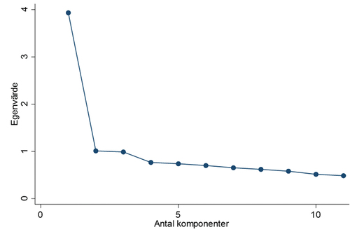
The first factor created is a linear combination of variables that explains most of the total variance of all variables. Subsequent factors are created by linearly combining the variables so that they explain as much of the remaining variance as possible. This process continues until we have created as many factors as we have variables. The number of factors to be retained is determined by a criterion based on the explanation of the variance. Factors with an eigenvalue greater than one are considered significant, and those with an eigenvalue less than one are considered nonsignificant. Significant factors will be used as attributes in the hedonic price equation.

4. Data and descriptive statistics

The empirical analysis will be based on single-family house property sales, with information on the transaction price and various attributes that affect the value. The total number of transactions consists of all sales regarding detached houses in 2021 and spring 2022. Only transactions in urban areas and properties larger than 80 square metres and less than 250 square metres are included in the sample. We have only included older properties, that is, those built at least 30 years ago. Our primary purpose has been to analyse the effect of improvement measures on depreciation rates on older properties, for which we currently have significantly less information on their condition than for newer buildings.

We conducted a stratified sample selection process that resulted in the inclusion of 72 municipalities in our study. This stratification was meticulously carried out to ensure diversity in the sizes of urban areas and housing prices. Our research focused on analysing property transactions within Sweden’s most densely populated urban areas, excluding the city of Stockholm, which is the country’s largest municipality, due to limitations in the number of available surveys. We contacted property owners who had recently purchased real estate to collect data. The survey was distributed to these individuals, with a maximum limit of 15,000 responses.

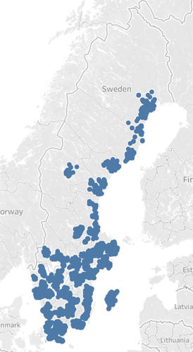
In addition, we included all transactions in real estate older than 30 years within the selected municipalities. Lantmäteriet was pivotal in this data collection process, providing information on transactions and relevant housing attributes that contribute to property values. They also formulated the survey questionnaire, administered it to the respondents, collected the responses, and recorded the data. The outcome of our data collection efforts yielded a total of 9,509 valid survey responses, all of which were meticulously registered. The selected municipalities for our study are visually represented in Map 1, showcasing the geographical distribution of our sample. Our primary focus is to examine real estate transactions within urban areas with high population density in Sweden outside Stockholm. This careful selection and inclusion of property transactions older than 30 years ensure that our analysis captures broad housing market dynamics.

Using a stratified sampling technique improves the reliability of our findings by ensuring that the selected municipalities represent a diverse range of urban areas and variations in housing prices. This approach helps minimise bias and provides a more accurate representation of the target population. Lantmäteriet’s participation in formulating the survey questionnaire, administering it to the respondents, and recording the data contributes to reliability. Their expertise ensures that the questions are well-structured and relevant, potentially reducing measurement error and enhancing the overall quality of responses. Collecting and registering 9,509 valid survey responses indicates a substantial sample size, often associated with greater reliability. A larger sample size generally leads to more robust statistical analyses and enhances the generalisability of your findings. Although the exclusion of Stockholm might limit the scope of your study, it should be noted that this decision was made to ensure the highest quality of data within the constraints of available surveys. This careful consideration of the limitations of the sample size can contribute to the overall reliability of our analysis. The visual representation of the selected municipalities on Map 1 provides a clear overview of the geographical distribution. This document improves transparency and allows readers to assess the spatial coverage of our study, increasing its reliability. The comprehensive approach to data collection, which involves data on transactions, housing attributes, and survey responses, as well as meticulous registration of these responses, adds to the reliability of the study’s dataset.

The included housing attributes are living area, other area and total area, as well as lot size and year of construction. In addition, a quality variable, the quality index, is included, with its various subcomponents. The subcomponents include information on the facade, roof, electricity, windows, bathroom, kitchen, and fireplace. The quality index can range from a maximum of 59 points to a minimum of 6 points, and some of the subcomponents relate to the assessment of maintenance and reconstruction done on the property. To test the robustness of our estimates, we estimate the model with the quality index and an adjusted quality index, where we have excluded components that measure maintenance assessment.

The primary objective of the current study is to evaluate whether additional information on the quality of older single-family homes affected the depreciation factor. The effective age is initially measured using the years of construction and reconstruction. We also have location information consisting of the municipality and geographic coordinates. The descriptive statistics on the included variables are presented in Table 1.

Table 1. Descriptive statistics regarding transaction price and value-affecting attributes (number, mean, standard deviation).

Variable	Number	Average	Standard deviation
Transaction price (SEK)	9509	3,969,116	2,711,460
Living area (square metre)	9509	130.18	33.05
Other area (square metres)	7669	68.56	40.77
Total area (square metres)	9509	140.33	33.44
Lot size (square metres)	9509	1351.71	1536.32
Quality index (index)	9509	32.82	5.76
Adjusted quality index (index)	9509	30.08	3.34
Construction (year)	9509	1956	25
Reconstruction (year)	2248	1994	17
Effective age (year)	9509	1962	33

Note. The table shows descriptive statistics regarding the dependent variable transaction price (krona) and the independent variables living area (square metre), secondary area (square metre) and value area (square metre). Value area refers to living space plus 20% of living space if it can be accessed through the living space. The plot area (area) is also included. In addition, the standard score variable (Skatteverket 2020:4) is also included, an index variable consisting of various subcomponents. The subcomponents consist of information about the property’s building materials and equipment. The exterior components consist of facade cladding, garage and carport, and maintenance and remodelling standards. The energy management group’s subcomponents consist of electricity, windows and heating, and maintenance and remodelling standards. The kitchen refers to equipment and maintenance and remodelling standards. The area of sanitation refers to water, baths, showers and water-flushed toilets, space for washing and clothing care, and maintenance and remodelling standards. Finally, we have other interior attributes such as fireplace and family room. The maximum standard score is 59 points. We also produced an adjusted standard score where the points related to maintenance and rebuilding standards have been excluded. The year of construction referred to when the building was built, and the year of reconstruction refers to when the building has been rebuilt or built into a change to the building’s living space. The year of value will equal the year of construction if the building has not been extended or rebuilt.

The sample includes a total of 9,509 observations. Most of these consist of properties with free-hold land, while some have a leasehold (189). We have information on the transaction price, living area, year of construction and reconstruction, and quality index. Information is missing from many properties for the year of reconstruction and other areas. This may be because some properties lack other areas and have never been reconstructed, or there is no information on any other area and the year of reconstruction.

The average price for a property in the sample is just under SEK 4 million (3,969 KKR), but the variation around the average value is high. The standard deviation is a total of 2.7 million SEK. The variation is due to the properties being in different regions, significantly impacting the price. The average size of the living area is approximately 130 square metres, with a standard deviation of 30 square metres. Thus, the variation in living space is significantly less than that of the transaction price. The average total area is larger (approximately 140 square metres) than the living area since 20% of the other area is counted as the total area. The average quality index is almost 33 points, with a standard deviation of just under 6 points. Here, too, the variation around the mean value is relatively limited. On average, the properties were built in 1956, varying approximately 25 years. However, we can also note that the effective age year is slightly higher (1962). The effective average age would be approximately 59 years.

Additional variables obtained through the survey include the roof, facade, windows, foundation, heating, electricity, drainage, bath, kitchen, and surface layer. For each variable, respondents were asked when they last addressed the issue and to provide a subjective assessment of its condition, either very good or bad. Property owners could respond with information about when the renovation was completed or their subjective assessment of the condition, even if they did not have the information. Since the properties were recently purchased, respondents are not expected to have done the renovations themselves, but rather that information was obtained from previous owners or the broker’s description. The goal was to obtain an assessment of the property’s condition at the time of sale. Descriptive statistics for the included variables are presented in Table 2 (for the assessed year) and Table 3 (for the assessed condition).

Table 2. Supplementary variables and respondent’s information when the measure was introduced (number of respondents).

	Roof	Facade	Window	Foundation	Heating	Electricity	Drainage
2020–2021	328	139	289	162	524	437	306
2011–2019	1386	560	1497	618	1809	852	654
2004–2010	875	316	807	498	1547	407	323
1995–2003	485	204	327	364	693	199	171
1988–1994	184	104	109	133	75	66	88
1981–1987	123	102	93	71	56	67	55
1971–1980	124	190	97	135	53	122	114
Totalt	3505	1615	3219	1981	4757	2150	1711

Table 3. Supplementary variables and respondent’s information when the measure was introduced (number of respondents).

	Bath	Kitchen
2019–2021	829	832
2017–2018	498	487
2014–2016	715	735
2009–2013	824	872
2005–2009	829	790
2000–2004	517	442
1991–1999	376	316
Totalt	4591	4474

Note. The table is divided into two parts (a and b) depending on whether the respondents have had to take a position at different periods regarding the property’s roof, facade, windows, foundation, heating, electricity and drainage, and the property’s bathroom and kitchen. The table shows how many respondents responded when various measures were implemented. The table shows the age ranges; most variables have equivalent age ranges (Table 1). Exceptions are bath and kitchen renovations (Table 3), which are assumed to have a shorter technical and economic lifespan; thus, the age intervals are shorter.

The analysis reveals two notable observations. First, only a small proportion of respondents provided information on the timing of the measures implemented, indicating that they did not have access to this information. For example, only 1615 respondents indicated when the facade was last rebuilt. On the contrary, more respondents could provide information on the dates of kitchen, bath and kitchen renovations, but this only represented less than half of the total survey respondents. Second, the distribution of the responses was skewed, with a higher number of respondents indicating time intervals closer to the purchase date. As the time interval between the renovation and the response to the survey increased, the number of respondents providing information decreased.

In relation to roof, facade, foundation, and heating, less than half of the respondents stated that renovation or replacement work had been carried out in the last five years. However, for windows, electricity, and drainage, more than half of the respondents stated that renovation or replacement work had been carried out in the last five years. Across all types of properties, relatively few property owners indicate that the property in question dates back to the last century, with less than 10% of respondents indicating that the property was rebuilt in whole or in part before 2003.

Table 4 presents the condition of the assessment of the property by the property owners at the time of purchase. Respondents unaware of when maintenance and reconstruction had been performed were asked to assess the condition on a six-point scale ranging from much better than normal to much worse. The results are presented in Table 4.

Table 4. Supplementary variables and the respondent’s subjective assessment (number of respondents).

	Roof	Facade	Window	Foundation	Heating	Electricity	Drainage	Bath	Kitchen	Surface
Much better than normal	64	70	100	65	82	61	52	65	92	240
Better than Normal	161	297	276	222	240	155	125	169	236	745
Normal	1845	4245	2155	4235	2136	3499	4524	1346	1644	4428
Somewhat worse than normal	1063	1409	1201	1267	598	1323	1355	604	684	2091
Worse than normal	1705	1137	1487	942	704	1162	934	1204	1200	1291
Much worse than normal	1004	552	936	620	838	934	621	1398	1034	541
Total	5842	7710	6155	7351	4598	7134	7601	4786	4890	9336

Note. The questions regarding the respective property were first referred to when the action was carried out within a time interval. If the respondent has not had the information, they have been asked to give a subjective assessment regarding the roof, facade, windows, foundation, heating, electricity, drainage, bath, kitchen, and surface layer. The respondent has assessed the property on six levels: (1) The property had several defects and is assessed as very poor. Replacement in the property probably needs to be done soon (0–4 years), (2) the property had some shortcomings, and the condition is considered worse than normal. A replacement in the property probably needs to be done within 5–10 years, (3) the property was acceptable, and the condition is assessed to be somewhat worse than normal. A change of property is judged to be farther away than ten years away in time, (4) the property was good, and the condition is judged to be better than normal, (5) the property was very good, and the condition is judged to be better than normal, and (6) the property was excellent, and the condition is rated as much better than normal. The table shows the number of people who have answered the respective question and judgement and the total.

Based on the results of the survey, it can be concluded that only a small percentage of property owners know when maintenance and investments have been made on their property. Most respondents have instead provided subjective assessments of the property’s condition, which may vary depending on the individual’s perception of normality. However, despite subjectivity, information on the condition is still considered valuable. It is worth noting that in a market with many transactions, the consensus on the condition of individual properties tends to converge towards what the market considers normal.

The survey results also suggest that it is relatively easier for property owners to indicate the year when work has been done on the kitchen and bathroom, while it is more challenging to indicate when work has been done on the facade, foundation, electricity, and drainage. In particular, less than 10% of respondents indicated that their property was replaced in whole or part before 2003, suggesting that most properties are relatively new.

In terms of these characteristics, it can be observed that approximately 80% of the respondents have provided an assessment rather than specifying a period. Furthermore, it can be observed that for these characteristics, most respondents have indicated that the condition is average in terms of the number of responses and, in comparison, the total number of assessments made. Few respondents have indicated that the condition is much better or better than normal, with less than 10% indicating this, while 20–30% have indicated that the condition is worse or worse than average.

Regarding the features that property owners believe will require maintenance in the next 10 years, it can be seen that the facade, foundation, heating, electricity, drainage, and surface layer are characteristics that most people believe require relatively little attention. On the other hand, more than half of the respondents believe that maintenance will be needed for the windows, roof, bath, and kitchen, which may be because these characteristics are easier to assess. In contrast, evaluating the condition of the foundation, electricity, heating, and drainage is much more challenging.

To enable comparison of the answers (age range or subjective assessment), we have ‘translated’ the subjective assessment to a year where the normal standard indicates a year of 30 years. If the property is much worse than normal, we set the value at 50 years; if it is much better than normal, we set the value at ten years. With regard to the age range, we have used the middle value, i.e. the age group 1971–1980 has a number of years equivalent to 45 years. Through this procedure, we have analysed the various subcomponents regardless of whether the respondent has answered with an age range or made a subjective assessment. The new effective age² was then calculated as an average value of all subcomponents of equal weight.

The variables included in the analysis have a high mutual correlation, particularly those that measure age and quality, such as the year of construction, the year of reconstruction, the quality index, and additional variables related to the roof, facade, windows, foundation, heating, electricity, drainage, bath, kitchen, and surface layer.

Table 5 presents the correlations between the new additional variables. The correlation matrix reveals a strong positive correlation between the additional variables, indicating that if one variable is in good condition, the others are also likely to be in good condition, such as the roof (T) and the facade (FA). The strongest positive correlation is observed between the effective age of wastewater (A) and electricity (E), suggesting that if the effective age of drainage is high, the effective age of electricity is also likely to be high. This connection between sewer/electricity is also stronger compared to the kitchen (K) and bath (B), which are highly correlated with the surface layer (Y), which is reasonable. On the contrary, we observe the lowest correlation between the effective age of the roof, the kitchen, and the surface layer. All variables have a positive and statistically significant correlation, indicating that they partly measure the same underlying construct. Based on the correlation matrix, we expect it to be possible to reduce the number of factors we have analysed in the factor analysis.

Table 5. Correlation matrix.

Note. The table shows the correlation between the independent variables. The correlation coefficient is from −1 to + 1 (from a perfect negative to positive relationship). The blue cell indicates a lower correlation between the variables, and the red cell shows a higher correlation. The variables refer to the roof (T), facade (FA), window (FO), foundation (G), heating (V), energy (E), drainage (A), bathroom (B), kitchen (K) and general surface layer (Y). All correlation coefficients are statistically significant on a 5% level.

The factor analysis was conducted using a principal component analysis with ten supplementary variables that indicate when measures have been carried out or the property’s condition. The effective age, based on the difference between the year of sale and the year of construction or reconstruction, was also included in the factor analysis. According to the literature, a sample size of at least 10:1 is recommended for factor analysis (Hair et al., 2006), although a ratio of 20:1 is also observed. Our dataset is large enough to perform factor analysis. Table 6 presents the results of the analysis of the main components.

Table 6. Principal component analysis.

Component	Eigenvalue	Share	Cumulative
F1	3.984	0.3622	0.3622
F2	1.04942	0.0954	0.4576
F3	0.951292	0.0865	0.5441
F4	0.755571	0.0687	0.6128
F5	0.738376	0.0671	0.6799
F6	0.689016	0.0626	0.7425
F7	0.651691	0.0592	0.8018
F8	0.614181	0.0558	0.8576
F9	0.570467	0.0519	0.9095
F10	0.513602	0.0467	0.9561
F11	0.482382	0.0439	1.000

Note. The table reproduces the eigenvalues for each factor (F1-F11) estimated using the principal component analysis. Proportion refers to how much each factor explains the total variation (variance) in the data material concerning the investigated variables. Cumulative refers to the cumulative summation of the shares, and all factors explain 100% of the total variation.

The first principal component has the highest eigenvalue and explains the highest proportion of total variation among the 11 variables. It accounts for approximately 36% of the total variation; the second component explains almost 10%, and the third component explains just under 9%. The first three components combined explain approximately 54% of the variation. The relationship between the number of components and the eigenvalue is illustrated in Figure 1 (in the Appendix). As the number of components increases, the intrinsic value decreases. Earlier, we mentioned that the criterion for determining the number of components to analyse further is one. In this case, the first two components are above one, while the third is borderline. We also calculated the Kaiser-Meyer-Olkin measure to assess the suitability of the sample (sampling adequacy). Our estimate is 0.9042, higher than 0.5, indicating that our data are suitable for the chosen method.

Table 7 presents the eigenvector, which shows the degree to which the different variables are associated with the various components. The weights in the eigenvector represent the coefficients in the linear combination of the constituent variables included in each component.

Table 7. The components (eigenvector).

	F1	F2	F3
Roof	0.2527	−0.3828	0.4678
Facade	0.3171	−0.1330	0.3492
Window	0.3026	−0.1104	0.2981
Foundation	0.2994	−0.0471	0.2628
Heating	0.2814	−0.1196	−0.0834
Electricity	0.3597	0.0140	−0.2135
Drainage	0.3358	−0.0176	−0.2859
Bath	0.3395	0.1416	−0.2345
Kitchen	0.3345	0.2220	−0.2866
Surface	0.3236	0.2148	−0.1308
Age	0.0350	0.8313	0.4615

Note. The table shows how the factors/components have been defined. Only the first three components are reproduced in the table (those with an eigenvalue approximately equal to 1). The values in the table refer to the weight of the respective variable in the factors/components created. The weights can be negative or positive. The correlation between F1-F3 is, by definition, equal to zero (0).

The analysis suggests that there are at least three distinct components. Component 1 includes the additional variables, with relatively equal weighting between them, although the roofs have a slightly lower weight. Component 2 includes the effective age,³ as well as kitchens, baths, and finishes. Roofs have a negative impact on component 2. Component 3 mainly includes roofs, facades, windows, and foundations, representing external maintenance/condition. The internal condition has a negative impact on this component. In summary, component 1 (name: all conditions) includes additional information, component 2 (name: interior conditions) includes existing information on effective age, and component 3 (name: external conditions) includes external conditions.

5. Econometric analysis

The empirical analysis will be conducted in several stages. In Step 1, a base model will be estimated using only available information, and in Step 2, a variable will be included in the extended model based on the supplementary variables (variable name: new effective age). In the third model, components of the factor analysis will be included in the model. As an alternative, two types of stepwise models will be estimated in Step 3, where the included variables are selected based on their statistical significance. Finally, two models will be estimated to test the heterogeneity of parameter estimates for the new effective age. This will be done through a cohort model, testing whether the estimates vary across different cohorts, and a quartile model, testing whether the estimates vary across the price distributions.

5.1. The hedonic regression model

In Tables 8 and 9, we present the results of the basic model, the extended model and the factor model, while in Table 10, we present the results from stepwise regressions, the results from the heterogeneity models. We will focus on the individual parameter estimates regarding the variables relating to effective age, the model’s degree of explanation (in-sample) and the model’s predictive ability (out-of-sample).

Table 8. Hedonic price models.

	(1)	(2)	(3)
Effective age	−0.00179***	−0.00423***
	(−3.49)	(−8.32)
Effective age squared	0.00000289	0.0000241***
	(0.68)	(5.64)
Lot size	0.00000952	0.00000935	0.0000104*
	(1.91)	(1.87)	(2.13)
Living area	0.00376***	0.00345***	0.00363***
	(33.64)	(29.93)	(32.17)
Quality index	0.0121***
	(18.94)
Adjusted quality index		0.0221***	0.0211***
		(18.38)	(18.16)
New effective age			0.00773***
			(4.24)
New effective age squared			−0.000303***
			(−8.44)
R^2	0.815	0.815	0.820
Adjusted R^2	0.798	0.798	0.804
RMSE (insample)	0.276	0.276	0.272
RMSE (out-of-sample)	0.270	0.267	0.264
Observations	7187	7187	7187

Note. The table reproduces the results of five regressions where we have added information on the condition. Model (1) refers to the base model where the new variables are not included. In addition to the independent variables, plot area, value area, standard score, fixed area and time effects, and effective age and squared are also included. The age is defined based on the year of construction or reconstruction. Model (2) refers to the same model but where information about the condition in the standard score has been excluded. Model (3) includes information regarding the added variables of effective age and squared. The variable new effective age refers to an unweighted average of the variables of renovations. The table shows the respective variable’s coefficient estimate and t-value in parentheses. The models also include fixed-area and time effects. Each coefficient estimate also provides an indication depending on its significance with * p < 0.05, ** p < 0.01, *** p < 0.001. The model’s explanatory power is indicated by R², adjusted R² and its predictive power by RMSE (in-sample) and RMSE (out-of-sample). In addition, the number of observations is reproduced.

Table 9. Hedonic factor models.

	(1)	(2)	(3)
Lot size	0.00000981*	0.0000139**	0.0000145**
	(2.02)	(2.85)	(2.98)
Total living area	0.00364***	0.00357***	0.00357***
	(32.20)	(31.65)	(31.70)
Adjusted quality index	0.0217***	0.0201***	0.0198***
	(18.76)	(17.14)	(16.91)
Component 1 (all conditions)	−0.0293***	−0.0296***	−0.0297***
	(−17.13)	(−17.39)	(−17.47)
Component 2 (interior conditions)		−0.0289***	−0.0294***
		(−8.11)	(−8.28)
Component 3 (external conditions)			−0.0171***
			(−5.01)
R^2	0.819	0.821	0.822
Adjusted R^2	0.802	0.804	0.805
RMSE (insample)	0.273	0.272	0.271
RMSE (out-of-sample)	0.264	0.264	0.263
Observations	7187	7187	7187

Note. The table reproduces the results of three regressions where we have added information on the condition, in addition to the independent variables, plot area, value area, standard score, fixed area, and time effects. The effective age and effective age squared variables are not included in the models as they are included in the factor analysis. Model (1) refers to a model in which factor 1 (F1) is included, model 2 includes F1 and F3, and finally, all factors (F1-F3) are included in model 3. The table shows the respective variable’s coefficient estimate and t-value in parentheses. The models also include fixed-area and time effects. Each coefficient estimate also provides an indication depending on its significance with * p < 0.05, ** p < 0.01, *** p < 0.001. The model’s explanatory power is indicated by R², adjusted R² and its predictive power by RMSE (in-sample) and RMSE (out-of-sample). In addition, the number of observations is reproduced.

Table 10. Cohort analysis.

	(1)	(2)	(3)	(4)
	−1939	1940–1964	1965–1974	1975-
Lot size	0.0000209*	0.0000289*	0.0000106	0.0000260**
	(2.32)	(2.15)	(0.62)	(2.58)
Total living area	0.00385***	0.00364***	0.00317***	0.00290***
	(15.19)	(15.62)	(12.79)	(12.16)
Adjusted quality index	0.0242***	0.0214***	0.0190***	0.0131***
	(7.89)	(9.42)	(8.28)	(4.95)
New effective age	0.0192***	0.00563	0.00310	0.00505
	(3.95)	(1.59)	(0.90)	(1.41)
Average new effective age squared	−0.000532***	−0.000266***	−0.000207**	−0.000234***
	(−5.65)	(−3.78)	(−3.05)	(−3.33)
R^2	0.852	0.871	0.867	0.868
Adjusted R^2	0.798	0.833	0.824	0.825
RMSE (insample)	0.315	0.266	0.232	0.221
Observations	1694	1993	1736	1764

Note. The table shows the results from our cohort analyses. We divided the material by year of construction and created four cohorts. The first refers to buildings built before 1940; the second refers to buildings built between 1940 and 1965; the third refers to buildings built between 1965 and 1975; and the last cohort refers to buildings built after 1975 (but before 1992). The model includes lot size, total living area, adjusted quality index and new effective age with equal weights. The t-values show the statistical significance in parentheses. Absolute values above 1.96 mean the parameter estimate is statistically significant at a 5% significance level. Significance is also given by: * p < 0.05, ** p < 0.01, *** p < 0.001. The models include fixed area effects and time effects. The model also includes effective age based on the year of construction or remodelling. R², adjusted R² and RMSE indicate the explanatory power of the model. In addition, the number of observations is reproduced.

The degree of explanation (R²) is 0.815, indicating that independent variables can explain 81.5% of the price variation. Adjusted R² is slightly lower at 79.8%. This level of explanation is relatively good and can be found in many hedonic studies. However, the predictive ability of the model is relatively poor, with an RMSE of 0.276. Since the dependent variable is the transaction price in logarithmic form, this value can be interpreted as the average prediction error corresponding to 27.6%.

The estimate of the effective age in column 1 is statistically significant and negative, indicating that older properties have lower prices. The effective age is calculated as the year of sale minus the highest value of the year of construction or reconstruction. However, the squared effective age is not statistically significant. The parameter estimate of the effective age is relatively low, only 0.18% per year. The results in column 2 use the same effective age, but use the adjusted quality index as an independent variable.

The probable explanation for the relatively low parameter estimate concerning the effective age in the base model is twofold. First, we are analysing properties with a construction year older than 30 years, which means that a substantial part of the year-related decrease in value has already occurred in the first 30 years. Second, we do not account for the condition of the property in the model; although the quality index variable is included, it measures more the occurrence of various attributes than the property’s condition.

The second model (column 2), which includes an adjusted quality index instead of a standard score, shows similar results in terms of predictive ability as the first model. However, the estimated depreciation factor in the second model differs from that of the first model. The reason for this is that the second model considers the property’s condition through the adjusted standard score, whereas the first model does not. If we do not control for the condition, the estimated depreciation factor will be significantly higher. This finding is consistent with previous studies that demonstrate the impact of a property’s condition on the estimated depreciation factor.

The extended model (column 3) includes the average effective age (also squared) based on the ten additional questions and the effective age. The model shows a slightly higher degree of explanation (from 79.8 to 80.5%). The average prediction error decreases slightly, indicating that information from the supplementary questions moderately impacts predictive ability. However, it should be noted that the individual coefficient estimates are statistically significant.

Surprisingly, the estimate of the effective age based on the supplementary questions is positive, indicating an increase in value of 1% per year. However, the squared term is statistically significant and negative, suggesting a decrease in value over time, but initially there is an increase in value. The correlation between the variables may partially explain the unexpected results. The assumption of equal weights in the average effective age regarding the supplementary questions may not be appropriate due to multicollinearity between the variables that measure effective age, each based on the year of construction or the supplementary questions. Therefore, it may be necessary to perform a factor analysis to explore further the relationships between the variables and their impact on the model’s performance.

The comparison between columns (1) and (3) in Table 8 and the visualisation of the age effect in Figure 1 reveal a significant difference in the age-related decrease in value for properties over 30 years of age. The base model, which does not consider reinvestments and conditions, shows a relatively constant depreciation rate for properties older than 30 years. However, using the effective age instead of the age in the model yields a different depreciation pattern. At around 30 years, both models’ depreciation rates are the same. However, after 30 years, the depreciation rate increases significantly when the age is measured with the effective age. For a property built more than 30 years ago with an effective age of 1 year, its value will increase over a few years and decrease around an effective age of 15. At an effective age of 30, the depreciation factor is less than 0.1% per year, which increases to 0.2% at an effective age of 40 years and approximately 0.6% per year at 60 years. It should be noted that there is considerable uncertainty in the estimates for effective ages over 50 years.

Figure 1. Included transactions distributed across Sweden.

How should we interpret these results? On the basis of the effective age, excluding renovations, the annual depreciation is low, as expected. If, on the other hand, renovations have taken place and made the property younger, measured as effective age, we will instead have an appreciation. It could be a result of a vintage effect; that is, older properties could have a positive vintage effect, but only if the property is well maintained. The interpretation could also be that it is profitable for the individual owner of an older property to physically renovate and maintain their older property.

Previous studies have estimated the depreciation rate for properties of different ages and conditions. For instance (Shilling et al., 1991), estimated the depreciation factor at around 1% for a 10-year-old property, while (Malpezzi et al., 1987) estimated the factor at only 0.4%. Wilhelmsson (2008) estimates the depreciation factor for well-maintained and less-maintained properties at 20 and 40 years, respectively. The depreciation factor for well-maintained properties is around 0.3% at 20 years, while at 40 years, there is an appreciation effect of 0.1% per year. The corresponding values for less-maintained properties are 0.7% and 0.2% per year. Therefore, considering that we are analysing older properties, the estimates in the base model are consistent with previous studies.

5.2. The factor regression model

The results of the factor model in Table 9 reveal that the model has explanatory power as the extended and base models, with only a slight improvement. However, this difference is not statistically significant. All three components or factors exhibit statistically significant parameter estimates with the anticipated direction of influence. This means that if the component increases in value, it has a negative impact on the property’s value. F1 has the highest statistical significance, followed by F2 and F3. However, F2 has the most substantial impact on value, with a predicted decrease of 3% for a unit increase in the component. Interpreting these results in economic terms can be challenging, which is a common problem with incorporating components from factor analysis into the hedonic price equation. We assess that factor analysis shows that all subcomponents have the same weight and that using an average effective age with equal weights can be a reasonable way to go.

Based on the results of the stepwise regressions, it appears that each variable contributes to explaining the price variation, with 7–8 out of the 10 variables showing statistically significant parameter estimates. Furthermore, the expected sign of the effect is observed for all variables (except drainage), indicating that a worse condition has a negative impact on the price. Furthermore, variables such as time since investment and assessed condition have an expected negative effect on the price, indicating that long time since investment or a worse assessed condition will result in a lower price. However, the parameter estimates are relatively low, suggesting that the impact of each variable is relatively marginal.

5.3. Parameter heterogeneity models

We have estimated the effect of depreciation within different cohorts with respect to the year of construction. The result is presented in Table 10.

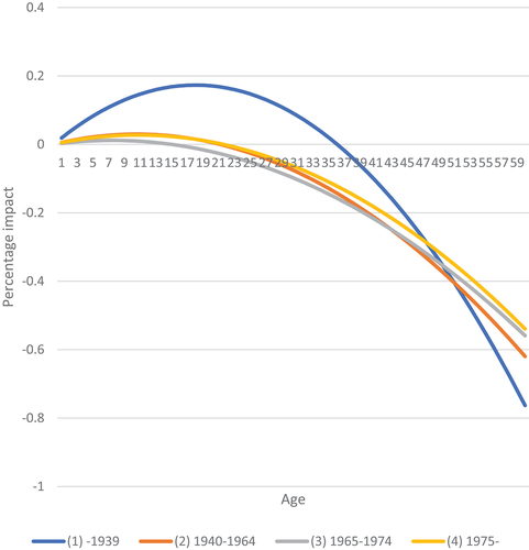
The cohorts used in this study are as follows: before 1939, 1940–1964, 1965–1974, and 1975 and later. The division was carried out to ensure equal sample sizes in each cohort. We can also see that age classes are associated with different architectural styles. Before 1940, single-family houses were dominated by the functionalism that started around 1930. Older single-family houses can be divided into classicism, romantic national style, and art nouveau style. During the 1949-50s, the style was, above all, functionalism to be followed by more prefabricated single-family houses and terraced and terraced houses to a greater extent during the 1960s. During the 1970s, single-family houses were characterised by 1–1/2-story houses without basements, usually built of wood.

The variables of interest are the new effective age. The effect differs between cohorts. For buildings built before 1940, the value initially increases if the effective age increases by one year and then decreases. However, we did not observe a corresponding positive price effect in the other cohorts.

Previously, we interpreted the result as an appreciation effect on older properties that have been renovated and made the effective age lower, that is, there is a positive vintage effect. The results of the cohort analysis show that this does not apply to all older properties, except for those built before 1940. For younger properties, the effect is marginal. It can be interpreted as only properties that were built more than 80 years ago where it pays less to renovate and maintain the property.

Therefore, an interpretation is that there is a positive vintage effect for older buildings, but not for those built after 1940. However, the negative coefficient estimates regarding the effective age squared suggest that the decrease in value due to poorer conditions is more significant for the oldest properties. This effect is reflected in Figure 2 and in Figure 3 is the effect shown in different cohorts.

Figure 2. Age depreciation without (base model) and with consideration of condition (effective age).

Note. Figure 1 graphically reproduces the effect of age on housing value. The graph is based on the coefficient estimates in Table 7 regarding the variables effective age and effective age squared (model 1) and the new effective age and new effective age squared (model 3).

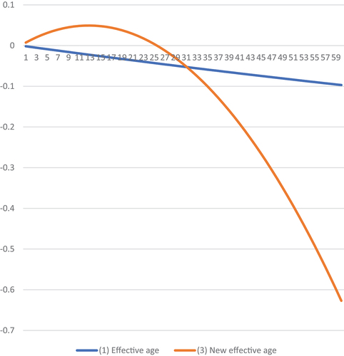
Figure 3. Depreciation rate within different cohorts.

Note. We divided the material into four different age groups (cohorts). Buildings built before 1940, between 1940-1965, 1965-1975 and 1975. The figure is based on the estimates in Table 9 (columns 1-4). On the vertical axis, we have the rate of depreciation per year measured in percentage, and on the horizontal axis, we have the effective age.

6. Conclusions and implications for policy

We know that properties lose value with age, but renovations and maintenance can reduce age-related depreciation. A large proportion of our housing stock consists of properties older than 30 years, but at the same time, we know less about their condition than newer properties. The variation in the condition of the older properties is also greater. Therefore, the research question is whether it is possible to collect more information from property owners to better understand the depreciation rates for older properties.

From the literature review, we can state that many articles from different countries have analysed the issue of age-related depreciation and the importance of maintenance and renovations. Several methods have been used in these studies to estimate the degree of depreciation, but the hedonic methodology is the most used. These studies show that the depreciation rate varies depending on many factors, including how well the property owner has taken care of the property.

The empirical literature shows an average decrease in value of 1 to 2% per year, depending on the housing market. There is also support in the empirical literature that a well-maintained property has a depreciation factor of less than 1%, while a property in worse condition can have a depreciation factor of more than 3%. We can also note in the literature that the age-related decrease in value is most evident in the first years after a building; the decrease in value is not linear over time. There are indications that the depreciation differs between properties depending on the construction period (the so-called cohort effects).

In our empirical analysis, a hedonic regression model was estimated to examine the impact of effective age on property prices. The results indicate that the effective age has a statistically significant negative impact on property prices, estimated at only 0.18% per year. However, the squared effective age is not statistically significant, indicating that there is no vintage effect. The low-parameter estimate of effective age can be explained by the fact that the properties analysed are already over 30 years old, and a substantial part of the year-related decrease in value has already occurred. Furthermore, the model does not account for the condition of the property. The degree of explanation of the model is relatively good, but the predictive ability is relatively poor.

The purpose of the study is to evaluate whether additional information about the quality of older single-family homes affected the depreciation factor, as we have less knowledge of the renovations have been carried out for older properties. We address the research question by supplementing existing register data with a survey of the property owners and what has been done in the property when they bought it. Of course, this is a subjective assessment of the property’s condition, which can differ greatly depending on the person. It limits our interpretation of the valuation model in relation to whether these further, more subjective judgements about the property’s condition add anything. Our conclusion is, in part, that it does not.

In the extended model, we have included a new effective age based on ten additional questions, showing a slightly higher degree of explanation and a moderate impact on the model’s predictive ability. However, the estimates of the individual coefficients of the model were statistically significant and the estimate for the new effective age was positive, indicating an increase in value of 1% per year. The factor model, which included components of factor analysis, showed similar results to the extended model. The model that considered the condition through the adjusted standard score showed a lower estimated depreciation factor, consistent with previous studies.

The results of this empirical analysis could have several policy implications. First, the finding that older properties have lower depreciation rates could be helpful for policymakers in the housing sector, particularly those interested in urban renewal and regeneration. It suggests that measures to stimulate the renovation and renovation of older properties could effectively increase their value and potentially revitalise urban areas. Second, the results suggest that the condition of a property is an essential factor in determining its value, which could be relevant for policymakers concerned with building codes and regulations. Policies that aim to improve the maintenance and upkeep of properties could help increase their value and improve overall housing quality. Third, we find that the model’s explanatory power is relatively high, but its predictive ability is relatively poor, suggesting that some unmeasured attributes influencing the housing market are not considered in the model. Policymakers may need to consider additional variables or conduct further research to better understand these factors and their impact on the housing market.

Acknowledgements

The project was carried out on behalf of the Land Surveying Agency. They have provided financial funding and data for the project.

Disclosure statement

No potential conflict of interest was reported by the author(s).

Additional information

Funding

The work was supported by the Lanmäteriet Lantmäteriet .

Notes on contributors

Mats Wilhelmsson

Mats Wilhelmsson, Associate Professor in Real Estate Economics at Royal Institute of Technology (KTH), Stockholm, Sweden. I have a bachelor degree in Economics from StockholmUniversity and a PhD-degree in Real Estate Economics from KTH. I am Head of the Division of Building and Real Estate Economics, at the Department of Real Estate and Construction Management, KTH. My research is focused on housing and urban economics, and innovation studies. Present research areas are innovation network and its impact on innovations, explaining the spatial distribution of patents and networks, and estimating the housing supply. Earlier work on housing markets has considered the consumption of various components of housing services and the relationship of disaggregated consumption to market prices for housing units; analysis of housing submarkets; spatial models concerning house price determination; and vacancy rates under a rent control regime.

Notes

1. The effective age of a property is based on when it was built and when major renovations or extensions have been made. A property that has not changed since it was built has an effective age of year of sale minus year of construction. If, on the other hand, the property has been renovated, this will reduce the effective age. A fully renovated property will have a low effective age even if the property was originally built in the 1940s and is 80 years old.

2. The new effective age refers to the age of the property at the time of sale but corrected for the information on renovations that has been collected via the survey.

3. Effective age is based on register information concerning year och construction and year of renovation.

Appendix

Figure 1. Screeplot of eigenvalue by number of components.

Note. The figure (screeplot) shows the relationship between the eigenvalue and the number of factors/components. The more factors, the lower the eigenvalue is. The values are the same as the eigenvalues in Table 5, and the inclusion criterion equals eigenvalue one (1).

References

- Arnott, R., Davidson, R., & Pines, D. (1983). Housing quality, maintenance and rehabilitation. The Review of Economic Studies, 50(3), 467–494. https://doi.org/10.2307/2297676
- Baum, A. (1993). Quality, depreciation, and property performance. Journal of Real Estate Research, 8(4), 541–565. https://doi.org/10.1080/10835547.1993.12090722
- Bhattacharjee, A., Castro, E., & Marques, J. (2012). Spatial interactions in hedonic pricing models: The Urban Housing Market of Aveiro, Portugal. Spatial Economic Analysis, 7(1), 133–167. https://doi.org/10.1080/17421772.2011.647058
- Bokhari, S., & Geltner, D. (2018). Characteristics of depreciation in commercial and multifamily property: An investment perspective. Real Estate Economics, 46(4), 745–782. https://doi.org/10.1111/1540-6229.12156
- Bowie, N. (1984). The DEPRECIATION of BUILDINGS. Journal of Valuation, 2(1), 5–13. https://doi.org/10.1108/eb007944
- Chinloy, P. (1979). The estimation of net depreciation rates on housing. Journal of Urban Economics, 6(4), 432–443. https://doi.org/10.1016/0094-1190(79)90023-8
- Chinloy, P. (1980). The effect of maintenance expenditures on the measurement of depreciation in housing. Journal of Urban Economics, 8(1), 86–107. https://doi.org/10.1016/0094-1190(80)90057-1
- Coulson, N. E., & McMillen, D. P. (2008). Estimating time, age and vintage effects in housing prices. Journal of Housing Economics, 17(2), 138–151. https://doi.org/10.1016/j.jhe.2008.03.002
- Crosby, N., Devaney, S., & Law, V. (2012). Rental depreciation and capital expenditure in the UK commercial real estate market, 1993–2009. Journal of Property Research, 29(3), 227–246. https://doi.org/10.1080/09599916.2012.679009
- Des Rosiers, F., Thériault, M., & Villeneuve, P. (2000). Sorting out access and neighbourhood factors in hedonic price modelling. Journal of Property Investment & Finance, 18(3), 291–315. https://doi.org/10.1108/14635780010338245
- Diewert, E., & Shimizu, C. (2015). A conceptual framework for commercial property price indexes. Journal of Statistical Science and Application, 3(5). https://doi.org/10.17265/2328-224X/2015.910.001
- Diewert, W. E., & Fox, K. J. (2016). Sunk costs and the measurement of commercial property depreciation. Canadian Journal of Economics/Revue canadienne d’économique, 49(4), 1340–1366. https://doi.org/10.1111/caje.12236
- Diewert, W. E., Fox, K. J., & Shimizu, C. (2016). Commercial property price indexes and the system of national accounts. Journal of Economic Surveys, 30(5), 913–943. https://doi.org/10.1111/joes.12117
- Dildine, L. L., & Massey, F. A. (1974). Dynamic Model of Private incentives to housing maintenance. Southern Economic Journal, 40(4), 631–639. https://doi.org/10.2307/1056381
- Dixon, T., Law, V., & Cooper, J. 1999. The dynamics and measurement of commercial property depreciation in the CEM Reading, date last Retrieved November 9, 2023, at http://www.cem.ac.uk/research/reports-publications/the-dynamics-and-measurement-of-commercial-property-depreciation-in-the-uk.aspx
- Downie, M.-L., & Robson, G. 2008. Automated Valuation Models: An International Perspective, https://nrl.northumbria.ac.uk/id/eprint/1683/(date last Retrieved November 7, 2023)
- Ellison, L., & Sayce, S. (2007). Assessing sustainability in the existing commercial property stock: Establishing sustainability criteria relevant for the commercial property investment sector. Property Management, 25(3), 287–304. https://doi.org/10.1108/02637470710753648
- Goodman, A. C., & Kawai, M. (1984). Functional form and Rental Housing Market Analysis. Urban Studies, 21(4), 367–376. https://doi.org/10.1080/00420988420080761
- Gröbel, S. (2018). Regional heterogeneity in age-related housing depreciation rates. Review of Regional Research, 38(2), 219–254. https://doi.org/10.1007/s10037-018-0125-3
- Hair, J. F., Black, W. C., Babin, B. J., Anderson, R. E., & Tatham, R. L. (2006). Multivariate data analysis. Pearson Prentice Hall.
- Harding, J. P., Rosenthal, S. S., & Sirmans, C. F. (2007). Depreciation of housing capital, maintenance, and house price inflation: Estimates from a repeat sales model. Journal of Urban Economics, 61(2), 193–217. https://doi.org/10.1016/j.jue.2006.07.007
- Knight, J. R., & Sirmans, C. F. (1996). Depreciation, maintenance, and housing prices. Journal of Housing Economics, 5(4), 369–389. https://doi.org/10.1006/jhec.1996.0019
- Leigh, W. A. (1980). Economic depreciation of the residential housing stock of the United States, 1950-1970. The Review of Economics and Statistics, 62(2), 200–206. https://doi.org/10.2307/1924745
- Lopez, L. A., & Yoshida, J. (2022). Estimating housing rent depreciation for inflation adjustments. Regional Science and Urban Economics, 95, 103733. https://doi.org/10.1016/j.regsciurbeco.2021.103733
- Lowry, I. S. (1960). Filtering and housing standards: A conceptual analysis. Land Economics, 36(4), 362–370. https://doi.org/10.2307/3144430
- Malpezzi, S., Ozanne, L., & Thibodeau, T. G. (1987). Microeconomic estimates of housing depreciation. Land Economics, 63(4), 372–385. https://doi.org/10.2307/3146294
- Mandell, S., & Wilhelmsson, M. (2011). Willingness to pay for sustainable housing. Journal of Housing Research, 20(1), 35–51. https://doi.org/10.1080/10835547.2011.12092034
- Manganelli, B. (2013). Maintenance, building depreciation and land rent. Applied Mechanics & Materials Trans.Tech Publ, 2207–2214. https://doi.org/10.4028/www.scientific.net/AMM.357-360.2207
- Margolis, S. E. (1982). Depreciation of housing: An empirical consideration of the filtering hypothesis. The Review of Economics and Statistics, 64(1), 90–96. https://doi.org/10.2307/1937947
- Mayer, M., Bourassa, S. C., Hoesli, M., & Scognamiglio, D. (2019). Estimation and updating methods for hedonic valuation. Journal of European Real Estate Research, 12(1), 134–150. https://doi.org/10.1108/JERER-08-2018-0035
- Pagourtzi, E., Assimakopoulos, V., Hatzichristos, T., & French, N. (2003). Real estate appraisal: a review of valuation methods. Journal of Property Investment & Finance, 21(4), 383–401. https://doi.org/10.1108/14635780310483656
- Rolheiser, L., van Dijk, D., & van de Minne, A. (2020). Housing vintage and price dynamics. Regional Science and Urban Economics, 84, 103569. https://doi.org/10.1016/j.regsciurbeco.2020.103569
- Rosen, S. (1974). Hedonic prices and implicit markets: Product differentiation in pure competition. Journal of Political Economy, 82(1), 34–55. https://doi.org/10.1086/260169
- Shilling, J. D., Sirmans, C. F., & Dombrow, J. F. (1991). Measuring depreciation in single-family rental and owner-occupied housing. Journal of Housing Economics, 1(4), 368–383. https://doi.org/10.1016/S1051-1377(05)80018-X
- Shultz, S. (2018). Housing depreciation revisited: Hedonic price modeling versus Assessor estimates. Journal of Housing Research, 27(1), 45–58. https://doi.org/10.1080/10835547.2018.12092140
- Skatteverket. (2020). Författningssamling , 4.
- Smith, B. C. (2004). Economic depreciation of residential real estate: Microlevel space and time analysis. Real Estate Economics, 32(1), 161–180. https://doi.org/10.1111/j.1080-8620.2004.00087.x
- Suzuki, M., & Asami, Y. (2022). The rapid economic depreciation at an early stage of building life among Japanese detached houses. Habitat International, 126, 102600. https://doi.org/10.1016/j.habitatint.2022.102600
- Syed, I. A., & De Haan, J. (2017). Age, time, vintage, and price indexes: Measuring the depreciation pattern of houses. Economic Inquiry, 55(1), 580–600. https://doi.org/10.1111/ecin.12383
- Tretton, D. (2007). Where is the world of property valuation for taxation purposes going? Journal of Property Investment & Finance (Vol. 25, pp. 482–514).
- Wilhelmsson, M. (2008). House price depreciation rates and level of maintenance. Journal of Housing Economics, 17(1), 88–101. https://doi.org/10.1016/j.jhe.2007.09.001
- Yoshida, J. (2016). Structure depreciation and the Production of Real Estate Services. SSRN Electronic Journal. https://doi.org/10.2139/ssrn.2734555
- Yoshida, J. (2020). The economic depreciation of real estate: Cross-sectional variations and their return implications. Pacific-Basin Finance Journal, 61, 101290. https://doi.org/10.1016/j.pacfin.2020.101290