Fireside corrosion and deposition on heat exchangers in biomass combustion systems

ABSTRACT

To address climate change, power plants need to switch to greener fuels. One possible fuel is biomass; a carbon neutral/low carbon fuel. However biomasses’ chemistries are both different from coal’s and vary depending on their sources, containing unique levels of the trace elements (e.g., Cl and S) capable of altering the degradation of heat-exchangers. As such, an understanding of the effects of these variations on fireside corrosion is needed. Laboratory testing exposed alloys T91 and TP347HFG in a simulated agricultural product combustion environment at 600°C (up to 1000h; 100h cycles). Three different deposits mixtures were investigated (comprised of KCl, K2SO4, Na2SO4, CaSO4 indifferent percentages) mimicking accelerated corrosion from different biomasses. Corrosion behaviour was found to be dependant on both alloy and deposit chemistries, with the two materials showing different responses. The deposit with lowest KCl showed lowest corrosion damage, while the highest KCl deposit showed more aggressive behaviour.

KEYWORDS:

• Biomass
• Fireside Corrosion
• heat exchangers
• T91
• TP347HFG

Introduction

Current and future energy generation methods need to address the challenge of climate change, by either improving efficiencies and/or reducing pollutant emissions [1–6]. The use of ‘low-carbon’ renewable fuels (such as biomass) is one way to tackle this challenge [7–9]. Challenges can arise from the use of such fuels, especially in regards to fireside corrosion of heat exchanger materials in power plants [10]. It should be particularly noted that different categories of biomasses could be used as solid fuels, ranging from waste woods fuels (WWF), to herbaceous grass and biomasses (HGB), and agricultural plants and residues (APR) [10]. Due to their different origins, these different categories of fuels exhibit different chemical compositions, especially with regards to trace elements, such as K, Cl, S, Na, and Ca [11,12]. These differences in chemical composition will alter the chemistries of the respective flue gases, and therefore the chemistry and quantity of any species condensing onto the heat-exchanger surfaces as deposits [10]. The fireside corrosion of power plant heat exchangers is known to be very dependent on the combustion environment chemistry, as already shown [13,14], with the corrosion damage exhibiting a well-known ‘bell shape’ distribution as function of metal surface temperature [13,14]. Another aspect when considering the extent of fireside corrosion is the amount of Cl present in the combustion gas environment. It was seen that the Cl content could have a significant impact on the extent of degradation on heat-exchanger materials [14]. This is due to the ability of Cl to react via an ion exchange mechanism [15] that enhances corrosion damage.

In biomass combustion plants, heat exchanger metal surface temperatures are usually around 450–600°C [16] (for superheater and reheaters), so it is crucial to assess which compounds can form liquid phase deposits on the heat exchanger surfaces exposed to the flue gases as opposed to more slowly reacting solid deposits [17]. It is also important to understand the role of the various elements in the degradation process. Previous studies have assessed the role of K, Na and Ca on the corrosion mechanisms of SS304L at 600°C [18], showing how the CaCl₂ had a lesser impact on corrosivity as compared to Na and K chloride compounds. This is due to the higher melting point of calcium chloride. Since biomasses have a range of different compositions, together with the effect of chloride compounds, it is important to assess the impact of other chemicals, such as K₂SO₄, on the degradation mechanisms. Research comparing the effects of different deposits on the formation of K₂CrO₄ on stainless steel could only confirm the presence of such compounds [19]. As such, a comprehensive study assessing the effect of complex chemistry in the Salt mixture is still needed. It is anticipated from literature [15,17,20,21], that a mixed deposit chemistry will decrease the melting point of the resulting mixture. This in turn is likely to shift the bell-shaped curve for fireside corrosion damage; moving it towards lower temperatures [15,17,20,21].

In this work, the effect of different deposit compositions on the corrosion performance of T91 and TP347HFG, was evaluated. Laboratory test were performed under a gas which simulated APR fuel category combustion conditions with samples exposed to 3 different deposit chemistries based on those predicted for different fuel category.

Materials and methods

Materials

Two materials used in high temperature combustion plants [22] were selected for use in this study: one austenitic stainless steel (TP347HFG) and one ferritic steel alloy (T91), with nominal composition given in Table 1. The samples for the study were machined into segment specimens from long superheater tubes (Figure 1), with dimensions of about ∼15 mm long × ~15 mm wide, and with a ∼5 mm wall thickness. All the specimens’ surfaces were given a UK 600 grit finish.

Figure 1. Schematic diagram of corrosion coupons used for the tests [13,14].

Table 1. Nominal composition for selected alloys (wt%) [22,23].

Material	C	Cr	Ni	Mo	Mn	V	Nb	Fe
TP347HFG	0.07	18	10	-	2	-	1	Balance
T91	0.14	9	0.4	1	0.5	0.25	0.1	Balance

Methods

Fireside corrosion tests were carried out in a controlled atmosphere vertical furnace at 600°C. The furnace was equipped with an alumina-liner and furniture (Figure 2) and was able to accommodate 24 samples simultaneously in individual alumina crucibles. Samples were allocated randomly in the furnace for the first cycle, after that the position was maintained during the entire duration of the exposure. Other work has been carried out assessing that the effect of the position (and temperature difference) has a negligible impact on the corrosion damage in this type of test set-up [24]. The test lasted for a total of 1000 h, with samples cycled every 100 h, during which deposits were re-applied to the various samples using the ‘deposit recoat’ technique [25,26]. Pre-mixed gases were supplied to the furnace via mass flow controllers to achieve the desired gas composition (Table 3), with a flow rate of the dry gas of 100 sccm. Moisture levels were obtained by injecting water into the furnace using a peristaltic pump, with a flow rate of 18.4 sccm, this would correspond roughly at a flow of 9 cm/min around the sample. The laboratory test was carried at 600°C, so that the metal was maintained (without cooling) at the expected plant metal surface temperature. However, the gas composition used for this experimental work (Table 3) simulated the exhaust gas composition at 1100°C; the anticipated flue gas temperature. At 600°C, this gas, at equilibrium, would not be expected to have S-species present in the gaseous phase, but only as condensed phases, which is not representative of the post-combustion scenario. These calculations were carried using MTData software.

Figure 2. Schematic diagram of corrosion furnace used for the test.

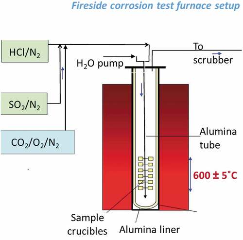
Table 2. Molar composition of the three different deposits used in the test.

Deposit	KCl	K2SO4		Na2SO4	CaSO4
	Concentration (mole %)
D1	30	20	20			30
D6	71	29
D8	67	33

Table 3. Composition of the simulated APR combustion gas environment.

Gas composition	N2	O2	CO2	SO2	HCl	H2O
Mol %	70.3	6.2	11.8	96.0 vol. ppm	53.0 vol. ppm	11.6

Prior to testing, samples were cleaned in an ultrasonic bath for 10 minutes with acetone, then iso-propanol (IPA). Dimensional measurements were carried out on the clean samples using a digital micrometre (resolution of 1 μm). The cleaned and measured samples were then weighed and put on a hot plate (temperature around 100°C), where deposit slurries were applied. Each slurry was applied with a flux of 100 μm/cm²/h on the convex face of the samples (deposit composition specified in Table 2); this was done to induce accelerated fireside corrosion damage [25–28]. The deposit was applied as a uniform layer on the samples’ surface, the amount of deposit was 20 mg per sample in every cycle.

In each cycle, samples were weighed prior to and after their deposits’ application. The weight data were used to track individual samples throughout the duration of the test and to check deposition fluxes. Individual samples were exposed for 200, 500 or 1000 hours for each combination of deposit and alloy type.

Post-exposure, samples were mounted in resin (with glass ballotini beads mixed into low shrinkage epoxy resin) to preserve any deposit/scale. The samples were then cross-sectioned, ground, and polished (down to to a 1 μm finish) with oil-based lubricant.

A statistical distribution of damage (change) was generated for all the samples via dimensional metrology [29–32]. All samples’ dimensions were measured prior to exposure to allow the correct calculation of dimensional changes post-exposure. Cross-sections of the exposed and polished cross-sectional samples were then measured with an image analyser and the position of the remaining metal and internal damage recorded around the sample. The image analyser then generated a set of x-y coordinates for the metal surfaces and any internal damage, which were compared to the ‘gas only’ damage recorded from a sample exposed to the same environment without any applied deposit. This procedure was necessary to isolate the damage caused by the deposit (rather than the gas). The data were when plotted and re-ordered to produce the final cumulative probability curves of the metal change and sound metal change (which is defined as metal change plus internal corrosion) associated with each material/deposit combination. Figure 3 gives a schematic diagram of the process. To take into account systematic errors inherent in the different measurement techniques (i.e. microscopy, micrometre), unexposed reference samples were used for calibration.

Figure 3. Schematic representation of the dimensional metrology process. The analysis consists of different steps 1) measuring the samples before exposure, 2) samples’ mounting in resin, 3) imaging of samples’ perimeters, 4) selecting of points at the metal surface and for internal damage, 5) comparing samples with pre-exposure measurements and reference samples, 6) subtracting the environmental effect by comparison to a sample exposed to the same environment without deposit, 7) plotting the resulting change in metal against location and 8) re-ordering the data based on cumulative probability [23,25].

The data presented as ‘metal change’ give an indication of the regression of the metal surface with respect to the original (i.e. pre-exposure) surfaces. These were the key output of this study and were produced in line with current standards for high temperature corrosion assessment [29–31]. Corrosion data analysis through statistical methods was proven to provide good basis for corrosion model development and validation [33,34]. Typical errors associated with this technique are in the range of about 3 to 5 μm [24].

Finally, scanning electron microscopy (SEM) was used to investigate the microstructure of scale layers that had formed on the alloys. Elemental analysis was also performed using energy dispersive x-ray spectroscopy (EDX).

Results and discussions

Dimensional metrology

For all alloy/deposit combinations, the distributions of the damage induced by fireside corrosion were collected after 200, 500 and 1000 hour exposure. These distributions are reported as metal change (or sound metal change) versus a cumulative probability (or standard deviation).

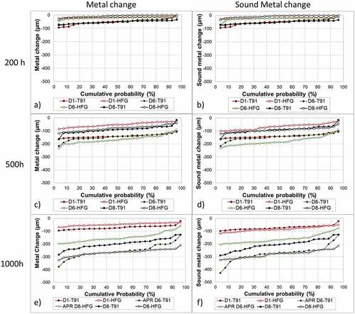
In Figure 4, the metal change distributions after 200, 500 and 1000 hour exposure are given (respectively Figure 4 a,c,e), as well as sound metal change distribution after 200, 500, 1000 hour exposure (Figure 4 b,d,f) respectively). The different curves represent the two alloys, T91 (full dots) and 347HFG (hollow dots), with the three different deposits D1 (red), D6 (green) and D8 (black). It can be seen from the metal change graphs, that the damage on the metal surface increases with an increase in the exposure time (Figure 4 a,c,e) for all the samples. This increase can be observed in the sound metal change graphs as well (Figure 4b,d,f).

Figure 4. Fireside distribution plot for metal change after a) 200 h; c) 500 h, e) 1000 h exposure; and sound metal change after b) 200 h, d) 500 h and f) 1000 h exposure, for both alloys and all three deposits.

Each metal or sound metal change value corresponds to a probability of finding a change equal or greater than the given value around the sample’s surface. In Figure 4, the distributions for all samples involved in the study are given. It can be seen that each alloy/deposit combination shows a different behaviour with respect to the others. In these graphs (Figure 4) the points on the extreme right side indicate a high probability (about 98% in this case) that the change in metal around the samples would be greater than the reported values. Other information can be extracted from the spread of the values. For example, the slope of the distribution can be related to the homogeneity of the corrosion damage around the surface of the samples.

Figure 5 report the median metal and sound metal changes for the two alloys and the two different deposits. It is worth nothing that samples without deposit were exposed at the same time for both alloys. Those samples showed a median metal change of −23.47 μm (T91) and −1.96 μm (347HFG). The median sound metal change recorded was equal to the median metal change for both alloys. Looking more closely at the deposits, different behaviours for each deposit can be observed. Samples coated with D1 (red curves; Figure 4) show a lower metal and sound metal change with respect to the other deposits for both alloys. The median metal changes recorded after 1000h exposure with deposit D1 for T91 and TP347HFG respectively were −74 μm and −45 μm, while the sound median changes were −75 μm and 86 μm. For the other deposits the median metal changes recorded were −260 μm and −170 μm for D6-T91 and D6-HFG respectively and −200 μm and −262 μm for D8-T91 and D8-HFG. This behaviour could be due to the different composition of deposit D1 as compared to D6 and D8 (see Table 2). The main difference between these three deposit is the availability of chlorides. In fact, D1 contains the lowest level of chlorides (KCl) (about 55% lower than D6 and D8).

Figure 5. Time distribution for the median metal and sound metal change. The bar chart shows the behaviour of the different alloys and different deposits. The error bars in the chart represent the maximum and minimum change of the different distributions.

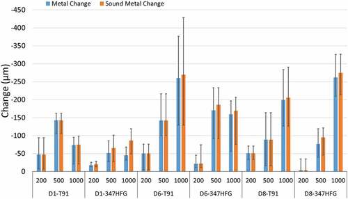
The other 2 deposits (D6 and D8) seem to have a different behaviour depending on the alloy (Figure 4). It appears that the deposit D6 has more impact over time on T91 steel leading to a higher metal and sound metal change (−260 μm and −270 μm, respectively), while D8 has more impact on 347HFG for both metal and sound metal change (−262 μm and −275 μm, respectively). The higher values for metal and sound metal change were recorded for the alloy 347HFG with deposit D8 and T91 with deposit D6, with both showing similar distribution (or amount of damage) after 1000 h exposure.

In Figure 6, SEM backscattered images for the different samples after 500 h are shown. From the pictures it can be seen how the scale/deposit layer on top of the T91 alloys (Figure 6 left hand side) is always detached from the alloy substrate, which is a clue of the fact that the metal is not able to form a protective oxide scale. At the same time, it can be seen that the scale/deposit layer on top of T91 is thicker than the one on top of 347HFG. Furthermore, no clear sign of internal damage can be observed inside the T91 samples. The roughness and small depletions of the metal surface of T91-D1 in Figure 6 and Figure 7, may suggest similar attacks for T91-D1 as seen for 347HFG, however, no grain boundary corrosion can be seen.

Figure 6. Backscattered images of the two different alloy and different deposits.

Figure 7. Backscattered images of T91-D1 and 347HFG-D1 on the left-hand side with respective EDX maps after 500 h exposure.

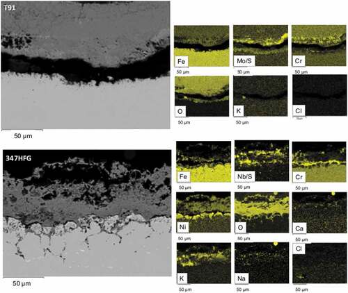
Figure 7 shows the EDX elemental analysis for both alloys covered with deposit D1. As it can be seen T91-D1 (Figure 7 top images) shows a porous layer of scale/deposit rich in Cr and Mo. It can also be noticed that the scale is detached from the alloy substrate. In the bottom images of Figure 7 the EDX analysis of 347HFG-D1 is reported. The EDX maps show the presence of S in the scale/deposit layer, which could be due to the presence of sulphates in the gas phase diffusing through the scale. The scale appears to be adherent to the substrate, and composed of Ni, Cr and Fe. Below the metal surface an area depleted in Cr and Fe can be seen. It also appears that the grains close to the metal surface show signs of intergranular corrosion attack and are surrounded by Cr-rich oxide. A similar behaviour was reported in literature [35,36] and named as ‘diffusion cell’ behaviour. This Cr-rich oxide would act as diffusion blocker, preventing the alloying elements from the bulk material, diffuse towards the surface of the metal, and create a protective oxide layer. Below the superficial grains, it can be seen how the damage is diffusing further into the alloy, but since the damage is not yet fully developed (e.g. grains are not surrounded by the Cr-rich oxide) no sign of Cr or Fe depletion was detected. Looking at the spatial distribution of Cl, it can be seen that the white precipitates on the left-hand side of the picture are composed by Cl. Those precipitates are found within grain boundaries. Furthermore, the diffusion of K inside the alloy was observed.

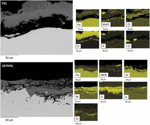
In Figure 8, T91 and TP347HFG samples exposed with deposit D6 are shown. In the top image, T91-D6 is shown, it can be seen that the scale/deposit layer is composed by Cr-Mo rich oxide, which is detached from the surface of the metal. For sample 347-D6 a similar behaviour of sample 347-D1 was observed (see Figure 7 and Figure 8). It can be seen that the scale on the metal surface is composed mainly by a Ni-rich oxide, and a Cr depleted region was found beneath the metal surface. Similar intergranular attack can also be observed, even though less pronounced respect to 347-D1 (Figure 7). Also, precipitates can be observed, which appears to be composed by Nb/S. Similar precipitates were found already in literature [37,38] e for Sanicro 25. Looking at the elemental maps, it can be seen a uniform spread of Cl across the metal surface (below Ni scale), this could be explained by the formation of a low melting point KCl-NiCl₂ eutectic mixture, with a Ni-Cl molten phase at temperature below 600°C [39].

Figure 8. Backscattered images of T91-D6 and 347HFG-D6 on the left-hand side with respective EDX maps after 500 h exposure.

In Figure 9 the samples with deposit D8 are shown. Sample T91-D8 is shown in the top left-hand side of the image, with elemental maps on the right-hand side. As it can be seen the scale/deposit layer in this case, looks denser, even though a detachment was observed in this case as well. The scale/deposit layer appears in this case composed of two different oxides. We can in fact observe a Fe-rich oxide in the top part of the layer, while a Cr-rich oxide can be seen close to the metal surface. It can be also noted the presence of K and S on top of the scale, which could indicate that part of the deposit is retained as K₂SO₄. Since the gaseous environment is rich in SO₂, this could have influenced grain boundary penetration.

Figure 9. Backscattered images of T91-D8 and 347HFG-D8 on the left-hand side with respective EDX maps after 500 h exposure.

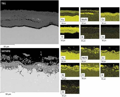
Looking at the sample 347-D8 (bottom image in Figure 9), it can be seen that features similar to the D1 and D6 are present. It can be seen an internal (intergranular) attack was suffered by the metal, and the presence of precipitates in the base alloy can be observed. Those precipitates appear to be formed by Nb/S, while an oxide layer surrounding the grains can be found, as for the previous samples. The presence of a Cr depleted region below the scale/deposit region can be observed.

In Figure 10 347-D6 after 1000 h exposure can be seen. A pit-like damage can be seen, which is filled with corrosion products, mainly Cl, O and Fe. This penetrative damage can be due to the high Cl vapour pressure, which could inhibit the ability of the scale of heal itself. Cl⁻ ions could also be lost from corrosion site, as illustrated in Figure 10. These ions could be released by ion exchange mechanism [20] and form HCl (gas, that could leave the corrosion site) in absence of KOH, via the mechanism described in equation 1.

(1) $C{l}^{-}+H_2{O}_{\left(g\right)}\overrightarrow{\leftarrow \phantom{{ }_{\text{vbox}to.5ex\text{vss}}}}HC{l}_{\left(g\right)}+O^{2-}\hspace{0.17em}$(1)

Figure 10. Backscattered image of 347HFG-D6 after 1000 h exposure, showing Cl attack mode.

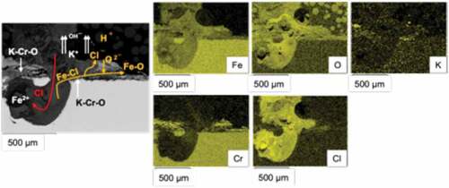
In absence of cations, there is a need to a sufficient provision of chlorides from deposit/gas, making the volume of chlorides the factor governing corrosion rates. The availability of chlorides would be influenced by the S/Cl ratio, which determine the eutectic melt fraction of the deposit [15].

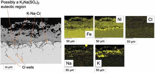
Deposit D1 could follow a different mechanism for the corrosion attack, due to the difference in deposit composition (see Table 2). In deposit D1 there is a simultaneous presence of Na and K, which could result in a lower melting temperature, respect to the K system only (as low as 310°C with 30% NaCl) [15,17,38]. In Figure 11, SEM data from 347HFG-D1 is reported after 500 h exposure. It can be observed that there is overlap in the Na, K and S maps (Figure 7 and Figure 11), which could suggest the formation of K₃Na(SO₄)₂ with low melting point [15]. This is in agreement with literature findings and could be formed through the reaction [15]:

(2) $4N{a}_{2}S{O}_{4_{\left(s\right)}}+4KC{l}_{\left(s\right)}\to 2K_{3}Na{(S{O}_4{)}_2}_{\left(l,s\right)}+6NaC{l}_{\left(s\right)}\hspace{0.17em}$(2)

Figure 11. Backscattered image of 347HFG-D1 after 500 h exposure showing K-Na possible location.

It can also be noted the penetration of the Cl beneath the metal surface (end tail of the intergranular attack in Figure 11), suggesting that the mixed scale could enhance the penetration of Cl inside the alloy. Similar behaviour was observed in literature by He et al [22], which suggested that a dual cation mix could result in more severe attack than single cation deposits, with cations playing a major role in the attack, facilitating the penetration of Cl through grain boundaries in 347HFG alloy. In addition to this, Ca and Na could have a role in the difference seen in corrosion. Those could increase the basicity of the salt mixture, which will alter the solubility of the different metal oxides [40].

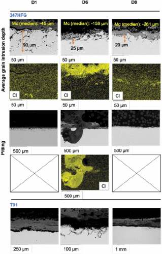
This was confirmed by SEM images (Figure 12) and penetration depth data (extrapolated from dimensional metrology data in Figure 4), where 347-D1 samples show higher extent of internal penetration respect to 347-D6 and 347-D8 samples. It is to be noted, even though penetration is lower for deposit D6 and D8 on 347HFG alloy, it shows the ability to form pit (especially D6). 347-D6 shows an evident pit which could be due to the high amount of Cl present in the deposit. D8 had also similar amount of Cl, but pits were not found, which could suggest that scale loss take place for this sample, leaving to a more evenly distributed front of attack [41]. Furthermore, deposit D8 and D6 showed the ability of starting on the surface of T91 after 500h of exposure, Figure 12. This was not observed for samples T91-D1, suggesting that the corrosion mechanism for the latter is different, and dependent on the presence of K, Na and Ca cations. These findings would explain the dimensional metrology data (see Figure 4) which showed higher damage for both D6 and D8 deposit, which contains a higher amount of Cl (see Table 2), that could lead to a higher molten fraction of the deposit.

Figure 12. Backscattered images and EDX maps for 347HFG with different deposits showing median penetration depth. Bottom figures represent T91 samples with different deposits after 500 h exposure.

In summary, the fireside corrosion rates and mechanisms under biomass simulated exposures partly depend on the hydroxide. Folkeson [21] discussed the role of KOH serving as intermediary between KCl and the diffusing Cl⁻ ions. In the case of this study, it is proposed that K₂CrO₄ could act as intermediary between KCl and Cl⁻, where scale decomposition products (OH in this case) support scale damage. It could so be argued that both Cl⁻ ion diffusion (which are likely to influence pitting formation) and alkali metal hydroxide transfers (which could influence scale damage) contribute to corrosive damage. The contemporary presence of Na and K it could be associated with the formation of lower melting point eutectics [16] (compared to system with only K as cation). In fact, low melting point K-Na-sulphate might form [16] and such compounds might make K less volatile and increase the molten deposit fraction.

Kung [42] proposed a different mechanism for the corrosion and especially the difference in the role of Cl and S in the fireside corrosion mechanisms. In his work, he supposed a different role for S, called ‘active sulfide-to-oxide corrosion mechanism’, in which S could combine with Fe, forming FeS at the interface between metal and scale. This will then form FeCl₂ which can diffuse through the scale and deposit as Fe₂O₃ on top of the scale. This behaviour could be somehow similar to what seen for T91-D6 (Figure 8), in which the presence of S has been detected at the interface between scale and the metal, and the contemporaneous presence of a Fe rich oxide in the outer scale.

Conclusions

In this paper, two stainless steel alloys (T91 and 347HFG) were exposed to a simulated combustion environment which could be generated from APR category fuels The samples were covered with three different deposits (D1, D6 and D8) designed to simulate vapour condensation from biomass post-combustion.

The samples were analysed by dimensional metrology and electron microscopy. The dimensional metrology data showed the increase of the damage with time for all exposure conditions. It also showed that the two alloys react differently to the different deposits, with T91 suffering a higher damage from deposit D8, while 347HFG showed higher damage for deposit D6.

The SEM/EDS data showed that different morphology for both the metal and scale/deposit. In fact, 347HFG showed internal damage attack, as intergranular corrosion, with a bigger penetration observed for deposit D1 samples. This was related to the lower chlorine level of deposit D1 in respect to D6 and D8. Deposit D1 is also composed by K, Na and Ca sulphate, which could have facilitated the Cl penetration through a multi-cations process. The pitting damage found 347-D6 was related to the higher Cl content in the deposit mixture, which is responsible of the surface lost. SEM/EDS data also confirm higher aggressivity of D6 and D8 deposits, that should be caused by the higher Cl content of the deposit, which could lead to a higher molten fraction.

T91 samples showed no signs of internal attack (for deposit D1), but it showed a more porous scale, that was always detached from the metals’ surface, signs of internal attack were reported for deposits D6 and D8, which contain higher Cl levels.

Disclosure statement

No potential conflict of interest was reported by the author(s).

Additional information

Funding

The author(s) are grateful for the financial support provided by BF2RA 28 towards this research, and also to Cranfield University for Industrial Partnership PhD scholarship support.

References

- Roadmap 2050:A practical guide to a prosperous. Brussels: Low-carbon Europe. European Climate Foundation; 2010.
- European Commission, State of play on the sustainability of solid and gaseous biomass used for electricity, heating and cooling in the EU. European Commission 2014. 10.1017/CBO9781107415324.004.
- A policy framework for climate and energy in the period from 2020 to 2030. European Commission 2014.
- Froggatt A, Hadfield A. Deconstructing the European energy union: governance and 2030 goals. UK Energy Research Centre; 2015.
- Camarsa G, Toland J, Hudson T, et al. LIFE and climate change mitigation. Luxembourg: European Union; 2015.
- Watson J, Gross R, Ketsopoulou I, et al. The impact of uncertainties on the UK’s medium-term climate change targets. Energy Policy. 2015;87:685–695.
- Sami M, Annamalai K, Wooldridge M. Co-firing of coal and biomass fuel blends. Prog Energy Combust Sci. 2001;27(2):171–214.
- Khodier AHM, Hussain T, Simms NJ, et al. Deposit formation and emissions from co-firing miscanthus with daw mill coal: pilot plant experiments. Fuel. 2012;101:53–61.
- Hussain T, Khodier AHM, Simms NJ. Co-combustion of cereal co-product (CCP) with a UK coal (Daw Mill): combustion gas composition and deposition. Fuel. 2013;112:572–583.
- Shao Y, Wang J, Preto F, et al. Ash deposition in biomass combustion or co-firing for power/heat generation. Energies. 2012;5(12):5171–5189.
- Wiltsee G, Consultants A Lessons learned from existing biomass power plants. n.d.
- Wilen C, Moilanen A. Kurkela espoo (Finland). energy production technologies]. Finland: E [VTT E. Biomass feedstock analyses; 1996.
- Michelsen HP, Frandsen F, Dam-Johansen K, et al. Deposition and high temperature corrosion in a 10 MW straw fired boiler. Fuel Process Technol. 1998;54(1–3):95–108.
- Mori S, Pidcock A, Sumner J, et al. Fireside corrosion of heat exchanger materials for advanced solid fuel fired power plants. Oxid Met. 2022;97(3–4):281–306.
- Mori S, Sumner J, Bouvet J, et al. Fireside and Steamside performance in biomass power plant. Materials at High Temperature. 2022;39(2):106–121.
- Niu Y, Zhu Y, Tan H, et al. A calculation method of biomass slagging rate based on crystallization theory. Asia-Pacific J Chem Eng. 2014;9(3):456–463.
- Simms NJ. 4 - Environmental degradation of boiler components. In: Oakey JE, editor. Power plant life management and performance improvement. Oxford: Woodhead Publishing; 2011. p. 145–179.
- Nielsen HP, Frandsen FJ, Dam-Johansen K, et al. The implications of chlorine-associated corrosion on the operation of biomass-fired boilers. Prog Energy Combust Sci. 2000;26(3):283–298.
- Karlsson S, Pettersson J, Johansson L-G, et al. Alkali induced high temperature corrosion of stainless steel: the influence of NaCl, KCl and CaCl2. Oxid Met. 2012;78(1–2):83–102.
- Pettersson J, Folkeson N, Johansson L-G, et al. The effects of KCl, K2SO4 and K2CO3 on the high temperature corrosion of a 304-Type austenitic stainless steel. Oxid Met. 2011;76(1–2):93–109.
- Folkeson N, Jonsson T, Halvarsson M, et al. The influence of small amounts of KCl(s) on the high temperature corrosion of a Fe-2.25Cr-1Mo steel at 400 and 500°C. Mater Corros. 2011;62(7):606–615.
- He J, Xiong W, Zhang W, et al. Study on the high-temperature corrosion behavior of superheater steels of biomass-fired boiler in molten alkali salts’ mixtures. Adv Mech Eng. 2016;8(11):1687814016678163.
- Global Steel & Alloys. ASTM A213/ASME SA213 T2, T11, T12, T22, T91, T92 chemical composition and mechanical properties 2021.
- Potter A, “Hot Corrosion in Industrial Gas Turbines,” PhD Thesis, Cranfield University, 2019
- Hussain T, Syed AU, Simms NJ. Fireside corrosion of superheater materials in coal/biomass co-fired advanced power plants. Oxid Met. 2013;80(5–6):529–540.
- Simms NJ, Kilgallon PJ, Oakey JE. Fireside issues in advanced power generation systems. Energy Mater. 2008;2(3):154–160.
- Syed AU, Simms NJ, Oakey JE. Fireside corrosion of superheaters: effects of air and oxy-firing of coal and biomass. Fuel. 2012;101:62–73.
- Hussain T, Syed AU, Simms NJ. Trends in fireside corrosion damage to superheaters in air and oxy-firing of coal/biomass. Fuel. 2013;113:787–797.
- Hussain T, Simms NJ, Nicholls JR, et al. Fireside corrosion degradation of HVOF thermal sprayed FeCrAl coating at 700-800°C. Surf Coat Technol. 2015;268:165–172.
- ISO - ISO 17224:2015 Corrosion of metals and alloys — test method for high temperature corrosion testing of metallic materials by application of a deposit of salt, ash, or other substances n.d. https://www.iso.org/standard/59451.html (2021 Oct 11).
- ISO - ISO 14802:2012 Corrosion of metals and alloys — guidelines for applying statistics to analysis of corrosion data n.d. https://www.iso.org/standard/53991.html (2021 Oct 11).
- ISO - ISO 26146:2012 Corrosion of metals and alloys — method for metallographic examination of samples after exposure to high-temperature corrosive environments n.d. https://www.iso.org/standard/54021.html (2021 Oct 11).
- Grabke HJ. Guidelines for Methods of Testing and Research in High Temperature Corrosion EFC 14. London: European Federation of Corrosion Publications; 1995.
- Stringer J, Wright IG. Current limitations of high-temperature alloys in practical applications. Oxid Met. 1995;44(1–2):265–308.
- Lu J, Yang Z, Li Y, et al. Fireside corrosion behaviors of super304h and HR3C in Coal Ash/Gas Environment with Different SO2Contents at 650 °C. J Mater Eng Perform. 2018;27(6):2855–2862.
- Evans HE, Taylor MP. Diffusion cells and chemical failure of MCrAlY bond coats in thermal-barrier coating systems. Oxid Met. 2001;55(1/2):17–34.
- Cruchley S, Evans H, Taylor M. An overview of the oxidation of Ni-based superalloys for turbine disc applications: surface condition, applied load and mechanical performance. Https. 2016;33:465–475.
- Rutkowski B, Gil A, Agüero A, et al. Chemical- and phase composition of sanicro 25 austenitic steel after oxidation in steam at 700 °C. Oxid Met. 2018;89(1–2):183–195.
- FactSage “FACT salt databases: database documentation.” https://www.crct.polymtl.ca/fact/documentation/. n.d.
- Rapp RA, Science C. 2002, 44(2), 209–221.
- Viklund P, Pettersson R. HCl-Induced high temperature corrosion of stainless steels in thermal cycling conditions and the effect of preoxidation. Oxid Met. 2011;76(1–2):111–126.
- Kung S,C. 2015, 71(4), 483–501.