A review of factors affecting the use of Electrical Potential Drop (EPD) for creep life monitoring

ABSTRACT

To help determine remaining lifetime of pressure vessels suffering creep, the authors have previously developed a method and presented promising results using a combination of AC and DC electrical potential drop (EPD) on-line monitoring, detecting both final cracking as well as incipient creep damage. The latter was tentatively ascribed to the development of cavitation damage, but recent modelling and separate off-line measurements have shown that cavitation is unlikely to provide enough of a change in electrical properties to explain all of the variations previously observed. Here we gather the results obtained to date, and review their likely relationships in an attempt to obtain a greater insight into the mechanisms at play. Whilst changes in both on-line and off-line EPD are largely in accord, the belief now is that the changes seen cannot be fully explained by cavitation development and that EPD is responding to other creep induced phenomena as well.

KEYWORDS:

• Potential drop
• EPD
• creep
• DCPD
• ACPD
• condition monitoring
• P91

Introduction & background

The use of the electrical potential drop (EPD) technique for monitoring creep damage in specimens and plant components at high temperature has been demonstrated by the authors in both the on-line laboratory and semi-industrial contexts [1] as well as off-line laboratory-based studies [2]. The latter have been aimed at trying to understand the EPD changes seen (for both alternating current (AC) and direct current (DC) regimes) during on-line monitoring. Both the on-line and off-line studies were conducted on welded specimens, where the EPD was monitored across heat affected zone (HAZ) locations thought to be particularly susceptible to type IV cracking (in P91/92 steel).

Normally employed for crack depth determination, EPD relies upon a measurement of a specimen’s electrical impedance. In the case of direct currents, this translates specifically into the electrical resistance, but with alternating currents, capacitive and inductive components join to generate a more complex response [3]. Any changes in the path that an electrical current takes, can alter impedance. In addition to cracks, other microstructural features are expected to alter impedance, such as the appearance of cavities.

On-line monitoring, by its very nature, prevents a deep study of those gradual changes in the underlying microstructure that may well affect the measured EPD, whilst studies on laboratory specimens often suffer from signal variations due to the multi-specimen nature, and loss of sensitivity, due to the interrupted testing. On-line monitoring measures an ‘average’ EPD response over a fixed location, whereas off-line measurements can be undertaken as area-scans, or ‘line-scans’, which gauge the changes in EPD across and along a specimen – and so give spatial information [2].

Results emanating from the on-line study showed a consistent and reproducible, if subtle, rise in DC EPD (DCPD) values, almost all of the way through the lifetime of the specimens (of the order of a 5% rise over a lifetime of ca.10,000 hrs) being tested (pressure vessels), and a commensurate drop in AC-EPD (ACPD). This was followed by rapid rises in both, just ahead of final fracture/rupture events. Off-line laboratory scans on creep specimens revealed changes in absolute ACPD that were consistent with those seen in the on-line tests. By measuring EPD line-scans traversing across the HAZ of welds (with the specimens themselves actually being cut out of much larger welds), it was possible to detect peaks in the EPD, particularly ACPD. Peak heights, when plotted as normalised values, against remaining lifetime, revealed a trend which appeared to provide a means of gauging consumed life through ACPD measurements.

One of the conclusions of the off-line EPD study [2], was that the changes seen in the EPD signals were highly likely to be due to cavitation damage – there being a reasonable link between independent measurements that showed a rise in the density and size of cavities – and the changes seen in the DCPD. Cavitation would theoretically have an effect on the effective resistivity of a conductor (or more precisely, its resistance) simply through an effect linked to geometric changes in the cross-section available for conduction. However, it is difficult to see how changes in magnetic permeability and other electromagnetic (EM) parameters (measured as part of an independent and parallel study [4]) could be ascribed to cavitation. Similarly, whilst a tentative link could be ascribed to the changes seen in the on-line DCPD results, explaining the reductions seen in on-line ACPD, in terms of cavitation appeared impossible. ACPD, and the linked EM measurements cited above [4], are more likely to be affected by the state of strain in a metal, and how this alters the shape and orientation of magnetic domains.

This paper details some of the results obtained in the off- and on-line studies and then attempts to relate them to some basic modelling that has since been conducted, to help shed light on the EPD responses observed. Given that the on-line changes seen were reproducible and the result of many separate experiments, this paper begins by making the assumption that DCPD (at least) was responding to cavitation. However, given the equation for the resistance of a conductor, a 5% rise in signal magnitude implies a 4.76% reduction in cross-sectional area – a feat for which cavitation volumes, as routinely reported for P91 is not expected to fulfil (see later). Thus, a simplistic view of cavities reducing the area available for conduction is insufficient to explain the observed changes. The development of cavities could, however, add to the path that electrons are required to take – and so raise the apparent resistivity, in essence lengthening the conductor in the cavitated zone via internal convolutions. Furthermore, the volume of actual metal (as distinct from the volume calculated from external dimensions) will not alter in a creep test, however there may well be lateral strain in the direction of the tensile load. This could alter, although subtly, the aspect ratio of the conducting “portions’ of the specimen and hence could, in theory, raise the resistance and hence the DCPD.

Overview of experimental work

For EPD, impedance is normally measured using a four-point arrangement of in-line electrical contacts, with the outer two connections delivering the excitation current, and the inner two allowing measurement of the potential drop required to drive the excitation current through the specimen [5]. Measurements are normally simplified by ensuring that the excitation current is known and remains constant during the measurement. A subtlety of ACPD over DCPD is the existence of the so-called ‘skin effect’, where the excitation current is found to travel close to the surface of the specimen, rather than uniformly throughout its cross-section (the latter being largely the case for DCPD). The depth that most of the current penetrates to (the skin depth) is a function of the frequency of the AC excitation, and this provides ACPD with an extra degree of freedom which can both add information or complicate interpretation (depending on one’s viewpoint!). The higher the frequency, the smaller the skin depth, and the more sensitive the technique to surface breaking defects.

EPD excels at providing a continuous electrical response that is proportional to crack dimensions and as such it is often the only crack monitoring technique that can be used in extreme testing contexts such as at high temperatures (e.g. thermomechanical testing of superalloys) [6], under corrosive atmospheres (e.g. H₂S induced cracking in the oil and gas industry, or stress corrosion cracking of stainless steels under high pressure high temperature aqueous conditions) [7], or even in high radiation environments (such as in-pile testing of materials in the nuclear industry). In such contexts, EPD is normally used in a continuous (on-line) sense to monitor for crack initiation and crack growth.

Aside from cracking, EPD can respond to a range of other effects that might be of interest including microstructural differences (such as within welds, or after case hardening), internal defects (e.g. porosity), residual stress measurements (ACPD is very sensitive to the level of elastic and plastic strain in ferrous materials). EPD may also offer an insight in other mechanism that would be expected to alter resistivity or impedance – such as hydrogen embrittlement (HE) or high temperature hydrogen attack (HTHA).

Many of the practical challenges associated with EPD relate to the engineering difficulties in the way in which electrical connections are made to specimens [3], and continuous monitoring in an industrial context poses additional difficulties associated with installation, such as access, the provision of power and external communication channels, as well as tight installation deadlines during plant outages.

For off-line non-destructive testing (NDT) applications, EPD equipment can be battery powered and then used for spot-checking of cracks in structures (particularly ACPD, given its better portability), with the 4-point connections being made by some kind of re-position-able or hand-held ‘probe’ head which usually houses sprung loaded pins able to penetrate surface oxides or contamination. However, resolutions reached (in terms of crack depth) are nothing like that achievable in an on-line context, mainly due to variabilities experienced in making reliable connections (and in locating the same measurement location after typical outage intervals have passed). Furthermore, hand-held spot checking is far more suited to ACPD than DCPD – simply because the excitation currents required when using DCPD are often far too high for the sprung contacts employed. Currents have to be in the 10ʹs of amps before a decent measurable DCPD can be obtained, depending on specimen sizes. Typical currents in ACPD studies are an order of magnitude less, but hand-held ACPD probes are very susceptible to registering changes in signal magnitude due to differences in approach angle and contact pressure.

These effects are linked to the existence of a variable error signal, known as ‘pick-up’ that superimposes upon the specimen-derived signal. Overall, such effects generally limit handheld EPD to a resolution of no better than 0.5 mm in crack depth measurements – significantly different from the 10 micron resolution that is normally achievable for typical cracks in a continuously monitored situation [6]. Using EPD for spot checking is therefore far from ideal, but has often been the methodology employed by plant operators and inspection companies, often leading to disappointment in the efficacy of EPD methods (especially for creep life determination).

On-line testing

In contrast to spot-checking, the application of EPD to long-term monitoring will suffer none of the issues described above; however, other than its common use in the laboratory as a means of measuring long-term fatigue crack growth, EPD seems to have been rarely used for on-line use, and this may have something to do with the practicalities of making robust connections in the field as well as interpreting the data generated. In 2015, the authors embarked on a long-term study of using EPD to detect and monitor creep damage in P91 and P92 steel pressure vessels undergoing laboratory testing. In this study, many of the practical issues associated with specimen connection and apparatus deployment were overcome. To date, data interpretation remains an on-going challenge although, as will be described here, the signs are that a path forward has been identified, with the main need being the acquisition of more data and installation experience to build up a database of EPD responses across different specimen geometries, environments and contexts.

Part of the advance made by the authors has been to combine the AC and DC variants into one monitoring system to effectively create an ‘AC/DC’-EPD set-up [1]. This has enabled the benefits and strengths of both variants to be captured in one on-line test, and has also revealed a synergistic effect which appears to greatly enhance an operator’s ability to determine (in this case) how close to end-of-life a monitored component is. We further describe this below when discussing the results of work already completed.

For the on-line work, the AC/DC set-up employed, required the interfacing of two commercial EPD instruments together, one providing ACPD capability and the other, DCPD, (Matelect Ltd, London). This was achieved by using a series of signal and current multiplexing (switching) units which also facilitated connection to multiple points on the test vessel. Several cylindrical pressure vessels were monitored in the three-year study. Figure 1 shows one of these, manufactured from P91 steel and containing two circumferential welds. The vessel was loaded axially and was also subjected to elevated temperature (ca. 700°C), and internal pressure (ca.100 bar). Failure was expected to initiate in the HAZ of the welds by Type IV cracking at around 10k hours, and it was these zones that were monitored by the EPD system. Scheduled outages occurred so that other off-line NDT characterisation methods could be employed, including ACPD in a hand-held mode.

Figure 1. Left – pressure vessel in open split-furnace, just after EPD connections have been completed. Right – routing and conversion of high temperature (HT) wiring to room temperature (RT) cabling.

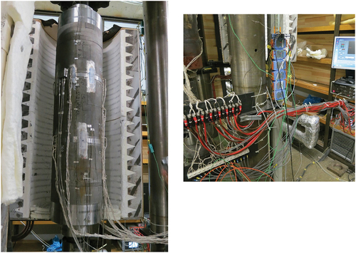
A significant feature of the on-line AC/DC system employed was the ability to use only one set of electrical connections for both EPD variants. This both simplified connections and reduced the number of wires and connection points to the test vessels, the only disadvantage being that the ACPD current carrying wires were, in effect, much thicker than they would normally be (given they also had to be capable of carrying the higher direct currents for DCPD).

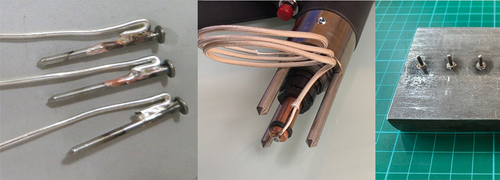
After much trial and error, a connection methodology which involved the use of stainless steel studs (ca. 20 mm long × 2 mm diameter) silver-soldered to pure silver wire, the whole being sheathed in silica braiding, was eventually employed. The studs were originally welded to the vessels using a conventional spot welder, and the wire silver-soldered in-situ. Specific engineering details on connection methodology can be found elsewhere [1] but the authors have since developed a system of welding which relies upon pre-wired and sheathed studs, and a specially developed stud welder, which uses a ‘gun’ type head (see Figure 2) that can deliver rapid and reliable connections at a very fast rate, allowing all the connections to be made in minutes rather than the hours that they originally took.

Figure 2. Left – pre-soldered stud connections ahead of installation, Mid – modified stud gun head. Right – rapidly welded stud array (minus wiring).

This process can now be enhanced even further by using 3D printed profiled ‘jigs’ which act as locators to ensure the arrays of connections are appropriately positioned, and the wiring suitably oriented and strain-relieved – creating a single ‘umbilical’ which is pre-manufactured at base, and can then be quickly installed in the industrial context. Normally, 4–8 connection locations are sufficient to adequately monitor one side of a weld, so a total of 16 ‘sites’ will cover the complete weld. This can generate a substantial umbilical containing nearly 100 sheathed wires.

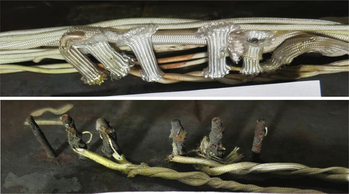
Silver wire of ca. 1.5 mm diameter was used for the current supply lines, and 0.5 mm for the signal lines. Silver was easy to handle in the field, thread through insulation, and solder in place. Its low resistivity meant that it was an ideal choice to be able to share AC and DC wiring, thus simplifying the umbilical up to the point where polymer sheathed, copper cabling was employed. Silver resisted the high temperature conditions well, and even after 10,000 hours of exposure, was always bright and free from oxidation, unlike the stainless studs which became heavily oxidised (see Figure 3).

Figure 3. Top – as made stud/wire connections ahead of creep test. Bottom – after 10k hour test duration – note unoxidised silver wire.

Typically, leads were 3 metres long from connection point on the vessel, to a nearby junction block (external to the furnace), and then to a set of signal and current multiplexers (and thence to the AC and DC instruments). To help eliminate interference or ‘pick-up’ in ACPD situations all wire pairs were twisted together, carefully done to avoid damaging the high temperature insulation.

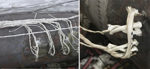
A total of 6 studs were positioned in-line across a weld to create a measurement ‘zone’ with the outer two studs delivering the requisite EPD excitation current, with the two inner pairs straddling each HAZ, and acting as the EPD measurement points (see Figure 4). Several ‘zones’ along any particular weld were thus covered.

Figure 4. Left – Stud connections after installation on horizontal vessel. Right – close up of a set of 6 studs, the outer two for the excitation current and two inner pairs for the signal from each HAZ.

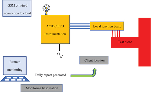
The EPD instrumentation was placed external to the furnace and blast zone (necessary because the vessels were pressurised), and placed under the control of bespoke software which could be accessed across the Internet, permitting the easy transfer of data for regular interpretation (as illustrated in Figure 5).

Figure 5. Schematic of a full AC/DC EPD system in a condition monitoring role. The local junction between RT (copper) and HT (silver) wiring is undertaken as soon as the HT wiring exits the hot zone.

Skin depth calculations for P91 steel, at the chosen excitation current frequencies suggested that even at the lowest operating frequency of 300 Hz, for the ACPD variant, the skin was significantly thinner than the specimen wall thickness (ca. 5 mm compared to 25 mm). This meant that the ACPD readings were only expected to reveal defects and/or microstructural variations that were close to the outer surface of the vessels. Past experience, however, suggested that crack development would initially be internal before travelling to either the outside surface or the inside (back-face) of a vessel. The lowest excitation frequency (300 Hz) was therefore expected to give the best chance of showing any internal or back-face defect. For reasons which are not entirely understood, subsequent work [2] indicated that a ‘sweet-spot’ in ACPD frequency of around 3 kHz existed – where sensitivity to incipient damage was maximised, so the parameters used in the original study may not have been optimal.

The AC excitation current was set to 2 amps for all measurements. In contrast, direct currents of ca. 50A are sometimes required for comparable signal magnitudes, but to minimise specimen heating and large voltage drops across the long cabling, 15A was the default excitation direct current chosen. A similar set-up was employed for other vessels in this study – one P92 vessel and a further P91 vessel, the only differences being that these latter vessels were mounted horizontally, and no external axial load applied.

On-line results and discussion

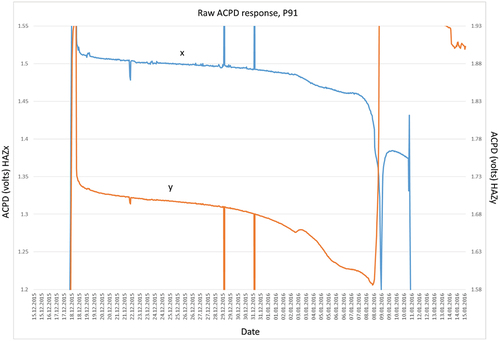
The study generated a mass of data over its 4-year period and much of this is described elsewhere [1], however the broad lessons for the use of EPD in a continuous monitoring role to detect incipient creep degradation, all the way to the final throes of a vessel’s life, can be drawn. Figure 6 shows a plot of extracted data for a typical DCPD response over a total period of just over 2.5 months from an adjacent pair of HAZ locations (designated ‘x’ and ‘y’) on the tested P92 vessel. There is clearly a large variation in signal magnitudes over time (this was mirrored by changes in monitored ACPD too).

Figure 6. DCPD over time (4 months) – initial rise to level due to heat up of furnace, with subsequent transients due to temperature control issues with furnace. The large swings far exceed that due to incipient damage by orders of magnitude.

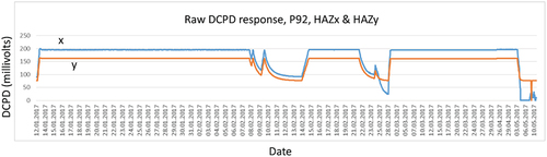
The fluctuations seen amount to several 10ʹs of % of full scale, which was eventually found to be substantially in excess of any fluctuation attributed to incipient damage (over months of exposure) – hence the earlier comment that changes due to cavitation and micro-crack development are likely to be very subtle. Once a crack had initiated and grown to be a substantial fraction of the specimen wall thickness, large changes in signal level might be expected, and indeed were observed, but clearly the fluctuations seen in Figure 6 recover in magnitude and level, and are definitely, therefore, not due to specimen cracking. Furthermore, such changes were often observed early on in the projected lifetime of the vessel, so could not be reasonably ascribed to cracking, in any sense. Most of these fluctuations were subsequently traced to changes in specimen temperature and/or failure of the apparatus applying internal pressure to the vessels.

To help deconvolute and deal with such signal changes, it was necessary to “normalise’ the data. In laboratory-based EPD, during elevated temperature testing, it is normal to employ a reference channel to normalise for temperature fluctuations. The reference location is ideally a ‘passive’ one, unlikely to be affected by the main ‘active’ phenomena being investigated, such as crack growth. A ratio of active/reference EPD is then calculated and this should be immune from changes in temperature. Normalisation by division was therefore employed in the pressure vessel study described here, but in the final analysis, normalisation was often found to not totally eliminate experimental fluctuations, most probably because the effect of temperature on the signals is likely to be non-linear or may involve signal components that are additive, and so cannot be completely eliminated through a simplistic mathematical division of active versus reference signals. This is especially expected to be the case when changes in pressure (hence strain) are factored in. ACPD is strongly affected by strain (in ferritic materials) [2] and not in a linear fashion. Notwithstanding this, a form of normalisation was employed in a post-processing sense. Thus, changes in signal magnitude in active areas were compared to those seen in passive/reference areas and if a similar trend was observed, the transient data could be offset or discounted totally – especially if the variations seen were small in duration (in relation to the overall testing duration). For this form of ‘normalisation’ to be applied effectively, other signals (such as temperature, pressure and/or strain) clearly need to also be monitored, compared and interpreted alongside the EPD data, if any certainty is to arise in practice. Other filtering methods can be employed to remove solitary transients which are clearly ‘rogue’ points.

Figure 7 illustrates what can be done using the approaches discussed. The data is now ‘noisier’ around a comparatively steady average, minus the large transient “noise’ seen before (as expected, given autoscaling has been employed to essentially raise signal gain).

Figure 7. Processed DCPD over time (2 months). Transients (any data 10% above or below running average) were removed, and data auto-scaled to reveal random signal noise. Slow but steady rise due to possible incipient damage then emerges.

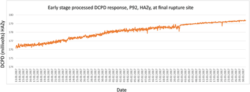
The y axis scale now reveals that noise in the EPD is at a level of 10ʹs of nanovolts – and hence is more likely to be a reflection of overall instrumental noise. Emerging from this noise can be seen a clear trend however – a gentle but steady rise in the EPD which is much more likely to be as a result of the development of creep damage. Given that this data set was obtained from a zone on the P92 vessel directly over where final rupture occurred, the authors had great confidence that they were detecting incipient damage.

Figure 8 reveals what was observed to happen to the EPD once a ‘real’ crack had initiated in one of the circumferential welds, in this case in one of the P91 vessels. The presence of the crack was confirmed after catastrophic failure of the vessel had occurred.

Figure 8. Raw DCPD over time (2 months) as final failure occurs – steady rise overtaken by exponential rise as crack propagates. Shielding effect on adjacent HAZ means complimentary DCPD drops.

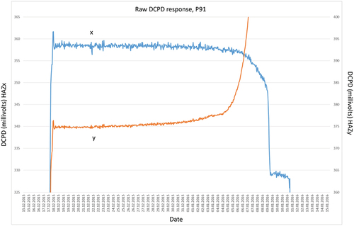
It should be noted that, as before, two signals were being monitored at this zone, namely one from either side of the weld, so that both HAZ were covered by AC and DC EPD measurements. The DC trends appear to work in opposition to each other with the one HAZ zone showing a clear exponential rise associated with a rapidly propagating defect, but the complimentary HAZ trace shows a gentle decline. The explanation for this is that both monitored zones are being fed the same excitation current and lie in line with each other (in terms of current flow) hence the growing defect will a) raise the DCPD (as conventionally expected) but b) divert the current flow away from the adjacent monitored HAZ such that it appears to show a reduction in measured DCPD. In other words, a developing defect shields the response from an adjacent monitored zone, so as one signal rises, the other falls.

It was clear that the change in the DCPD was very dramatic and highly definitive, when in the latter stages of failure (the last two days), but that nevertheless, a far subtler rise was seen at least two weeks ahead of failure. Such a gentle change would normally be ignored; however, when considered together with the drop seen in the adjacent HAZ’s response, a greater degree of certainty can be assumed that creep damage was developing. Additionally, when the complimentary ACPD response is considered alongside, a stronger pattern begins to develop – Figure 9 illustrates the corresponding ACPD traces, for the same locations on the P91 vessel, and here it can be seen that as the DC traces rise, the AC responses drop. Unlike for DCPD, this occurs on both HAZ positions and the drop continues until such time as the DC trace has begun its exponential rise, at which point the AC response follows suit, signifying rapid crack propagation.

Figure 9. Raw ACPD over time (2 months) at final failure – steady drop overtaken by exponential rise as crack propagates. Shielding effect on adjacent HAZ means complimentary ACPD drops. Transients not removed.

The explanation for the AC behaviour is not obvious and relies upon the knowledge that in ferritic materials, ACPD signals are sensitive to stress (strictly strain is the determining factor here) [8,9] as highlighted earlier. This is a result of the change in magnetic permeability that occurs when the grains containing magnetic domains are strained. As a result, in a ferritic material under a uniaxial stress, the ACPD measured axially has been observed to drop as the stress rises. In the monitored pressure vessel, the developing defect will be expected to raise the local stress to a point where the ACPD may indeed be affected by the stress concentration. Of course, the ACPD could also be responding to a rise in the general strain as a consequence of creep seen globally across the specimen. Strain gauges fitted to the pressure vessels did indeed register a gradual, if small rise, in global strains with time.

Overall then, given that the ‘true’ ACPD is normally only sensitive to surface breaking defects (as it relies upon the skin effect to generate a rise in path length as a defect grows) it is likely that the AC response over time will first drop (due to strain effects) before finally rising (presumably once the defect has become surface breaking).

When taken together, the drop in AC with the rise in DC, and the drop in DC on one HAZ, with a rise in the other, constitute a characteristic ‘signature’ which could greatly lengthen the warning period ahead of an impending failure when compared to the case of monitoring a single EPD response using one or other of the EPD variants. It is not unreasonable to suggest that alternative signatures could be identified, in other testing contexts.

The pattern of AC and DC EPD responses was repeated in all of the pressure vessel tests conducted to failure. Conservative estimates of the length of warning that the EPD monitoring system would have given test operators of a leakage, via a surface breaking defect, were in the region of two to three weeks for most specimens. This may well be sufficient notice for many plant operators.

The subtle (relatively), but steady, rise in DCPD seen in Figure 7 was actually present for some 2.5 months (ca. 1600 hours) before the test was terminated and the P92 test vessel examined using UT. No crack-like defects were detected, the EPD connections re-made, and the vessel was put back under test. The gentle rise in DCPD was observed to continue (at a similar, almost linear, gradient) until final cracking and failure occurred some 2 months later, whereupon a rapid rise in DCPD was observed (similar to that seen in the earlier P91 tests). The percentage change in DCPD amounted to less than a 1.5% rise over the initial 4.5 months, whereas the change in the last few hours of life amounted to over 100%. In this particular test, it was highly unlikely that a crack-like defect existed 4.5 months prior to failure, so lending weight to the notion that the subtle change in DCPD may well have been due to incipient damage.

Of the three on-line tests conducted to failure (2x P91 and 1x P92), all exhibited modest initial rises in DCPD readings close to the ultimate failure location.

Typically, over the total testing period of ca 10k hrs, the steady rise in DCPD, which we tentatively attribute to the build-up of cavitation and micro-cracking saw less than 5% rise in DCPD over the starting EPD values, but this was sufficient to signpost the build-up of creep-related damage.

Unfortunately, the testing timetable precluded termination of any test in the early stages of damage development and this particular study was more concerned with end-of-life determination, rather than remaining life prediction. These tests were therefore open to criticism that the changes in EPD seen could not be categorically ascribed to incipient creep damage – and in particular to the formation of creep cavitation. This prompted the follow-on study where controlled laboratory testing (on specimens taken from interrupted creep tests) was used to help determine the underlying phenomena responsible for the changes in AC and DCPD. The results of this follow-on study are fully reported elsewhere [2] but are summarised here in a direct comparison to the on-line testing.

Off-line testing

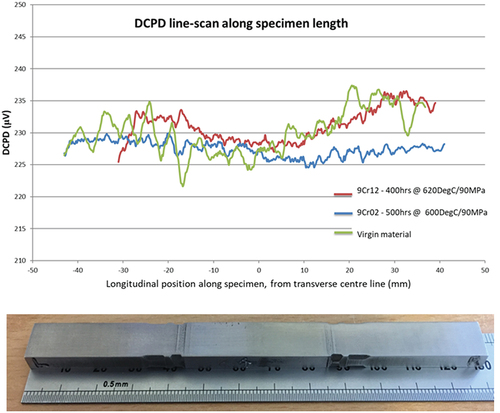
For this interrupted creep study, small test specimens (130 × 10 × 4.5 mm) were prepared (and creep tested) by research partners [4] and consisted of P91 material cut from a large (160 mm plate) pressure vessel multi-pass weldment (Figure 10), so as to contain 50% base metal and 50% weld metal, with the associated main heat affected zone (HAZ) located approximately mid-span along the specimen’s long axis and loading direction. Once again, failure was expected to initiate in the HAZ of the welds by Type IV cracking. It was these vulnerable zones that were monitored by the EPD system in the original on-line EPD study. Multiple specimens were machined and creep tested, under uniaxial load, at two temperatures (600°C and 620°C) for durations that corresponded to various (predicted) life fractions.

Figure 10. Top – DCPD line-scans along interrupted test specimens (bottom). Life fraction estimated to be less than 20% for these specimens over virgin material (also shown). No convincing trends can be detected.

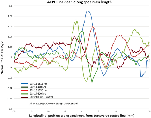
In addition to EPD, other characterisation techniques were also deployed by project partners – such as electromagnetic (EM) tests (e.g. magnetic Barkhausen noise (MBN) and measurements of magnetic permeability). For EPD, electrical connection to the specimen was made via sprung loaded pins but rather than being handheld, these were mounted in a computer-controlled X-Y table, so that surface scans of the specimens could be achieved. Computer software controlled the scanning procedure and, in this way, both area scans and line-scans could be made across the surface of a specimen. Results were processed in several ways – firstly to ascertain whether absolute changes in EPD were detectable, but also to judge the changes in EPD when scanning along a line down the tensile axis of the specimen. Some of these ‘line-scans’ are shown in Figures 10 and 11, given their relevance to the on-line data already discussed.

Figure 11. Top – ACPD line-scans along interrupted test specimens. Definite peaks are detectable, with central peak corresponding to location of HAZ. Further peaks (multiple passes?) can also be detected.

Off-line results and discussion

The results for DCPD scans were disappointing, and showed no statistically significant trend of absolute (averaged) DCPD with life fraction, although noticeable differences in DCPD level when traversing a HAZ were observed, indicating that DCPD is sensitive to microstructural effects. The reasons for this, and the contrast with the on-line study, are manifold but could simply be that the test specimens were not subjected to true life fractions.

What is also true is that the DCPD results were very much influenced by the location of the measurement on the specimen – with substantial edge effects seen in the area scans (unsurprising given the small size of the specimens). More details are given in the authors’ earlier publication [2] but these outcomes for DCPD further reinforce the notion, cited earlier, that the subtle changes in EPD are best detected via continuous monitoring, irrespective of the care and attention taken with interrupted ‘spot’ measurements.

In contrast, the off-line ACPD results showed a much more positive correlation with the previous on-line work, as well as far more dramatic changes in the signal level when traversing a specimen. Peaks in the absolute ACPD were detected at the HAZ (as opposed to the level changes seen in the DCPD results), and when the peak heights were plotted, a definite trend with life fraction was detected (see Figure 12).

Figure 12. Variation in ACPD peak height (main peak) with life fraction (estimated).

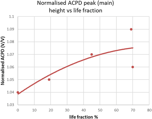
This trend was tentatively ascribed to a rise in the cavitation damage within the HAZ of the specimen (which appeared to correspond well with the location of the peaks in the line-scans). That said, what is significant about the ACPD results to the present discussion was the trend seen with the absolute (line averaged) ACPD taken across the whole specimen. This is shown in Figure 13, and revealed a definite drop over time, before recovering a little.

Figure 13. Variation in average ACPD (across main part of specimen) with life fraction (estimated).

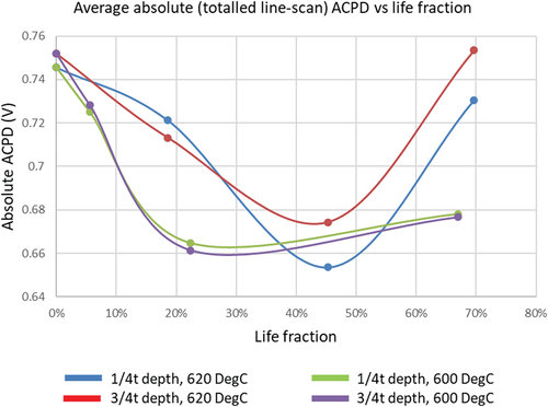
The response seen in Figure 13 accords with that seen in the on-line testing – namely a steady reduction in ACPD over time, until cracking becomes dominant and the PD begins to rise.

Measurements of magnetic permeability conducted by the partner researchers showed a similar trend in response – with the permeability dropping almost immediately with life fraction, and then reaching a minimum at about 50% of life. This again was encouraging in so far as the changes in ACPD are expected to be sensitive to changes in electromagnetic properties such as permeability, given they influence parameters such as the skin depth.

In conclusion, after considerable testing, in both on- and off-line contexts, it was clear that both ACPD and DCPD appeared sensitive to changes occurring in the pressure vessel steels experiencing creep. Ascribing these variations to actual creep-related phenomena remained speculative, given the nature of the testing and the inability to directly isolate any particular mechanism to check its effect on the EPD. Clearly, both AC and DCPD were very sensitive to end-of-life events such as catastrophic cracking, but the studies indicated far more subtle changes were detectable all the way through a specimen’s creep life. The major observations made from the on-line study were that ACPD appeared to gradually drop over time, across all monitored channels, whereas DCPD subtly rose over a similar period. This was partially supported by the off-line work which saw ACPD drop (in absolute terms) but also revealed spatial variations whose peak values rose over time. The latter could be ascribed to localised cavitation developing in the HAZ, leading to a rise in ACPD.

As mentioned earlier, the drop in ACPD is much more likely to be associated with the development of global strain (itself an indirect consequence of creep). Similarly, for DCPD, strain would be expected to have very little effect on signal magnitudes and the gradual rise in DCPD seen in the on-line measurements is much more likely to be a response to the development of cavitation. The fact that DCPD seems more sensitive to the effects of cavitation than ACPD is again explicable if one considers that DCPD is much more likely to respond to bulk changes than ACPD and that in any case, when considering ACPD, the effect of strain is probably far greater than the effect of cavitation – with the result that strain effects dominate the signal changes and the ACPD reduces.

Although all of this appears to ‘fit’ together in a plausible narrative, the fact remains that there is no sense of absolute magnitudes in any of this discussion – so the notion that strain dominates over cavitation in ACPD remains largely speculative. In an attempt to address this deficiency and actually ascribe some figures to known factors that could determine AC and DC responses, some basic modelling was conducted [10]. This work is reviewed in part below, given its likely relevance to the on and off-line studies that preceded it.

Modelling

For the purposes of modelling, a similar specimen geometry to that used in the laboratory off-line studies described above [2] was employed. This geometry, in turn, was as close as could reasonably be obtained to that in the on-line vessel tests also described above [1]. Although the overall specimen size, during on-line testing, was an order of magnitude larger than the off-line specimens, the way in which the currents are injected into the specimen (real or virtual), and the location and spacing of the electrical contacts, makes it unlikely that significant differences in current flow would occur between the various testing scenarios. It is the current flow and distribution that ultimately determines the fundamental potential drops.

The basic premise was to mesh a specimen with an array of cavities that could approximate to a damaged specimen – and to model the response with time (and cavity volume/number) once a series of virtual electrical connections had been made to it. This was conducted only for the case of DCPD, due to the greater simplicity of the DC case (modelling AC needs to consider other effects – for example the influence of strain on magnetic permeability) and because a clear target value of around 5% change in DCPD signal magnitude had been identified from the on-line vessel tests. If the model could generate such changes, then cavitation, by implication, could be the driver for these changes.

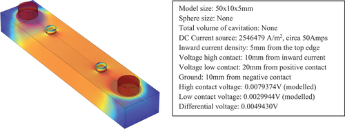
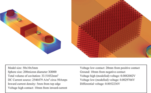
Meshing and modelling were carried out in COMSOL using the Joule heating subsection of the electromagnetic heating physics engine. A computer-aided design (CAD) model of the specimens and associated cavitation pores was created in Fusion360. The required 4-point electrical connection was then added, enabling the in-built ‘probe’ facility to interrogate a specific boundary and extract the resultant potential drop. The modelled system, was therefore close to ‘reality’, and any differences were regarded as unlikely to affect the validity of the results. Initially, a closer representation to the previously employed laboratory specimens was employed (Figure 14a and b) but far faster processing times (ca. 20 mins) were obtained by using a shorter specimen, with no significant alteration in the modelled current distribution and/or ‘measured’ voltage. Figure 15 shows the base-line reference specimen that was employed, and the parametric values chosen.

Figure 14. (a) LHS, meshed CAD model of test specimen, (b) RHS, modelled current distribution. Current is input/extracted via the two large posts on top surface. Voltages ‘read’ off on the inner two posts. DCPD is the differential value between inner contacts. Modelling parameters are given alongside.

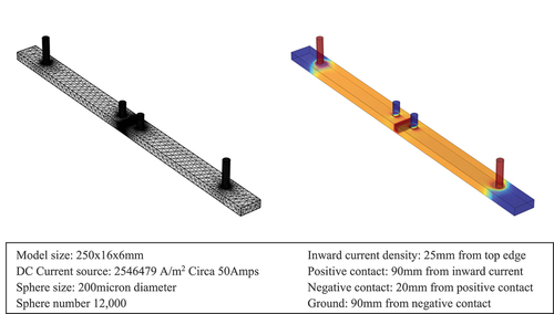
Figure 15. Simplified and shortened ‘reference’ specimen showing identical modelled current flow. Modelling parameters are given alongside.

It should be noted that the previous off-line tests [2] employed moving contacts (4 pin sprung-loaded probes) to deliver both the current and read the resultant voltage, whereas the model presented here has fixed contacts – so is actually much more applicable to the on-line tests [1] which used spot welded connections onto the pressure vessels under test. Once again, the difference was not deemed significant. The real purpose in the work was to ascertain whether cavitation is the likely driver for the DCPD signal changes previously observed.

The computational model defines the current injection at the top left of Figure 15, followed by a voltage (high) measurement point, a negative voltage (low) point, with the ground (zero) line being at the current exit point at the lower right-hand side. The DCPD signal is the calculated differential voltage between the high and low voltage measurement points.

In addition to the reference, nine other models were created, each with different numbers of cavities (ranging from 2,000 to 16,000). The cavities were modelled as spheres and were located in the central zone of the specimen (between the voltage ‘contacts’) in a volume of 5x5x10 mm (10 mm being the specimen width). All cavities were kept at 200 microns in diameter for the first batch of modelling.

Obtaining data on ‘real’ creep cavities is not always straightforward as both reported dimensions and cavity numbers vary in the literature. Renversade et al. [11] undertook an excellent study on cavitation in P91, and reported peak cavity sizes of around 2 microns in diameter for P91, and cavity densities of between 180k to over 700k per mm³. Again in P91, Han et al. [12] reported peak cavity sizes around double that of Renversade (although located in specimens with notch stress concentrations), and followed the coalescence of these, first into microcracks, and then macro defects. Even at 4 microns, these values proved too time consuming to model, and the decision was taken to raise cavity diameters to help make modelling feasible. Whilst this may have created an unrepresentative population of cavities (in P91 terms) it did allow the model to address the question of whether the practically observed changes in EPD could be ascribed to cavitation alone.

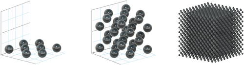
To mesh the cavities, a 1 × 1 mm 2D grid of 16 squares was created in Fusion360 in the X-Y plane. Eight spheres were inserted in this grid in a regular hexagonal array. In effect, every other square in the array was populated with a sphere (thus generating 8 cavities). This was expanded into 3D by adding layers in the Z direction, each rotated by 90 degrees with respect to the underlying layer. In total, 4 layers (each of 8 spheres) were generated and stacked together, as shown in Figure 16. This gave 32 spheres in total, in a 1 mm³ volume. This was then replicated to generate an array of spheres in a 5x5x10 mm³ volume followed by a Boolean subtraction to create a ‘cavitated’ volume of the same dimensions. Using this method, some 8000 cavities were evenly spaced in the 5x5x10 mm³ volume.

Figure 16. Cavity creation methodology, left to right, a single layer, a cube of layers, an array of cubes.

To generate alternative cavity populations, it was necessary to either add cavities or remove them from this basic array of 8000. By filling every space in the original 16 square grid with a sphere, it was possible to reach a cavity population of 16,000. Values of 6000, 4000, 2000 (and 10,000, 12,000, 14,000) cavities were generated by sequentially removing spheres from the 8000-cavity array (or the 16,000 array respectively) in an orderly fashion. Spheres were removed sequentially such that large gaps did not develop in the array (for example, avoiding two empty grid squares adjacent to each other).

It is acknowledged that the Boolean subtraction of cavities from the specimen is simplistic, and does not account for the fact that cavitation never removes material, it just reorganises it. The Boolean operation here employed actually removes conductive material from the model, so would be expected to generate a rise in DCPD that would exceed that for a constant volume model. Thankfully, this discrepancy would be most noticeable and significant at high cavity volumes, rather than at the much lower cavity volumes observed by Renversade et al. [11]. With this in mind, the assumption was made that the drop in material solid volume, at low cavity volumes could be neglected, with the change in DCPD being assumed entirely to be due to the alteration in current path and the additional constraint of the current being funnelled between cavities.

Modelling results and analysis

A typical modelled current distribution is shown in Figure 17a. As expected, the flow is largely uniform away from the immediate area of the current contacts, but appears concentrated in the zone of the cavity array. Figure 17b is a close up of this area. The banding that can be seen is again as expected, given the cavity layers are effectively separated from each other by thin un-cavitated zones – -which are more conductive and hence show up as a lighter colour. For a given thickness of cavitated material, and contact separation, the model might be expected to return a slightly lower DCPD than if the layers interpenetrated, simply because the current path would be more convoluted.

Figure 17. (a) LHS, modelled current flow in a cavitated specimen, for a cavity radius of 100 microns, and a cavity number of 8000, (B) RHS, close up of the cavitated area showing the banding in the current flow, characteristic of the model and the way in which the cavities are stacked.

The voltage outputs from each computed model are given in Table 1 together with the calculated values of total cavity volume (% porosity). Figure 18 plots the resultant DCPD against the % cavitation (porosity). The data is shown curve fitted to a 2nd order polynomial, with the extrapolation forced through the origin. Percentage porosity was chosen as the representative parameter to plot, so as to assist extrapolation of the resultant response to the more representative data on cavity size, as obtained from the literature.

Figure 18. Plot of calculated DCPD against % total cavitation (% porosity) for the constant cavity radius (variable cavity count) model. Equation fit given on plot.

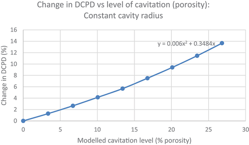
Table 1. Tabulated values of the modelled DCPD voltages and cavity volumes for a model with cavity size at 100 micron radius, but with variable cavity count.

Cavity radius (mm)	Single cavity vol (mm^3)	Total cavity vol (mm^3)	Calculated % change in DCPD	Calculated % porosity of test volume
0	0	0	0	0
0.2	0.03351	8.37758	1.298806	3.351,032
0.251984	0.067021	16.75516	2.700789	6.702064
0.28845	0.100531	25.13274	4.205948	10.0531
0.31748	0.134041	33.51032	5.83249	13.40413
0.341995	0.167552	41.88791	7.596601	16.75516
0.363424	0.201062	50.26547	9.522557	20.10619
0.382586	0.234572	58.64305	11.62654	23.45722
0.4	0.268083	67.02064	13.95913	26.80826

The data set shows that a 5% reduction in DCPD is easily demonstrated by the modelled array of cavities. By interpolation, a 5% change in DCPD would correspond to an approximate porosity of 12%, which equates to a little over 7000 cavities (of 200 micron diameter) in the 5x5x10 mm (250 mm³) zone. As discussed above, the modelled cavity sizes are some 2 orders of magnitude larger than the ones observed by Renversade et al. [11]. Their study presented a typical cavity count for their sampled volumes of around 5 × 10³ cavities, but for 2 micron diameter cavities, and sampled volumes were estimated to be cylinders of 0.6 mm diameter and 25 micron thickness, giving a cavity density (ρ_c) of approximately 7.08 × 10⁵ cavities per mm³. If these are assumed spherical, then each cavity has a total volume of 3.35 × 10⁻⁸ mm³, and the total percentage porosity in our modelled zone of 5x5x10 mm is given by:

$\mathrm{\%}\mathrm{p}\mathrm{o}\mathrm{r}\mathrm{o}\mathrm{s}\mathrm{i}\mathrm{t}\mathrm{y}=\frac{100\left(totalporevolume\right)}{\left(samplevolume\right)}=\frac{100\left({\rho }_c{V}_s{V}_c\right)}{V_s}=2.37\mathrm{\%}$

where V_c is the total volume of cavities, V_s is the cavitated-zone volume in the specimen and ρ_c is the cavity density (number per unit volume).

If this percentage porosity is substituted into the curve-fit data of Figure 18, an estimated percentage change in DCPD of 0.9% is generated. This is substantially lower than the 5% observed experimentally in the off-line tests.

Further analysis was performed on arrays of cavities where the cavity size was altered, but the cavity number maintained constant. This was done to test the interchangeability of cavity size with cavity number, and the results [10] gave an almost identical predicted change in DCPD of 0.89% Figure 19.

Figure 19. Modelled current flow in a cavitated specimen, for the constant cavity number model, (variable cavity size). 250 cavities shown, of 200 micron radius.

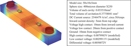
Whilst this current analysis relies upon an extrapolation to an effective pore size that is two orders of magnitude smaller than the smallest modelled, the close correspondence of both modelling approaches lends support that whatever parameter is altered, the modelled DCPD is primarily reliant on total percentage porosity (i.e. total cavity volume) rather than on the nuances of the morphology of the array of pores (which again seems a logical outcome). The implications for the two previous creep studies already described, and changes in observed DCPD therein are significant, for whichever of the two modelling approaches is taken – in particular, the assumption that the DCPD is determined by cavity volume alone has now been shown to be flawed.

The modelling approach taken here yields predicted DCPD changes that are only 20% of those seen in practice, if not smaller (given the large extrapolations that have been necessary in the modelled responses to attain ‘real’ cavity volumes), although hitting a similar order of magnitude via the modelling remains encouraging, even if some modification to the initial thesis and assumptions may be required.

A number of other factors could help to raise the observed changes in DCPD fivefold – for example, the possibility of cavities forming large local clusters, as creep proceeds – where the cavity volume might appear to grow predictably, but the cavity size and orientation might deliver a greater change in DCPD. Clearly, the cavities will eventually coalesce and form larger cavities – but these are unlikely to be spherical (as assumed by the modelling) with the possibility of longer aspect ratio cavities forming locally. Eventually, these cavities could take the form of embryonic cracks and thus the change in DCPD would be expected to take a different trajectory. Similarly, micro-cracking has been extensively identified as a stage in creep damage development in P91 weldments, (e.g. [11–13]) so the experimental data may in fact be initially responding to cavitation, but then become dominated by the development of micro-cracking or through cavity coalescence, to create macro defects.

Furthermore, it is likely that any coalesce of voids and the propagation of cracks be oriented perpendicular to the principal applied load, which in the work cited above [1,2] was also perpendicular to the line joining the current injection and voltage pick up points.

In this respect, such defects will be expected to further raise the measured DCPD, given the cracking directly interrupts the current flow by reducing the cross-sectional area for conduction. Similarly, any dilation in the specimen caused by localised strain in between cavities and cracks, will serve to further narrow and lengthen current paths, hence contributing to a rise in the DCPD. This latter effect, however, is expected to be orders of magnitude smaller than that due to a reduction in cross-sectional area for conduction (via cavity coalescence), simply from a geometric viewpoint, so should generate negligible changes to electrical resistance, and hence measured EPD.

Overall, it seems that all the likely factors that are contributing to the resistance of the specimen are working in harmony to raise the resistance (and hence the DC potential drop), so the five-fold discrepancy we see between the model and the experimental measurements may not be so irreconcilable after all, and certainly could be explained, either in part or in full, by a refinement of the model to include micro-cracking as a contributory factor.

Overall conclusions

The work presented here has attempted to synthesise a large body of experimental data on the EPD responses obtained from pressure vessel steels subjected to test conditions where creep damage is being generated. Both EPD variants have been found to respond to the final stages of creep damage, where large internal cracks develop and failure is imminent, so could be used for advanced notice of catastrophic failure. This has been adjudged to provide users with sufficient warning to be industrially ‘useful’ – but it is the more subtle longer-term changes in DC and ACPD that could offer a route to charting the incipient damage stages and hence help ascertain remaining lifetime or expended life. If such subtle changes could be reliably detected then EPD could offer a direct NDE method for remaining life determination, although clearly more work is required in order to transfer EPD to NDE application. On-line monitoring, however, was the mode of operation that was shown to be the most likely to achieve the necessary sensitivity to incipient damage, given the ‘noise’ expected in off-line measurements, so challenges remain if an off-line NDE methodology is sought.

In terms of ascribing to what the EPD changes observed are fundamentally due, several mechanisms come to mind, with the most obvious being cavitation development. As has been seen, however, computer modelling using a model that centred on the postulate of an array of spherical cavities, only revealed a modest rise in DCPD, and was not able to match the magnitudes of the experimentally determined rises. Although modelled DCPD values were typically a fifth of the experimentally observed values, this should not be viewed too negatively, for both the simplified nature of the model and the assumption that only cavitation is responsible for the changes seen, could be the reason for the discrepancies. The possibility remains, however, that other mechanisms are at play, which could further magnify up the measured DCPD – particularly those mechanisms that could be associated with embryonic or micro-crack formation, and the development of localised strains. Indeed, the gradual lowering of ACPD values seen experimentally (as the DCPD values rose) certainly suggests strain is strongly influential.

Overall then, although more work on the mechanistic aspects of the changes in EPD during creep damage development is recommended, EPD, per se, offers a route to damage detection and remaining lifetime prediction, with the combination of simultaneous AC and DC-EPD likely to provide the best outcomes.

Acknowledgments

The authors would like to thank Dr D Robertson of ETD Consulting, Leatherhead UK, for his help and support in undertaking the work described here and MPA Stuttgart for access to their facilities and universally helpful staff (especially Dr A Klenk and Dr A Hobt). Thanks also go to Dr Y Hasegawa of Sumitomo Metals, Japan, for access to the interrupted creep specimens, as well as Dr J Wilson and Prof. A Peyton, University of Manchester, UK, for sight of their EM results, and to Dr D Allen, of ETD Consulting, for life-fraction data and his helpful advice.

Disclosure statement

No potential conflict of interest was reported by the authors.

References

- Wojcik A, Waitt M, Santos AS. The use of the potential drop technique for creep damage monitoring and end of life warning for high temperature components. Mater High Temp. 2017;34(5–6):458–465.
- Wojcik A, Waitt M, Santos AS, et al. Electrical potential drop for monitoring creep damage in high temperature plant. Mater High Temp. 2021;38(5):330–341.
- A primer and guide to ACPD. Harefield (Uxbridge UK): Matelect Ltd; 2017.
- Wilson W, Peyton A, Allen D, et al., ‘The Development of an Electromagnetic (EM) sensor technique for creep damage detection and assessment’, Proceedings of the MIMA Conference, ETD Ltd, enquiries@etd- consulting.com;. 2020.
- Wojcik A. Potential drop techniques for crack characterisation. Mater World. 1995;3(8):379–381.
- Marchand NJ, Dorner W, Ilschner B. A novel procedure to study crack initiation and growth in thermal fatigue testing. ASTM STP. 1990;1060:237–259.
- Fanjiang M, Lu Z, Shoji T, et al. Stress corrosion cracking of uni-directionally cold worked 316NG stainless steel in simulated PWR primary water with various dissolved hydrogen concentrations. Corros Sci. 2011;53(8):2558–2565.
- Venkatsubramanian TV, Unvala BA. An AC potential drop system for monitoring crack length. J Phys E: Sci Instrum. 1985;17(9):765–771.
- Okumura N, Venkatasubramanian TV, Unvala BA, et al. Application of the AC potential drop technique to the determination of R curves of tough ferritic steels. Eng Fract Mech. 1981;14(3):617–625.
- Wojcik A, Santos AS, Waitt M, et al. Understanding signal changes when monitoring creep damage in high temperature plant using DCPD. Strength Fract Complex. 2022;15(1):47–57.
- Renversade L, Ruoff H, Maile K, et al. Microtomographic assessment of damage in P91 and E911 steels after long-term creep. Int J Mater Res. 2014;105(7):622–627.
- Han K, Ding H, Fan X, et al. Study of the creep cavitation behaviour of P91 steel under different stress states and its effect on high temperature creep properties. J Mater Res Technol. 2022;20:47–59.
- Venugopal S, Sasikala G, Kumar Y. Creep crack growth behaviour of a P91 steel weld. Procedia Eng. 2014;86:662–668.